Modelling reduced field dependence of $j_{\mathrm{c}}$ in YBCO films with nanorods

Abstract

Flux pinning is still the main limiting factor for the critical current of the high-temperature superconductors in high fields. In this paper we model the field dependence of the critical current in thin films with columnar defects aligned with the field. The characteristic shape of the critical current of the BaZrO₃ doped YBa₂Cu₃O_6+x thin films is reproduced and explained. The model is based on solving the Ginzburg- Landau equations with columnar defects present in the lattice. The size of the columnar defect is found to be of key importance in explaining the rounded shape of the critical current of the BaZrO₃ doped YBa₂Cu₃O_6+x thin films. It is also found that the size of the rod changes the long range order of the vortex lattice.

I Introduction

The critical current density, $j_{\mathrm{c}}$, of high-temperature superconductors in magnetic field is mainly limited by flux pinning Foltyn4 . Most of the envisioned applications, such as generators and fault current limiters, require the superconductors to have high critical current at magnetic fields of 3-5 T. In this range $j_{\mathrm{c}}$ is proportional to the fraction of vortices pinned in different pinning sites Pan3 . Each individual pinning site provides a pinning force, $f_{\mathrm{p}}$, which depends on the type of the pinning site. Typical pinning sites in YBa₂Cu₃O_6+x (YBCO) superconductors are dislocations, twins, antiphase boundaries, impurities and grain boundaries Foltyn4 . Out of these dislocations have been found most effective Dam2 , since they have the same shape as the vortices. Their effectiveness is limited by the small size of the core of the dislocation, 0.3 nm Svetchnikov1 , which is only a fraction of the vortex size in YBCO ($\xi=1.5$ nm at 0 K Blatter4 ). Twin planes pin vortices effectively if the current is parallel to the twin plane and thus the Lorentz force perpendicular to the plane, unfortunately if the current is perpendicular to the twin plane, the plane channels the vortices for easy movement, and therefore the $j_{\mathrm{c}}$ decreases Blatter4 ; Crabtree1 .

Doping the YBCO with e.g. BaZrO₃ (BZO) or BaSnO₃ (BSO) leads to formation of nonsuperconducting nanorods into the superconducting matrix MacManusDriscoll2 ; MacManusDriscoll8 ; Varanasi2 ; Varanasi5 . The nanorods act as very efficient pinning sites, since their diameter is around 5–10 nm Peurla3 ; Augieri5 and therefore around the same size as the vortex core. The nanorods are $c$-axis oriented and increase $j_{\mathrm{c}}$ at high fields especially when $B\parallel c$ Peurla3 ; Paturi15 .

The shape of the $j_{\mathrm{c}}$$(B)$ is most often described with the accommodation field, $B^{*}$, where the low field plateau ends and the exponent $\alpha$, which describes the decrease of $j_{\mathrm{c}}$ above $B^{*}$ with field $B^{-\alpha}$ Goyal4 ; Peurla3 ; Paturi17 ; Dam2 ; Klaassen2 . For typical undoped YBCO thin films the $B^{*}$$=$ 40–100 mT and $\alpha\approx 0.6$ Klaassen2 . In BZO-doped samples the $B^{*}$ increases up to 0.5 T and $\alpha$ decreases to 0.2 – 0.4 Peurla3 . The $\alpha$-value observed in undoped films is predicted by theories of strong sparse pinning sites Beek1 ; Nelson4 , but the lower value in the doped films has not been predicted, and finding a simple explanation for the lowered $\alpha$ value seems to be difficult due to the vortex-vortex interactions involved.

The problem in modelling flux pinning is that all the real samples contain many different kinds of pinning sites and the resulting $j_{\mathrm{c}}$$(B)$ consists of all the different interactions. It is relatively simple to calculate the pinning force of a single type of pinning site at low field Blatter4 , but even increasing the field, when vortex-vortex interactions come into play, makes the calculations in closed form impossible. Statistical approach has been used e.g. in refs. Pan3, ; Paturi16, ; Paturi18, ; Long4, ; Long5, and these models describe usually the shape of the experimental curves very well, but the understanding of e.g. the vortex paths inside the superconductors is limited.

The Ginzburg-Landau equations, although originally meant to be used close to the phase transition, describe superconductors well at lower temperatures too. Solving the minimum energy configuration for a certain set of parameters gives us the spatial variation of the order parameter $\psi$, which can be used to calculate the fraction of the pinned vortices as a function of e.g. the magnetic field or the density, shape and size of the pinning sites. The Ginzburg-Landau equations have been solved for small particles BarbaOrtega1 and with one or several pinning sites using $\delta T_{\mathrm{c}}$ pinning Machida1 and by restricting the order parameter Nakai1 . However, Crabtree et al. Crabtree1 present a large scale model with flux pinning that is similar to this work. Unfortunately, they do it for a relatively low $\kappa=4$ (low for modelling YBCO) and concentrate on the dynamics of the vortex trajectories instead of the critical current that is the focus of this work. We present a method for doing large scale computation of pinning in superconductors that are close to realistic size and calculate the field depedence of the critical current. In this paper we consider the case where magnetic field is parallel to the columnar defects. The results are directly compared to data from thin film YBCO samples.

II Computational model

II.1 Solving the Ginzburg-Landau equations

We chose to solve the static Ginzburg-Landau equations by finding a (local) minimum of the associated energy functional. For computational purposes, we write the energy in a dimensionless form. The only dimensional value is the overall energy scale, which does not affect the solutions and the dimensionless energy is

$$\begin{split}E=\int\text{d}^{3}{x}\bigl{(}\tfrac{1}{2}\lVert(\nabla+i{\vec{A}}){\psi}\rVert^{2}+\tfrac{1}{2}\lVert\operatorname{\nabla\times}{{\vec{A}}}\rVert^{2}\\ +\tfrac{1}{4}\kappa^{2}(\left\lvert\psi\right\rvert^{2}-1)^{2}\bigr{)},\end{split}$$ (1)

where $\kappa=\sqrt{\beta/(2\mu_{0}\hbar^{2}\gamma^{2}q^{2})}$ is the dimensionless Ginzburg-Landau parameter and $\gamma=1/(4m_{\mathrm{e}})$ and $q=2e$, the penetration depth is absorbed in the overall energy scale and therefore $\lambda=1$. Naturally, the coherence length is now simply $\xi=1/\kappa$. Equation (1) is then discretised as described in ref. Jaykka2, . In short, this discretization preserves the gauge invariance of the system and allows us to solve the equations without choosing and enforcing a gauge and the associated problems.

The solutions are then found using the TAO tao-user-ref and PETSc petsc-web-page ; petsc-user-ref ; petsc-efficient massively parallel numerical libraries. We account for the impurities in the physical system by using a bound constrained variant of the limited memory quasi-Newton algorithm (also called a variable metric algorithm) with BFGS Broyden1 ; Fletcher1 ; Goldfarb1 ; Shanno1 formula for Hessian approximations. This is provided by the TAO library. The impurities are then modelled by setting appropriate constraints for the Cooper pair density at the impurity locations. The gradients required by the algorithm are computed from the discretized energy in a straightforward manner.

The correctness and accuracy of the program was tested by solving the equations for a single Abrikosov vortex. At a $102^{2}$ lattice and lattice constant of $0.1\approx 0.07\xi$, the deviation from correct total energy is less than $0.02$ % with most of the deviation resulting from the small box: increasing the number of lattice points increases the accuracy. A smaller lattice constant does not increase the accuracy as much. Note that due to the rescaling, the lattice constant is in units of penetration depth $\lambda$. To be able to resolve the core of the vortex the lattice constant has to be smaller than $\xi$. This means that a lattice constant $h$ of approximately $0.1\xi$ gives very accurate results. Computer memory is a limiting factor in the computations. In practice, $h\approx 0.3\xi$ yields accurate enough results and requires $\approx 97$ % less computer memory.

At the $y$- and $z$-boundaries of the calculation $\psi$ is set to zero and the vector potential is kept fixed to simulate an external magnetic field. The $x$-boundary is periodic. Lattice sizes used in simulations were typically $500\times 520\times 50$ of which 10 pixels near the boundaries were used as vacuum ($\psi=0$, $\vec{A}$ is free). The vacuum between the sample and the calculation boundary allows for the magnetic field to bend around the sample which makes the external field of the simulation comparable to the actual field of the measurement of a thin film in a magnetometer.

As an example of a simulation result fig. 1 shows the absolute value of $\psi$ (fig. 1a) and the phase (fig. 1b) with $B=3$ T in a sample with dislocations. Using also the vector potential $\vec{A}$, the magnetic field $B_{z}=(\nabla\times\vec{A})_{z}$ (fig. 1c) and the current in the periodic direction $j_{x}=(\nabla\times\vec{B})_{x}/\mu_{0}$ (fig. 1d) were calculated. Note that also the shielding currents are visible. The calculation always yielded zero current in the vacuum, thus confirming the validity of the vacuum spacer layer.

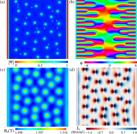
Figure 1: a) The absolute value of the calculated order parameter, $\left\lvert\psi\right\rvert$, shown on a plane sliced perpendicular to $c$-axis. b) The phase of the order parameter in the same calculation. c) The magnetic field density calculated from the vector potential in the same simulation and d) the current flowing in the periodic direction (up and down). Note that the scale is cut off short so that also the shielding current is visible.

II.2 Introducing pinning to the model and calculating $j_{\mathrm{c}}$

Flux pinning was modelled by locally restricting the maximum possible value of the real and imaginary parts of $\psi$ which then represents a pinning site. The chosen maximum value was 0.1 which corresponds to limiting the maximum value of $\left\lvert\psi\right\rvert$ between 0.1 and $\sqrt{2}/10$. The limit was not set to zero because that would have made the analysis of the result considerably more difficult. With this limit vortices can be defined to be the region of the calculation lattice where $\left\lvert\psi\right\rvert<0.1$.

The pinning sites had the same physical size and shape as is deduced from transmission electron microscopy (TEM) data: The BZO-nanorods were modelled as randomly distributed sample penetrating rods with a diameter of 5 nm Peurla3 ; Augieri5 . The dislocations were $c$-axis aligned sample penetrating rods with a diameter of 0.3 nm Svetchnikov1 , which were also randomly distributed in the sample.

The critical current was determined as the fraction of the vortex length trapped in the pinning site to the total length as in ref. Pan3, . Thus, we do not get the absolute values, but the field dependence of the $j_{\mathrm{c}}$ instead, which can be directly compared to the experimental data. The total length of vortices was calculated by following each vortex. If a point along the vortex is closer than $1.5\xi$ to a pinning site it was counted to the pinned section of the vortex. Finally, $j_{\mathrm{c}}$ is proportional to the fraction of the pinned sections to the total vortex length.

Modelling different pinning site types at the same time requires calculations over different length scales which is memory consuming. Dislocations are small in size and sparsely distributed which means large sample sizes are needed to contain more than a few dislocations. As a solution to this memory issue the coherence length and the pinscape were scaled up so that $\kappa=10$. Thus, we can use larger lattice constant allowing sparse dislocation densities. The change of $\kappa$ can be done without major changes to the physics Poole2 , since even at $\kappa=10$, we are at the limit of high-$\kappa$ and the magnetic field variation inside the superconductor is small. This was also verified by calculating two simulations with the same pinscape and resolution in units of $\xi$ but with different $\kappa$. Figure 2 shows the results of such calculations. It is easily seen that changing $\kappa$ does not have an appreciable effect on the results.

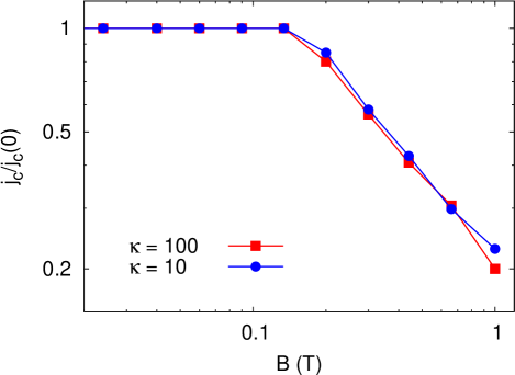
Figure 2: The same simulation calculated with $\kappa=10$ and $\kappa=100$. The change in $\kappa$ does not change the results.

III Results and discussion

The field dependence of $j_{\mathrm{c}}$ with BZO-nanorods as a pinscape was simulated for a 230 nm wide sample with thickness of 15 nm that is thick enough for the order parameter to reach 1 inside the sample and for all the relevant physics since here $\vec{B}$ is always perpendicular to the sample. The third direction was periodic with a period of 240 nm. There was also a 5 nm thick layer of vacuum around the sample. Both the rods and the magnetic field were parallel to $c$-axis. The magnetic field was varied from 4 T to 0 T with small steps. The result of the calculation with the previous field value was used as the initial condition for the calculation with the next field value. The density of the BZO-nanorods was set so that the matching fields were $B_{\phi}=1$ T (30 rods) and $B_{\phi}=2$ T (60 rods).

The $j_{\mathrm{c}}$ with dislocations as pinning sites was calculated with a similar calculation grid but its length was scaled by a factor of ten, due to the change in $\kappa$, to achieve the required low density of dislocations. The fine tuning of the dislocation density to match the experimental data was done after the simulation by scaling the length of the calculation lattice unit cell. The scaling does not alter the results because the pinning strength is determined by the ratio $r_{\mathrm{r}}/\xi$, and vortex-vortex interactions are affected by the ratio of the average pinning site separation to the penetration depth $\lambda$ which is also dimensionless. What the scaling does affect are the size of the sample and the value of the magnetic field. Thus, the sample size for the dislocation simulations was 530 nm (periodic) $\times$ 530 nm $\times$ 34 nm with dislocation densities corresponding to matching fields of 90 mT (12 rods), 180 mT (25 rods) and 360 mT (50 rods).

Figure 3 shows examples of simulation results at fields $B$ = 3 T and $B$ = 1.5 T with BZO-rods and dislocations as pinning sites. It can be seen that the strong pinning force of BZO-nanorods strongly disturbs the vortex lattice while pinning by dislocations results in a more regular vortex lattice. The modelled pinning sites can be seen in these images as larger circles (nanorods) and small dots (dislocations). It is easy to determine whether a pinning site is occupied when these images are combined with the information about the phase of $\psi$ and the pinscape coordinates.

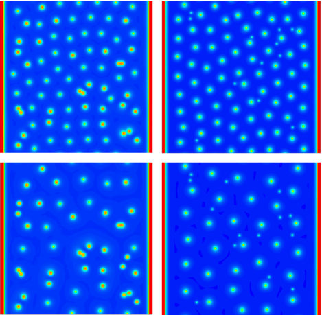
Figure 3: The absolute value of the calculated order parameter, $\left\lvert\psi\right\rvert$, shown on a plane sliced perpendicular to $c$-axis for nanorods (on the left) and dislocations (on the right) as pinning sites. The applied fields are 3 T (top) and 1.5 T (bottom). The scale of the images is the same as in fig. 1a.

The magnetic field scan from high field to low field was calculated using several random pinscapes with the same number of pinning sites. The results were taken as the averages of the critical currents derived from these simulations and the errors as the standard deviations of the simulation sets. In figure 4 we have overlayed the obtained $j_{\mathrm{c}}$$(B)$ for nanorods with 2.9 wt-% and 9 wt-% BZO-doped YBCO film data Peurla3 and the $j_{\mathrm{c}}$$(B)$ for dislocations with data from an undoped YBCO film. The $j_{\mathrm{c}}$ values have been scaled to 1 at zero field. The agreement with the experimental data is excellent and shows that the nanorods are so dominant in pinning that other pinning types can be neglected when the rods and the magnetic field are parallel. The $\alpha$ values for dislocation simulations range from 0.5 to 0.8 while for BZO-nanorods simulations gave $\alpha$ values of 0.26 and 0.41 for rod densities of 1 T and 2 T, respectively, which are quite typical values Klaassen2 ; Peurla3 ; Peurla1 ; Huhtinen12 ; Peurla4 ; Huhtinen16 ; Huhtinen20 . The $\alpha$ value of the measured pure YBCO thin film shown in fig. 4b is 0.59. Comparing the dislocation data to the experiments is more challenging because experimentally dislocation density is not so easy to adjust with the growth conditions while the density of the nanorods can be adjusted with the doping level. Further difficulties arise from the fact that dislocations do not dominate pinning so clearly as the large nanorods do. Thus, including other types of pinning sites (e.g. twins, oxygen vacancies) to the model is needed for more in depth analysis of the undoped films.

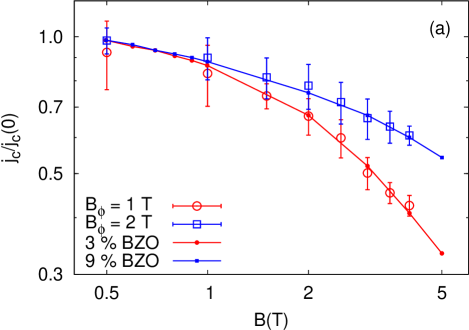
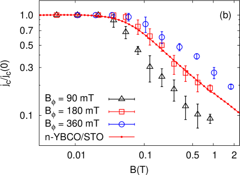
Figure 4: Calculated $j_{\mathrm{c}}$ (empty symbols) compared to experimental data (linespoints) when the simulation and sample contain a) nanorods and b) dislocations. The simulation point is an average over several different pinscapes and the errorbars are the standard deviations of those.

The nanorod data in fig. 4a shows a rounded shape of $j_{\mathrm{c}}$$(B)$ on log-log scale which is in contrast to the sharp bend between the different field regimes of the dislocation data in fig. 4b. Fitting $B^{-\alpha}$ to the rounded curves is difficult because the shape of the curve is not really correct unlike with dislocations. In this work $\alpha$ was determined from the part close to $B^{*}$ if the curve is rounded.

It would seem obvious to attribute the rounded shape of the BZO-nanorod data to the more dominant vortex-vortex interactions caused by the higher density of the defects. But the dislocations differ from nanorods also by size not only by density. Thus, we calculated $j_{\mathrm{c}}$ for a high density ($B_{\phi}=1.5$ T) pinscape with fixed defect locations but with variable rod radius $r_{\mathrm{r}}$ which is shown in fig. 5. From this it is clear that the typical rounded shape of the $j_{\mathrm{c}}$-curve of the BZO-nanorods requires not only a high density but also a large rod size. Having a high density of dislocations will not make the sample as good as one with a high density of BZO-nanorods.

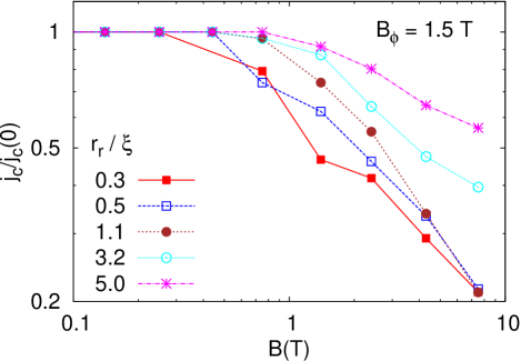
Figure 5: Calculated $j_{\mathrm{c}}$ with the same rod locations but different rod radii $r_{\mathrm{r}}$.

The results in fig. 5 were further analyzed by fitting $j_{\mathrm{c}}$$(B)=cB^{-\alpha}$ to the above $B^{*}$ portion of the datapoints. The obtained $\alpha$ values are shown in fig. 6. The values decrease with increasing rod diameter from 0.6 to 0.2 which is within the range of measured values for BZO and BSO nanorods schematically shown as ellipses in fig. 6. Naturally, the decrease of $\alpha$ comes from the deeper pinning potential of a larger rod which makes it possible for a vortex to sit in the potential well up to higher magnetic fields. The ellipses fit the simulation results even better if we take into account that in real samples nanorods are surrounded by additional defects which makes the rod effectively larger than the actual rod size measured with TEM and would thus move the ellipses to the right.

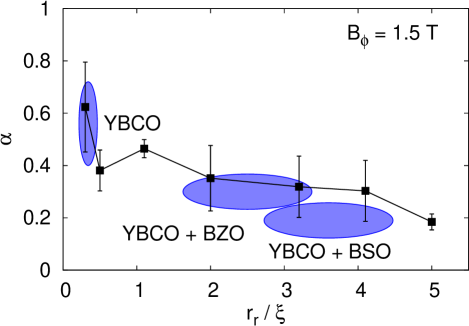
Figure 6: The $\alpha$ values from fits to curves in fig. 5. The error bars are the standard deviations of the fits. The range of experimental values measured for pure Peurla1 ; Huhtinen12 , BZO doped Peurla4 ; Huhtinen16 ; Huhtinen20 and BSO Varanasi2 ; Varanasi5 doped YBCO thin films is indicated with ellipses.

Furthermore, the accommodation field was calculated from the fit as $B^{*}=\mbox{}^{\alpha}\!\!\sqrt{c}$ i.e. the point where $cB^{-\alpha}$ intersects the line $j_{\mathrm{c}}$$(0)=1$. The accommodation fields relative to the matching field are shown in fig. 7. The accommodation fields level off to value $B^{*}/B_{\phi}=0.7$ starting from the rod size $r_{\mathrm{r}}/\xi=2$ which is the size where several vortices get pinned at a single rod. The $B^{*}/B_{\phi}=0.7$ is also seen in experiments Dam2 ; Klaassen2 . Assuming strong pinning by linear defects in low magnetic field the pinning potential per unit length $\epsilon_{\mathrm{r}}$ of the vortex is related to the accommodation field Blatter4 :

$$\frac{B^{*}}{B_{\phi}}\approx 4\frac{\epsilon_{\mathrm{r}}}{\epsilon_{0}},$$ (2)

where $\epsilon_{0}=\pi\hbar^{2}/(\mu_{0}q^{2}\lambda^{2})$ is the characteristic energy of the vortex per unit length. An analytical expression for the depth of the pinning potential of a cylindrical cavity has been derived in ref. Blatter4, as an upper limit within the London approximation:

$$4\frac{\epsilon_{\mathrm{r}}}{\epsilon_{0}}\approx 2\ln\left(1+\frac{r_{\mathrm{r}}^{2}}{2\xi}\right).$$ (3)

Using eqs. 2 and 3 the accommodation field can be roughly related to the pinning potential of the nanorods. But as can be seen from fig. 7 this relation between the accommodation field and the pinning potential seems to break down at large rod sizes where several vortices are pinned per rod.

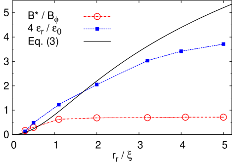
Figure 7: The depth of the pinning potential $4\epsilon_{\mathrm{r}}/\epsilon_{0}$ as a function of the rod radius $r_{\mathrm{r}}$ as calculated from the simulations (blue squares) and as given by eq. 3 (solid curve). The red circles show the ratio of the accommodation field $B^{*}$ to the matching field $B_{\phi}$ determined from the data shown in fig. 5.

The pinning potential of a nanorod was also determined by simulating a system consisting of a single vortex and a single nanorod. The depth of the potential was taken as the difference in the total energy between the state where the vortex is far away from the pinning site and where the vortex is pinned in the nanorod divided by the length of the rod. This was done for several rodsizes and the result is shown in fig. 7 where eq. 3 and the accommodation fields are also shown. Considering that there is no scaling or fitting involved the calculated potential depths are in general agreement with eq. 3.

Examples of more than one vortex pinned to a nanorod are shown in fig. 8. Up to four vortices get pinned to a large nanorod at high magnetic field. The vortices sit symmetrically at opposite sides of the rod. At rod size $r_{\mathrm{r}}/\xi=2$ the vortices are forced to be very close to each other but still there are two vortices in two of the rods. At rod size $r_{\mathrm{r}}/\xi=1$ there is only one vortex per rod. Ideally, there should be one vortex at each pinning site at the matching field. But the pinning sites are randomly distributed which makes them unevenly spaced. Thus, at small rod sizes the free vortices and the unoccupied pinning sites cancel out each other in the large scale giving the average of one vortex per pinning site. At large rod sizes this cancelling out happens by pinning several vortices at suitable sites while leaving some sites empty.

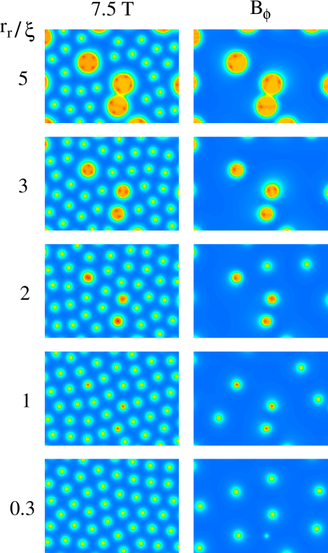
Figure 8: A closer look at 3 of the 55 nanorods in the simulations with varying rod size. The absolute value of the order parameter is shown with the color scale from 1 (blue) to 0 (red). The size of the images is 230 $\times$ 160 simulation grid points (130 nm $\times$ 90 nm). Simulation results in high magnetic field are on the left and at matching field (1.5 T) are on the right. The size of the nanorod decreases from top to bottom.

It is obvious from fig. 8 that the vortex lattice is more regular with the small nanorods. For a closer look into the short and long range order the radial distribution functions (fig. 9) of the vortex positions ($N\approx 250$) were calculated from the simulation results at 7.5 T. The vertical lines show the positions of the maxima for an ideal 2D-triangular lattice with the unit length of $a=(2\Phi_{0}/(\sqrt{3}B))^{1/2}$ where $\Phi_{0}$ is the flux quantum and $B=7.5$ T. There are 4 broad peaks visible at the rod size 0.3 which roughly overlap the positions of the ideal case. The 4th peak corresponding the 6th and 7th nearest neighbour (NN) is already very weak. There is no long range order past the 7th NN at any rod size. At the rod size $r_{\mathrm{r}}/\xi=3$ and larger only the first NN peak is visible. Thus, the triangular vortex lattice continues over the small rods with some disturbance while the large rods completely break down the long range order. Since the area of the first peak is constant the coordination number is the same for all rod sizes. The pinning of several vortices to the same pinning site has been experimentally observed e.g. in ref. Bezryadin2, where the irregularity of the vortex lattice near the pinning sites is clearly visible too.

Figure 9: The radial distribution functions of the vortex core positions for the different nanorod sizes. The vertical lines mark the positions of the nearest neighbours for an ideal 2D-triangular vortex lattice at 7.5 T.

From the experimental point of view the results presented here further emphasize that one should not only focus on optimizing the density of the pinning sites but the size of the defects needs to be carefully considered too. Naturally, if the magnetic field in the application is not homogenous one needs to consider the splay of the nanorods too. In large scale production, where in situ deposition is almost the only option, the size of the defect is fixed by the chemical properties of the dopant MacManusDriscoll8 . Thus, one has to try different dopant materials to find those that produce large enough columnar defects. With large defects the optimal density is a compromise between the superconducting volume and pinning. However, at large defect sizes, where several vortices get pinned to each defect, it is clear that any density (in terms of matching field) of the defects above the operating field of the application is not optimal since some of the defects will be left empty. On the other hand, if there are two vortices per rod, a density of half the operating field is too low because some of the rods will only pin one vortex due to e.g. the variation in the rod positions. With naive arguments one can say that having one vortex per rod is better than two since with two vortices the rod diameter has to be roughly twice as large which increases the volume of the rods by a factor of 4. But in reality there is a lot of different strains and relaxations involved when the distance between the rods is changed which could compensate for the loss of the superconducting volume by increasing $T_{\mathrm{c}}$ and $j_{\mathrm{c}}$(0).

IV Conclusions

In this paper we have shown that it is possible to model flux pinning numerically with the Ginzburg-Landau equations. The model fully includes vortex-vortex interactions which is very important for modelling flux pinning. Doing this allows us to see the vortex paths inside the sample and to calculate the field dependence of $j_{\mathrm{c}}$ for a pre-determined pinning site configurations. The results are in excellent agreement with the experiments.

The main result was that the reason behind the characteristic round shape of the $j_{\mathrm{c}}$ and the lowered $\alpha$ value of the BZO-doped YBCO films is not only the high density but also the large size of the pinning sites. The density of the pinning sites acts through the vortex-vortex interactions while the rod size (i) changes the depth of the pinning potential, (ii) changes the number of the pinned vortices per rod, (iii) and supresses the long range order of the vortex lattice at larger sizes.

The current model can also be used to simulate the angular depedency of $j_{\mathrm{c}}$ which will be our next objective. Adding time and current to the model by using time-dependent Ginzburg-Landau will allow transport measurement simulations.

- (1) S. R. Foltyn, L. Civale, J. L. MacManus-Driscoll, Q. X. Jia, B. Maiorov, H. Wang, and M. Maley, Nat. Mater. 6, 631 (2007)
- (2) V. Pan, Y. Cherpak, V. Komashko, S. Pozigun, C. Tretiatchenko, A. Semenov, E. Pashitskii, and A. V. Pan, Phys. Rev. B 73, 054508 (2006)
- (3) B. Dam, J. M. Huijbregtse, F. C. Klaassen, R. C. F. van der Geest, G. Doornbos, J. H. Rector, A. M. Testa, S. Freisem, J. C. Martinez, B. Stuble-Pumpin, and R. Griessen, Nature 399, 439 (1999)
- (4) V. Svetchnikov, V. Pan, C. Træholt, and H. Zandbergen, IEEE T. Appl. Supercond. 7, 1396 (1997)
- (5) G. Blatter, M. Feigel’man, V. Geshkenbein, A. Larkin, and V. Vinokur, Rev. Mod. Phys. 66, 1125 (1994)
- (6) G. W. Crabtree, D. O. Gunter, H. G. Kaper, A. E. Koshelev, G. K. Leaf, and V. M. Vinokur, Phys. Rev. B 61, 1446 (2000)
- (7) J. L. MacManus-Driscoll, S. R. Foltyn, Q. X. Jia, H. Wang, A. Serquis, L. Civale, B. Maiorov, M. E. Hawley, M. P. Maley, and D. E. Peterson, Nat. Mater. 3, 439 (2004)
- (8) J. L. MacManus-Driscoll, S. A. Harrington, J. H. Durrell, G. Ercolano, H. Wang, J. H. Lee, C. F. Tsai, B. Maiorov, A. Kursumovic, and S. C. Wimbush, Supercond. Sci. Technol. 23, 034009 (2010)
- (9) C. V. Varanasi, P. N. Barnes, J. Burke, L. Brunke, I. Maartense, T. J. Haugan, E. A. Stinzianni, K. A. Dunn, and P. Haldar, Supercond. Sci. Technol. 19, L37 (2006)
- (10) C. V. Varanasi, J. Burke, L. Brunke, H. Wang, M. Sumption, and P. N. Barnes, J. Appl. Phys. 102, 063909 (2007)
- (11) M. Peurla, P. Paturi, Y. P. Stepanov, H. Huhtinen, Y. Y. Tse, A. C. Bódi, J. Raittila, and R. Laiho, Supercond. Sci. Technol. 19, 767 (2006)
- (12) A. Augieri, G. Celentano, V. Galluzzi, A. Mancini, A. Rufoloni, A. Vannozzi, A. A. Armenio, T. Petrisor, L. Ciontea, S. Rubanov, E. Silva, and N. Pompeo, J. Appl. Phys. 108, 063906 (2010)
- (13) P. Paturi, M. Irjala, and H. Huhtinen, J. Appl. Phys. 103, 123907 (2008)
- (14) A. Goyal, S. Kang, K. J. Leonard, P. M. Martin, A. A. Gapud, M. Varela, M. Paranthaman, A. O. Ijadoula, E. D. Specht, J. R. Thompson, D. K. Christen, S. J. Pennycook, and F. A. List, Supercond. Sci. Technol. 18, 1533 (2005)
- (15) P. Paturi, M. Irjala, A. B. Abrahamsen, and H. Huhtinen, IEEE T. Appl. Supercond. 19, 3431 (2009)
- (16) F. C. Klaassen, G. Doornbos, J. M. Huijbregtse, R. C. F. van der Geest, B. Dam, and R. Griessen, Phys. Rev. B 64, 184523 (2001)
- (17) C. J. van der Beek, M. Konczykowski, A. Abal’oshev, I. Abal’osheva, P. Gierlowski, S. J. Lewandowski, M. V. Indenbom, and S. Barbanera, Phys. Rev. B 66, 24523 (2002)
- (18) D. R. Nelson and V. M. Vinokur, Phys. Rev. B 48, 13060 (1993)
- (19) P. Paturi, M. Irjala, H. Huhtinen, and A. B. Abrahamsen, J. Appl. Phys. 105, 023904 (2009)
- (20) P. Paturi, Supercond. Sci. Technol. 23, 025030 (2010)
- (21) N. J. Long, N. M. Strickland, and E. F. Talantsev, IEEE T. Appl. Supercond. 17, 3684 (2007)
- (22) N. J. Long, Supercond. Sci. Technol. 21, 025007 (2008)
- (23) J. Barba-Ortega, E. Sardella, and J. A. Aguiar, Supercond. Sci. Technol. 24, 015001 (2011)
- (24) M. Machida and H. Kaburaki, Phys. Rev. Lett. 75, 3178 (1995)
- (25) N. Nakai, N. Hayashi, and M. Machida, J. Phys. Chem. Solids 69, 3301 (2008)
- (26) J. Jäykkä, Phys. Rev. D79, 065006 (2009)
- (27) S. Benson, L. C. McInnes, J. Moré, T. Munson, and J. Sarich, TAO User Manual (Revision 1.9), Tech. Rep. ANL/MCS-TM-242 (Mathematics and Computer Science Division, Argonne National Laboratory, 2007) http://www.mcs.anl.gov/tao
- (28) S. Balay, K. Buschelman, W. D. Gropp, D. Kaushik, M. G. Knepley, L. C. McInnes, B. F. Smith, and H. Zhang, “PETSc Web page,” (2009), http://www.mcs.anl.gov/petsc
- (29) S. Balay, K. Buschelman, V. Eijkhout, W. D. Gropp, D. Kaushik, M. G. Knepley, L. C. McInnes, B. F. Smith, and H. Zhang, PETSc Users Manual, Tech. Rep. ANL-95/11 - Revision 3.0.0 (Argonne National Laboratory, 2008)
- (30) S. Balay, W. D. Gropp, L. C. McInnes, and B. F. Smith, in Modern Software Tools in Scientific Computing, edited by E. Arge, A. M. Bruaset, and H. P. Langtangen (Birkhäuser Press, Boston, 1997) pp. 163–202
- (31) C. G. Broyden, J. Inst. Math. Appl. 6, 76 (1970)
- (32) R. Fletcher, Comput. J. 13, 317 (1970)
- (33) D. Goldfarb, Math. Comput. 24, 23 (1970)
- (34) D. F. Shanno, Math. Comput. 24, 647 (1970)
- (35) C. P. Poole, H. Farach, R. Creswick, and R. Prozorov, Superconductivity, Second Edition (Academic Press, 2007) pp. 347
- (36) M. Peurla, H. Huhtinen, and P. Paturi, Supercond. Sci. Technol. 18, 628 (2005)
- (37) H. Huhtinen, M. Peurla, M. A. Shakhov, Y. P. Stepanov, P. Paturi, J. Raittila, R. Palai, and R. Laiho, IEEE T. Appl. Supercond. 17, 3620 (2007)
- (38) M. Peurla, H. Huhtinen, Y. Y. Tse, J. Raittila, and P. Paturi, IEEE T. Appl. Supercond. 17, 3608 (2007)
- (39) H. Huhtinen, K. Schlesier, and P. Paturi, Supercond. Sci. Technol. 22, 075019 (2009)
- (40) H. Huhtinen, M. Irjala, P. Paturi, and M. Falter, IEEE T. Appl. Supercond. 21, 2753 (2011)
- (41) A. Bezryadin, Y. N. Ovchinnikov, and B. Pannetier, Phys. Rev. B 53, 8553 (1996)