On Quantification of Anchor Placement

Abstract

This paper attempts to answer a question: for a given traversal area, how to quantify the geometric impact of anchor placement on localization performance. We present a theoretical framework for quantifying the anchor placement impact. An experimental study, as well as the field test using a UWB ranging technology, is presented. These experimental results validate the theoretical analysis. As a byproduct, we propose a two-phase localization method (TPLM) and show that TPLM outperforms the least-square method in localization accuracy by a huge margin. TPLM performs much faster than the gradient descent method and slightly better than the gradient descent method in localization accuracy. Our field test suggests that TPLM is more robust against noise than the least-square and gradient descent methods.

1 Introduction

Accurate localization is essential for a wide range of applications such as mobile ad hoc networking, cognitive radio and robotics. The localization problem has many variants that reflect the diversity of operational environments. In open areas, GPS has been considered to be the localization choice. Despite its ubiquity and popularity, GPS has its Achilles’ heel that limits its application scope under certain circumstances: GPS typically does not work in indoor environments, and the power consumption of GPS receiver is a major hindrance that precludes GPS applications in resource-constrained sensor networks.

To circumvent the limitations of GPS, acoustic/radio-strength and Ultra-wideband (UWB) ranging technologies have been proposed [10, 22, 11]. Measurement technologies include (a) RSS-based (received-signal-strength), (b) TOA-based (time-of-arrival), and (c) AoA-based (angle-of-arrival).

RSS-based (received-signal-strength) technologies are most popular mainly due to the ubiquity of WiFi and cellular networks. The basic idea is to translate RSS into distance estimates. The performance of RSS-based measurements are environmentally dependent, due to shadowing and multipath effects [22, 25, 3]. TOA-based technologies such as UWB and GPS measures the propagation-induced time delay between a transmitter and a receiver. The hallmark of TOA-based technologies is the receiver’s ability to accurately deduce the arrival time of the line-of-sight (LOS) signals. TOA-based approaches excel RSS-based ones in both the ranging accuracy and reliability. In particular, UWB-based ranging technologies appear to be promising for indoor positioning as UWB signal can penetrate most building materials [10, 22, 11]. AoA-based technologies measure angles of the target node perceived by anchors by means of an antenna array using either RRS or TOA measurement [22, 11, 2]. Thus AoA-based approaches are viewed as a variant of RRS or TOA technologies.

Rapid advances in IC fabrication and RF technologies make possible the deployment of large scale power-efficient sensor networks. The network localization problem arises from such needs [26, 6]. The goal is to locate all nodes in the network in which only a small number of anchors know their precise positions initially. A sensor node (with initially unknown position) measures its distances to three anchors, and then determines its position. Once the position of a node is determined, then the node becomes a new anchor. The network localization has two major challenges: 1) cascading error accumulation and 2) insufficient number of initial anchors and initially skewed anchor distribution. The first challenge is addressed by utilizing optimization techniques to smooth out error distribution. The second challenge is addressed by using multihop ranging estimation techniques [28, 27].

Centralized optimization techniques for solving network localization include semidefinite programming by So and Ye [24] and second order cone programming (SOCP) relaxation by Tseng [26]. Local optimization techniques are realistic in practical settings. However, they could induce flip ambiguity that deviates significantly from the ground truth [6]. To deal with flip ambiguity, Eren et. al. [9] ingeniously applied graph rigidity theory to establish the unique localizability condition. They showed that a network can be uniquely localizable iff its grounded graph is globally rigid. The robust quadrilaterals algorithm by Moore et al. [21] achieves the network localizability by gluing locally obtained quadrilaterals, thus effectively reducing the likelihood of flip ambiguities. Kannan et al. [12, 13] formulate flip ambiguity problem to facilitate robust sensor network localization.

Lederer et al. [15, 16] and Priyantha et al. [23] revolve around anchor-free localization problem in which none of the nodes know their positions. The goal is to construct a global network layout by using network connectivity. They develop an algorithm for constructing a globally rigid Delaunay complex for localization of a large sensor network with complex shape. Bruck, Gao and Jiang [6] establish the condition of network localization using the local angle information. They show that embedding a unit disk graph is NP-hard even when the angles between adjacent edges are given.

Patwari et al. [22] used the Cramer-Rao bound (CRB) to establish performance bounds for localizing stationary nodes in sensor networks under different path-loss exponents. Dulman et al. [8] propose an iteration algorithm for the placement of three anchors for a given set of stationary nodes: in each iteration, the new position of one chosen anchor is computed using the noise-resilience metric. Bishop et al. [2, 4, 5, 3] study the geometric impact of anchor placement with respect to one stationary node. Bulusu et al. proposed adaptive anchor placement methods [7]. Based on actual localization error at different places in the region, their algorithms can empirically determine good places to deploy additional anchors.

Our work primarily focuses on the geometric impact quantification of an anchor placement over a traversal area. As a byproduct, it also forms the basis for optimal anchor selection for mitigating the impact of measurement noise. To our best knowledge, only a few papers [8, 7, 2, 22, 4, 5, 3] mentioned about the geometric effect of anchor placement but under a different context from this paper. The idea of quantifying the geometric impact of anchor placement on localization accuracy over a traversal area has not been considered before.

The rest of this paper is structured as follows. Section 2 shows examples to illustrate the anchor placement impact on localization accuracy. Section 3 proposes a method for quantifying the anchor placement impact. Section 4 presents a two-phase localization method Section 5 conducts a simulation study to validate the theoretical results. Section 6 presents the field study using the UWB ranging technology. Section 7 concludes this paper.

2 Effect of Anchor Placement

Throughout this paper we use the term anchor to denote a node with known position. The positions of anchors are stationary and available to each mobile node (MN hereafter) in a traversal area [22]. The goal is to establish the position of a MN through ranging measurements to available anchors. The problem is formulated as follows: Let $p_{i}=\!(x_{i},y_{i}),\ (1\leq i\leq m)$ denote the known position of the $i^{th}$ anchor, and $p$ the actual position of the MN of interest. The distance between $p$ and $p_{i}$ is thus expressed as $d_{i}=d(p,p_{i})\!=\!\sqrt{(x-x_{i})^{2}+(y-y_{i})^{2}}$. In practical terms, the obtained distance measurement is affected by measurement noises. Thus the obtained distance is as $\widehat{d_{i}}=d_{i}+\epsilon_{i}$ where $d_{i}$ the true distance, and $\epsilon_{i}$ is widely assumed to be a Gaussian noise with zero mean and variance $\sigma^{2}_{i}$ [30, 29, 4, 14, 8, 22, 11]. Define a function

$$f(x,y)=\sum_{i=1}^{m}\left((x-x_{i})^{2}+(y-y_{i})^{2}-\widehat{d_{i}}^{2}\right)^{2},$$

where $m$ is the number of accessible anchors, $(x_{i},y_{i})$ is the position of the $i^{th}$ anchor, and $\widehat{d_{i}}$ noisy ranging between the $i^{th}$ anchor and the MN. The localization problem [22, 8, 14] is formulated as

$$\min\limits_{(x,y)\in\Re^{2}}f(x,y),\Re\mbox{ is the real number set}.$$ (1)

(1) presents a nonlinear optimization problem that can be solved by a number of algorithms. This paper uses the gradient descent method (GDM hereafter) for its simplicity [1]. GDM is based on an intuitive idea that if $f(x^{(0)},y^{(0)})$ is differentiable in the vicinty of $(x^{(0)},y^{(0)})$, then $f((x^{(0)},y^{(0)})$ decreases fastest in the direction of the negative gradient $-\nabla f(x^{(0)},y^{(0)})$.

$$\begin{pmatrix}x^{(i+1)}\\ y^{(i+1)}\end{pmatrix}=\begin{pmatrix}x^{(i)}\\ y^{(i)}\end{pmatrix}-\eta\begin{pmatrix}\frac{\partial f(x,y)}{\partial x}\\ \frac{\partial f(x,y)}{\partial y}\end{pmatrix},$$ (2)

where $\eta$ refers to the iteration step size, $i$ denotes the $i$th iterations. One starts with an initial value $(x^{(0)},y^{(0)})$, then applies (2) iteratively to reach a local minimum $(\hat{x},\hat{y})$, i.e., $f(\hat{x},\hat{y})\!\leq\!f(x^{(i)},y^{(i)}),\ 1\leq i\leq n$.

There are three issues associated with GDM: 1) initial value; 2) iteration step size and 3) convergence rate. The convergence rate could be sensitive to the initial value as well as the iteration step size. While in general there is no theoretical guidance for selecting the initial value in practice, the value obtained by a linearized method is often chosen heuristically as the initial value. This nonlinear optimization problem in (1) can be linearized by the least-square method [14, 19] as follows:

$$(A^{T}A)\begin{pmatrix}x^{(0)}\\ y^{(0)}\end{pmatrix}=A^{T}M,\mbox{ where}$$ (3)

$$A=2\begin{pmatrix}(x_{2}-x_{1})&(y_{2}-y_{1})\\ (x_{3}-x_{1})&(y_{3}-y_{1})\\ \cdots&\cdots\\ (x_{m}-x_{1})&(y_{m}-y_{1})\end{pmatrix},M=\begin{pmatrix}\widehat{d}_{1}^{2}-\widehat{d}_{2}^{2}+r_{2}^{2}-r_{1}^{2}\\ \widehat{d}_{1}^{2}-\widehat{d}_{3}^{2}+r_{3}^{2}-r_{1}^{2}\\ \cdots\\ \widehat{d}_{1}^{2}-\widehat{d}_{m}^{2}+r_{m}^{2}-r_{1}^{2}\end{pmatrix},$$ (4)

$A^{T}$ is the transpose of $A$, and $r_{i}=\sqrt{x_{i}^{2}+y_{i}^{2}},1\leq i\leq m$. The least-square method (LSM hereafter) uses noisy measurements to estimate the position of MN $(x^{(0)},y^{(0)})^{T}$.

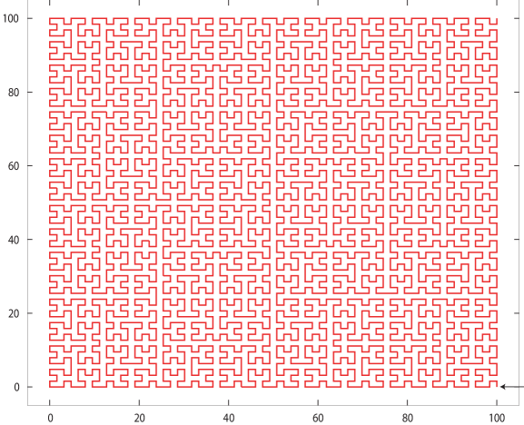
Figure 1: Hilbert Trajectory

To shed light on the anchor placement effect on localization accuracy, consider a Hilbert traversal trajectory with different anchor placement (AP) setups in Table 1. The Hilbert trajectory is formed by the piecewise connection of $8190$ points in an $100\!\times\!100$ region (see Fig(1)). A Hilbert trajectory (HT hereafer) has a space-filling property. As a result, the localization performance obtained on a HT is a good approximation to that of the underlying area.

We conduct an experiment as follows: start from the upper-left corner, the MN moves along the HT. At each point $p$ (the position of MN), noisy distance measurements $\widehat{d_{i}}=d_{i}+\epsilon_{i}$ from $p$ to the anchors are generated. Both LSM and GDM are then used to derive the estimated position. To avoid artifacts, for a given AP and noise level, the error statistics in Table 1 are obtained by traversing the HT $10$ times. Each HT traversal involves the establishment of $8190$ positions using both LSM and GDM (GDM uses the estimated position derived from LSM as its iteration initial value), with a step size of $0.00001$. The termination condition of GDM is set as $||p^{(i+1)}\!-\!p^{(i)}||_{2}\!<\!0.001$ and the maximum number of iterations is set as $100$.

TABLE 1: Anchor placement & localization accuracy

Least-Square Method
positions of anchors	$\sigma$	ave	std	time
$(0,100),(0,0),(100,0)$	$0.3$	$0.42$	$0.26$	$2.52$
	$1.0$	$1.40$	$0.85$	$2.54$
$(0,100),(7,50),(3,40)$	$0.3$	$4.01$	$3.65$	$2.51$
	$1.0$	$13.45$	$12.15$	$2.57$
Gradient Descent Method
positions of anchors	$\sigma$	ave	std	time
$(0,100),(0,0),(100,0)$	$0.3$	$0.37$	$0.21$	$63$
	$1.0$	$1.22$	$0.69$	$81$
$(0,100),(7,50),(3,40)$	$0.3$	$0.76$	$0.92$	$275$
	$1.0$	$2.94$	$7.41$	$293$
Gaussian noise ${\cal N}(0,\sigma^{2})$

The ave and std fields in Table 1 denote average localization error and standard deviation, and the time field the elapsed time per HT traversal (seconds). Table 1 shows that AP $(0,100),(0,0),(100,0)$ yields a much better localization accuracy than AP $(0,100),(7,50),(3,40)$ for both LSM and GDM. This indicates, a fortiori, that an anchor placement (AP) has a significant bearing on localization accuracy over an area. This observation raises a question: can we quantify the impact of an anchor placement (AP) with respect to an area? The aim of this paper is to answer this question.

3 Anchor Placement Effect Quantification

The section focuses on the effect quantification of anchor placement. Our main device is based on the notion of the geometric dilution of precision (GDOP) [18, 17, 22, 8]. We begin with the anchor-pair GDOP function as follows:

Theorem 1

Let $p_{i}$ and $p_{j}$ be the positions of anchor pair $i$ and $j$, and $d_{i}$ and $d_{j}$ be the actual distances from MN at $p=(x,y)$ to the anchors $i,j$, then the geometric dilution of precision at $p$ with respect to $p_{i},p_{j}$, denoted by the anchor-pair GDP function $g_{2}(p_{i},p_{j})(p)$, is

$$g_{2}(p_{i},p_{j})(p)=\sqrt{\frac{2}{1-\left(\frac{d_{i}^{2}+d_{j}^{2}-||p_{i}-p_{j}||^{2}}{2d_{i}d_{j}}\right)^{2}}},$$ (5)

where $||p_{i}\!-\!p_{j}||$ is the distance between $p_{i}=(x_{i},y_{i})$ and $p_{j}=(x_{j},y_{j})$.

Proof: Let $h(p_{i},p_{j})(p)$ be a matrix defined as

$$h(p_{i},p_{j})(p) \!=\!\begin{pmatrix}\sin(\alpha)&\cos(\alpha)\\ \sin(\beta)&\cos(\beta)\end{pmatrix}$$ (6)

$$=\!\begin{pmatrix}\frac{(x-x_{i})}{\sqrt{(x-x_{i})^{2}+(y-y_{i})^{2}}},&\frac{(y-y_{i})}{\sqrt{(x-x_{i})^{2}+(y-y_{i})^{2}}}\\ \frac{(x-x_{j})}{\sqrt{(x-x_{j})^{2}+(y-y_{j})^{2}}},&\frac{(y-y_{j})}{\sqrt{(x-x_{j})^{2}+(y-y_{j})^{2}}}\end{pmatrix},$$

where $(\sin(\alpha),\cos(\alpha))$ and $(\sin(\beta),\cos(\beta))$ denote the direction cosines from $p$ to anchors at $p_{i}$ and $p_{j}$. The anchor-pair GDOP function $g_{2}(p_{i},p_{j})(p)$ is

$$g_{2}(p_{i},p_{j})(p)=\sqrt{tr((h^{T}h)^{-1})},$$ (7)

where $T/tr$ denotes the transpose/trace of a matrix, and $A^{-1}$ refers to the inversion of $A$. A simple manipulation obtains $det(h^{T}h)=\sin^{2}(\beta-\alpha)$ and

$$g_{2}(p_{i},p_{j})(p)=\sqrt{tr((h^{T}h)^{-1})}=\sqrt{\frac{2}{\sin^{2}(\beta-\alpha)}}.$$ (8)

Substituting $\sin^{2}(\beta-\alpha)\!=1-\!(\dfrac{d_{i}^{2}+d_{j}^{2}-||p_{i}-p_{j}||^{2}}{2d_{i}d_{j}})^{2}$ into (8) yields (5). $\square$

Theorem 1 asserts that $\beta-\alpha$ degree separation represents the effect of anchor pair at $p_{i},p_{j}$ on the localization accuracy at $p$. It implies that $\beta-\alpha=\pi/2$ degree separation ($g_{2}(p_{i},p_{j})(p)=\sqrt{2}$) are best in localization accuracy, whereas $\beta-\alpha=0$ degree separation (colinear) ($g_{2}(p_{i},p_{j})(p)=\infty$) are worst. The smaller the $g_{2}(p_{i},p_{j})(p)$, the better the accuracy of localization. This is a well-known result also obtained in [22, 4, 5, 2, 8].

We now extend the anchor-pair GDOP function into the multi-anchor GDOP function. Let $p_{1},\cdots,p_{m}$ be a set of positions of anchors accessible to MN at $p$. The multi-anchor GDOP function $g_{m}(p_{1},\cdots,p_{m})(p)$ is linked to the anchor-pair GDOP function as follows:

$$g_{m}(p_{1},\cdots,p_{m})(p)=\min_{\begin{subarray}{c}1\leq i,j\leq m\\ i\not=j\end{subarray}}g_{2}(p_{i},p_{j})(p)$$ (9)

We call an anchor pair $(p_{i},p_{j})$ the optimally selected anchor pair (OSAP) if $g_{2}(p_{i},p_{j})(p)$ has a minimum value among all anchor pairs from from $p_{1},\cdots,p_{m}$. (9) shows that $g_{m}(p_{1},\cdots,p_{m})(p)$ is determined by the OSAP, which in turn varies with $p$ and accessible anchors.

Figs(3)-(3) visualize $g_{3}(\cdots)(p)$ function under the two anchor placements over the $100\times 100$ region. A three-dimensional graph in Figs(3)-(3), which is called the least vulnerability tomography (LVT), geometrizes the anchor placement effect: the LVT elevation has an implication: when in a trough area, the noise has less impact on localization accuracy than when in a peak area. Fig(3) shows that the LVT of AP $(100,0),(0,0),(0,100)$ has terrain waves with a elevation variation from $\sqrt{2}$ to $2$. In contrast, the LVT of AP $(0,100),(7,50),(3,40)$ shown in Fig(3) is relatively flat for the most part of the region but has a dramatic elevation variation from $2$ to $16$ in the vicinity of $(0,0)$ and $(0,100)$. Overall, the terrain waves in Fig(3) has a much higher elevation than that in Fig(3). This offers an explanation: why AP $(0,100),(0,0),(100,0)$ outperforms AP $(0,100),(7,50),(3,40)$ as shown in Table 1.

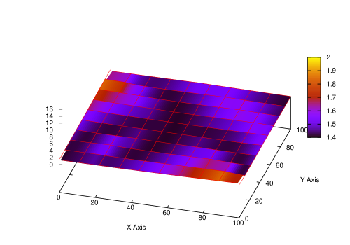
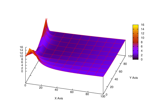
Figure 2: LVT of anchor placement $(0,100),(0,0),(100,0)$

Figure 3: LVT of anchor placement $(0,100),(7,50),(3,40)$

The LVTs in Figs(3)-(3) induce us to extend the GDOP function from a point into an area. Let $g_{m}(p_{1},\cdots,p_{m})(\Omega)$ denote the average elevation of $g_{m}(p_{1},\cdots,p_{m})(p)$ over $\Omega$. The relation between $g_{m}(p_{1},\cdots,p_{m})(\Omega)$ and $g_{m}(p_{1},\cdots,p_{m})(p)$ ($g_{m}(p_{1},\cdots,p_{m})(x,y)$) becomes

$$g_{m}(p_{1},\cdots,p_{m}) (\Omega)=\dfrac{1}{|\Omega|}\int_{\Omega}g_{m}(p_{1},\cdots,p_{m})(x,y)dx\,dy$$ (10)

Similarly, the notion of $g_{m}(p_{1},\cdots,p_{m})(p)$ can be extended from a point $p$ to a trajectory $\Gamma$ as

$$g_{m}(p_{1},\cdots,p_{m})(\Gamma) =\frac{1}{|\Gamma|}\int_{\Gamma}g_{m}(p_{1},\cdots,p_{m})(x,y)dl$$ (11)

The discrete form of (11) becomes

$$g_{m}(p_{1},\cdots,p_{m})(\Gamma)=\frac{\sum\limits_{1\leq k\leq n}g(p_{1},\cdots,p_{m})(x(t_{k}),y(t_{k}))}{n}.$$ (12)

(10) provides a means for quantifying the impact of an AP over an area. In practice, due to the arbitrariness of the area boundary and of an anchor placement, it would be impossible to derive a closed-form expression. In this paper, we use Trapezium rule method to compute (10). It is done by first splitting the area into $10,000$ non-overlapping sub-areas, then applying the Trapezium rule on each of these sub-areas.

TABLE 2: Anchor Placement Impact Quantification

Anchor Placement
$p_{1}=(0,100),p_{2}=(0,0),p_{3}=(100,0),p_{4}=(7,50),p_{5}=(3,40)$
Anchor Placement Impact over $\Omega$
$g_{3}(p_{1},p_{2},p_{3})(\Omega)$	$g_{3}(p_{1},p_{4},p_{5})(\Omega)$
$1.501$	$2.615$
Anchor Placement Impact over $\Gamma$
$g_{3}((p_{1},p_{2},p_{3})(\Gamma)$	$g_{3}(p_{1},p_{4},p_{5})(\Gamma)$
$1.499$	$2.622$
$\Omega$: $100\times 100$ area,$\Gamma$: HT

Table 2 provides a numerical calculation of AP impact over $\Omega$ and over $\Gamma$. The AP impact calculated in Table 2 implies that the localization accuracy over the $AP_{1}$ is better than that under $AP_{2}$ as $g_{3}(p_{1},p_{2},p_{3})(\Omega)<g_{3}(p_{1},p_{4},p_{5})(\Omega)$, which agree with the results obtained in noisy environments in Table 1. Comparing $g_{3}(p_{1},p_{2},p_{3})(\Omega)$ and $g_{3}(p_{1},p_{2},p_{3})(\Gamma)$ in Table 2 shows that the difference between them is very small. However, computation of $g_{3}(p_{1},p_{2},p_{3})(\Omega)$ takes about $23$ seconds, as opposed to $0.2$ seconds in computing $g_{3}(p_{1},p_{2},p_{3})(\Gamma)$.

4 Two-Phase Localization Algorithm

It is clear from Fig(3) that $g_{m}(p_{1},\cdots,p_{m})(p)$ is determined by an OSAP and the OSAP varies by area. Fig(4) shows the OSAP areas under AP $(0,100),(0,0),(100,0)$. Observe the noise-free scenario in the left-hand side graph in Fig(4) where each colored area represents an anchor pair chosen over its two alternatives based on (9). The white colored areas represent the regions in which the anchor pair at $(0,100),(0,0)$ is chosen. The blue colored areas represent the regions where the anchor pair at $(0,0),(100,0)$ has its geometric advantage over its alternative anchor pairs. The red colored areas represent the regions where the anchor pair at $(100,0),(0,100)$ is expected to produce the most accurate localization. The right-hand side graph in Fig(4) plots the OSAP areas under the noise level of $\sigma=1.0$. The presence of noise makes the borderlines on different colored areas rough and unsmooth. This is because that borderlines correspond to the isolines by two anchor pairs and hence are highly sensitive to noise.

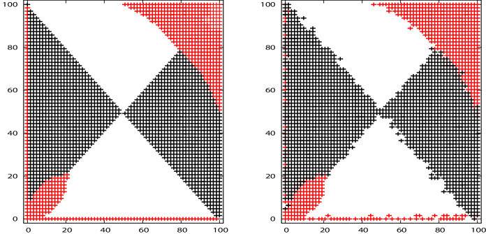
Figure 4: a) noise free b) noise level $\sigma(1.0)$: white area by anchor pair at $(0,100)\!,\!(0,0)$, black area by anchor pair at $(0,0),(100,0)$, red area by anchor pair at $(0,100)\!,\!(100,0)$

This observation of Fig(4) leads to a new two-phase localization algorithm (TPLM) that differs significantly from LSM and GDM. TMPL differs from LSM and GDM. It proceeds in two phases: In the first phase called optimal anchor pair selection, an optimal anchor pair at $(p_{i},p_{j})$ is identified based on (9), then the position(s) can be estimated by solving

$$||\widehat{p}-p_{i}||=\widehat{d_{i}},\ ||\hat{p}-p_{j}||=\widehat{d_{j}}$$ (13)

Through a lengthy manuplation, two possible solutions to (13) are obtained as follows

$$\begin{pmatrix}\widehat{x}\\ \widehat{y}\end{pmatrix}=\begin{pmatrix}\cos(\theta)&\sin(\theta)\\ \sin(\theta)&\cos(\theta)\end{pmatrix}\begin{pmatrix}u\\ v\end{pmatrix}+\begin{pmatrix}x_{i}\\ y_{i}\end{pmatrix}$$

$$\begin{pmatrix}\widehat{x}\\ \widehat{y}\end{pmatrix}=\begin{pmatrix}\cos(\theta)&\sin(\theta)\\ \sin(\theta)&\cos(\theta)\end{pmatrix}\begin{pmatrix}u\\ -v\end{pmatrix}+\begin{pmatrix}x_{i}\\ y_{i}\end{pmatrix}$$ (14)

where $\theta=\arctan(\frac{y_{j}-y_{i}}{x_{j}-x_{i}})$, $d_{ij}=||p_{i}-p_{j}||$, and

$$u=\frac{(d_{ij}^{2}+\widehat{d_{i}}^{2}-\widehat{d_{j}}^{2})}{2d_{ij}},\ v=\sqrt{d_{i}^{2}-\left(\frac{d_{ij}^{2}+\widehat{d_{i}}^{2}-\widehat{d_{j}}^{2}}{2d_{ij}}\right)^{2}}$$ (15)

In the second phase called disambiguation, the reference point obtained from LSM is used to single out one from two possible positions (4). It is done by choosing one position that has a shorter distance to the reference point.

Algorithm 1 Two-phase Localization Method

0:  $p_{i}=(x_{i},y_{i}),1\leq i\leq m$: $i^{th}$ anchor’s position

0:  $\bar{d_{i}}$: distance measurement from $j^{th}$ anchor to MN $p$

0:  $\breve{p}=(\breve{x},\breve{y})$: a reference point obtained via LSM

1:  $g_{min}\leftarrow\infty,p_{+}\leftarrow(0,0),p_{++}\leftarrow(0,0)$

2:  for $i=1$ to $m-1$ do

3:     for $j=i+1$ to $m$ do

4:        if $g_{2}(p_{i},p_{j})(p)<g_{min}$ then

5:           $g_{min}\leftarrow g(p_{i},p_{j})(p),(p_{+},p_{++})\leftarrow(p_{i},p_{j})$

6:        end if

7:     end for

8:  end for

9:  $d=|p_{+}-p_{++}|,d_{+}=|p-p_{+}|,d_{++}=|p-p_{++}|$

10:  $\theta=\arctan{\frac{y_{++}-y_{+}}{x_{++}-x_{+}}},u=\frac{d_{+}^{2}-d_{++}^{2}+d^{2}}{2d},v=\sqrt{d_{+}^{2}-u^{2}}$

11:  $p_{*}=(\begin{smallmatrix}\cos(\theta)&-\sin(\theta)\\ \sin(\theta)&\cos(\theta)\end{smallmatrix})\binom{u}{v}+\binom{x^{+}}{y^{+}}$

12:  $p_{**}=(\begin{smallmatrix}\cos(\theta)&-\sin(\theta)\\ \sin(\theta)&\cos(\theta)\end{smallmatrix})\binom{u}{-v}+\binom{x^{+}}{y^{+}}$

13:  if $|p_{*}-\breve{p}|<|p_{**}-\breve{p}|$ then

14:     return  $p_{*}$

15:  end if

16:  return  $p_{**}$

The code between lines 2-8 examines each anchor pair in turn and chooses an optimal anchor pair, which corresponds to (9). The complexity is $\binom{m}{2}$. Lines 2-12 constitute the basic block of the optimal anchor selection phase. The code between lines 13-16 is used to disambiguate the two possible solutions using the reference position $\breve{p}$ obtained by LSM.

TABLE 3: Two-Phase Localization Method

positions of anchors	$\sigma$	ave	std	time
$(0,100),(0,0),(100,0)$	$0.3$	$0.40$	$0.22$	$3.17$
	$1.0$	$1.32$	$0.73$	$3.17$
$(0,100),(7,50),(3,40)$	$0.3$	$0.70$	$0.88$	$3.44$
	$1.0$	$2.76$	$5.67$	$3.15$
Gaussian noise ${\cal N}(0,\sigma^{2})$

We present the results of TPLM in Table 3 using the same anchor placement setups in Table 1. In all cases, TPLM gives a significant error reduction over LSM with a minor degradation as TPLM uses the reference point obtained from LSM. It is fairly clear that TPLM is an order of magnitude faster than GDM, and performs slightly better than GDM in terms of localization accuracy.

5 Simulation Study

The aim of this section is threefold: first, to conduct the performance comparison between TPLM, LSM, and GDM in noise environments; second, to study the impact of noise models; and third, to investigate the random anchor placement impact.

5-A Visualizing Noise-induced Distortion

To visualize the difference among LSM, GDM, and TPLM, we plot the restored HT by LSM, GDM, and TPLM under Gaussian noise model in Figs(5)-(7) using $AP_{4}$ in Table 4. Notice that anchor positions are plotted as solid black circles.

TABLE 4: Anchor Placement Setup

Anchor Position
$p_{1}=(0,100),p_{2}=(7,50),p_{3}=(0,0)$
$p_{4}=(3,40),p_{5}=(100,0),p_{6}=(1,98)$
Anchor Placement Setup
$AP_{1}$	$(0,100),(0,0),(100,0)$
$AP_{2}$	$(0,100),(7,50),(3,40)$
$AP_{3}$	$(0,100),(0,0),(100,0),(1,98)$
$AP_{4}$	$(0,100),(7,50),(3,40),(1,98)$

Figure 5: restored HT by LSM: a) noise $(0.02)$; b) noise $(0.2)$

Figure 6: restored HT by GDM: a) noise $(0.02)$; b) noise $(0.2)$

Figure 7: restored HT by TPLM: a) noise $(0.02)$; b) noise $(0.2)$

Visual inspection reveals the apparent perceived difference among the restored HTs by LSM, GDM and TPLM: when the noise level $\sigma$ is $0.2$, the restored HT by LSM becomes completely unrecognizable in Fig(5)(b). While in Fig(6)(b) the upper right portion of the restored HT by GDM to some degree preserves the hallmark of the HT, but the most part of the recovered HT is severely distorted and barely recognizable. The restored curve by TPLM contrasts sharply with those by LSM and GDM in its preservation of fine details of the HT for the most part, while having minor distortion in the lower- and upper-left corner areas in Fig(7)(b). Such spatially uneven localization performance can be explained by examining Fig(3), which shows that the lower- and upper-left areas exactly correspond to the LVT peak areas. The perceived differences between GDM and TPLM in Figs(5)-(7) can be quantified as follows: GDM has the average error of $0.69$ per HT traversal, while TPLM produces the average error of $0.465$. In addition, GDM takes about $218.48$ seconds per HT traversal, in contrast to $2.94$ seconds taken by TPLM.

5-B Gaussian Noise vs. Non-Gaussian Noise

In this subsection, we will compare the performance of GDM and TPLM under Gaussian and uniform noise models, there are some scenarios where ranging noise may follow uniform model [7, 20]. In the experimental study, the performance between GDM and TPLM is compared under a same noise level with the different noise models. For Gaussian noise model ${\cal N}(0,\sigma^{2})$, $\sigma$ refers to the noise level in Fig(8), and for a uniform noise model $U(-a,a)$, the noise level in Fig(9) is expressed as $a^{2}/3$. The data presented reflects the average error of GDM and TPLM over $10$ HT traversals under the anchor placements in Table 2.

Figure 8: Accuracy: (top) GDM; (bottom) TPLM (Gaussian noise)

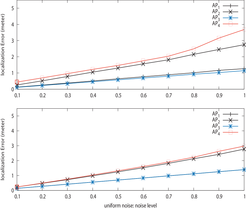
Figure 9: Accuracy: (top) GDM; (bottom) TPLM (uniform noise)

The graphs in Figs(8)-(9) represent the localization error curves of GDM and of TPLM, respectively. Under both the noise models, TPLM outperforms GDM by huge margins under $AP_{2}$ and $AP_{4}$. Both GDM and TPLM perform indistinguishably under $AP_{1}$ and $AP_{3}$. While the impact difference between $AP_{1}$ and $AP_{3}$ is barely noticed as their performance curves are overlapped, the performance curves between $AP_{1}$ and $AP_{2}$ and between $AP_{3}$ and $AP_{4}$ are clearly separated, thus the impact difference $AP_{1}$ and $AP_{2}$ and between $AP_{3}$ and $AP_{4}$ are evident.

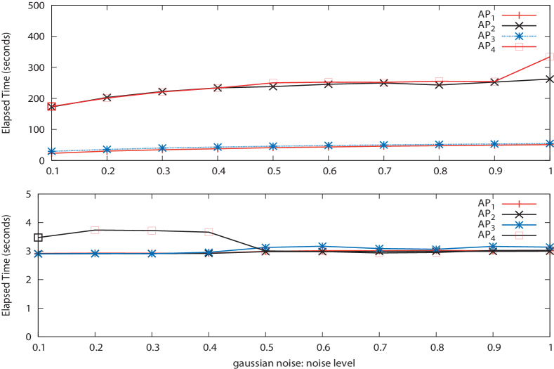
Figure 10: Elapsed time: (top) GDM; (bottom) TPLM (normal noise)

The results show that the Gaussian noise has more impact on GDM than the uniform one. By comparison, the performance of TPLM is insensitive to noise models. Fig(10) plots the elapsed time by GDM and TPLM per HT traversal, showing that TPLM is orders of magnitude faster than GDM.

5-C Random Anchor Placement

We study the impact of random anchor placement on the performance of LSM, GDM and TLPM. To achieve this, the number of anchors are randomly placed in $100\times 100$ and $50\times 100$ regions. For each randomly generated anchor placement (RGAP) in a region, the $g_{m}(p_{1},\cdots,p_{m})(\Gamma)$ function is calculated, and the error statistics of LSM, GDM, and TPLM under Gaussian noise level of $0.3$ are gathered and compared.

Fig(11)(a)-(b) show the actual $g_{m}(p_{1},\cdots,p_{m})(\Gamma)$ (average LVT elevation over $\Gamma)$) distribution by $100$ RGAPs. In the top graph, $3$ anchors are randomly placed (r.u.p.) in the entire traversal area while in the bottom graph $3$ anchors are r.u.p. in the upper half of the traversal area. Fig(11)(a) clearly exhibit positive skewness. This implies that a RGAP over the entire traversal area in general yields good localization accuracy. Recall that the smaller $g_{m}(p_{1},\cdots,p_{m})(\Gamma)$ is, the better localization is. The $g_{m}(p_{1},\cdots,p_{m})(\Gamma)$ distribution in Fig(11)(b) is more dispersed than that in the Fig(11)(a), meaning that a RGAP over the half traversal area in general underperforms a RGAP over the entire traversal area.

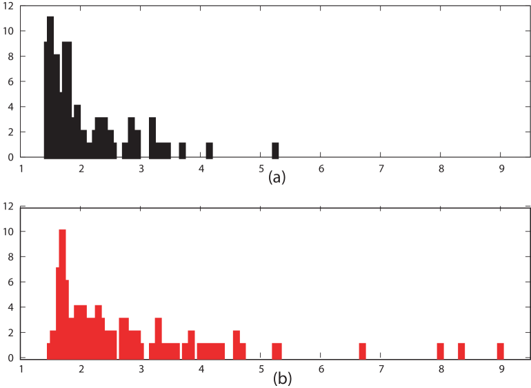
Figure 11: (a) $g_{3}(...)(\Gamma)$ distribution by $100$ RGAPs with 3 anchors in $100\times 100$; (b) $g_{3}(...)(\Gamma)$ distribution by $100$ RGAPs with 3 anchors in $50\times 100$

TABLE 5: Random Anchor placement

Random Anchor Placement in The Traversal Area
Anchors	$\overline{g_{m}(p_{1},..p_{m})(\Gamma)}$	TPLM	LSM	GDM
		ave	ave	ave
$3$	$2.05$	$0.57$	$1.52$	$0.87$
$4$	$1.69$	$0.44$	$0.79$	$0.49$
$5$	$1.53$	$0.40$	$0.59$	$0.38$
$6$	$1.48$	$0.39$	$0.51$	$0.33$
Random Anchor Placement in the Half Traversal Area
Anchors	$\overline{g_{m}(p_{1},..p_{m})(\Gamma)}$	TPLM	LSM	GDM
		ave	ave	ave
$3$	$2.72$	$0.97$	$2.82$	$1.54$
$4$	$1.93$	$0.52$	$1.37$	$0.69$
$5$	$1.77$	$0.46$	$0.81$	$0.46$
$6$	$1.69$	$0.44$	$0.72$	$0.40$

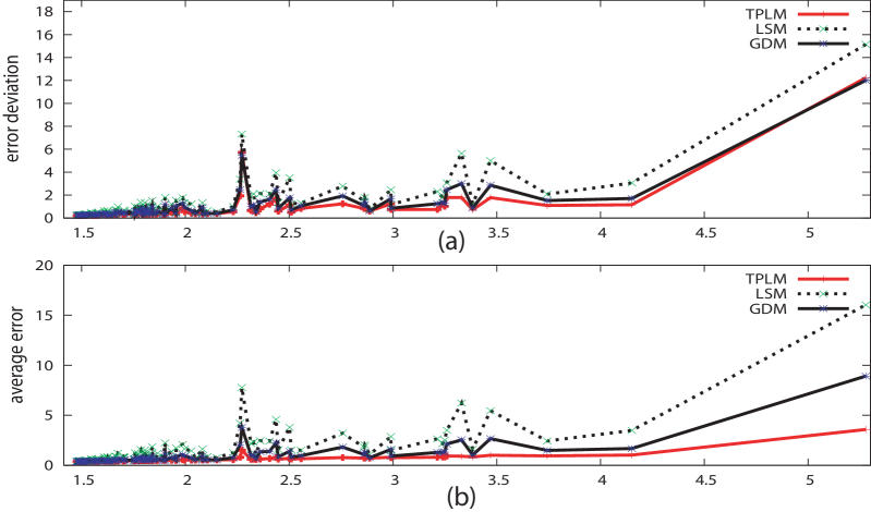
Figure 12: (a) error deviation; (b) average error (100 RGAPs with 3 anchors over the $100\times 100$ region, $\sigma=0.3$)

Fig(12) presents the performance curves of LSM, GDM, and TPLM under RGAPs, where the $x$ axis refers to the value of $g_{m}(p_{1},..p_{m})(\Gamma)$ and the $y$ axis the error deviation and average error. As is clear from Fig(12), TPLM outperforms both LSM and GDM in localization accuracy and reliability: both the error deviation and average error curves of TPLM are consistently lower than those of LSM and GDM.

Table 5 tabulates the results of RGAPs with different number of anchors, where $\overline{g_{m}(p_{1},..,p_{m})(\Gamma)}$ denotes the average $g_{m}(p_{1},..p_{m})(\Gamma)$ over $100$ RGAPs with a fixed number of anchors. It shows that the localization accuracy of TPLM over GDM is diminished as the number of anchors increases. It becomes evident that under the noise level of $0.3$, the actual performance of LSM, GDM, and TPLM deteriorates as the value of $\overline{g_{m}(p_{1},..,p_{m})(\Gamma)}$ increases. This solidifies the fact that $g_{m}(p_{1},..p_{m})(\Gamma)$ is an effective discriminator for the anchor placement impact on localization performance.

6 Field Experimental Study

This section focuses on the field test of a DARPA-sponsored research project, using the UWB-based ranging technology from Multispectrum Solutions (MSSI) [10]. and Trimble differential GPS (DGPS). Our field testbed area was a $100\times 100$ square meters. It consisted of an outdoor space largely occupied by surface parking lots and an indoor space inside a warehouse. This testbed area was further divided into $10,000$ non-overlapping $1\times 1$ grids. Each grid represents the finest positioning resolution to evaluate RF signal variation.

TABLE 6: Field testbed area and anchor placement

$x_{0}^{\prime}$	$y_{0}^{\prime}$	$x_{f}$	$y_{f}$	$\alpha$
$-74.476069$	$40.537808$	$84719$	$111045$	$0.381583$
Anchor placement
GPS position		transformed position
$-74.475585$	$40.538468$	$p_{4}=(65.345179,52.75145)$
$-74.475287$	$40.53856$	$p_{5}=(92.580022,52.83239)$
$-74.475186$	$40.538294$	$p_{6}=(89.52274,22.232383)$

In the field test, DGPS devices were mainly used for outdoor positioning while MSSI UWB-based devices were used for indoor positioning. The experimental system was composed of four MNs equipped with both the Trimble DGPS and MSSI UWB-based ranging devices. Three UWB devices were used as anchors being placed at known fixed positions. Using the known positions of the UWB anchors and real-time distance measurements, each MN could establish the current position as well as that of other MNs locally, at a rate of approximately $2$ samples per second. Each MN could also establish the position via the DGPS unit at a rate of $1$ sample per second when residing in the outdoor area. The field test area was divided into four slightly overlapping traversal quadrants denoted as $(\Gamma_{0},\Gamma_{1},\Gamma_{2},\Gamma_{3})$. A laptop (MN) equipped with DGPS and UWB ranging devices was placed in a modified stroller as shown in Fig(13), and one tester pushed the stroller, traveling along a predefined trajectory inside a quadrant (see Fig(14)). Each run lasted about $30$ minutes of walk.

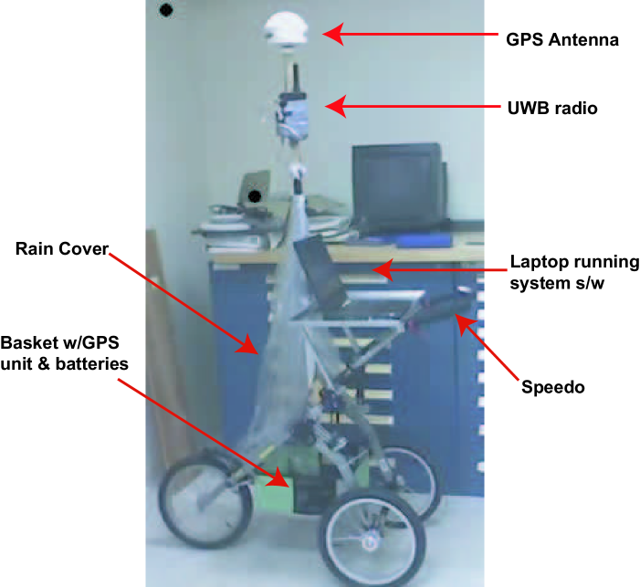
Figure 13: Stroller with a laptop attached with DGPS and UWB ranging devices

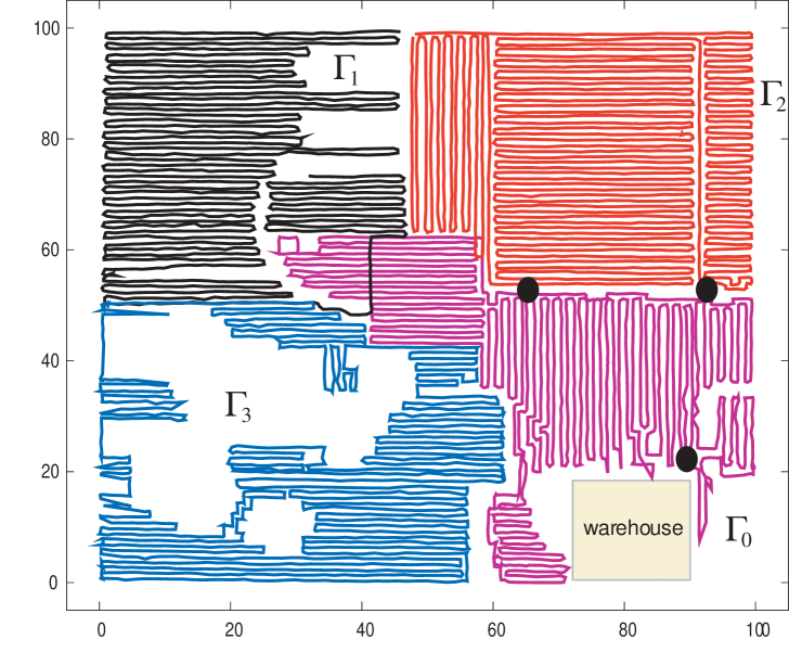
Figure 14: Four trajectories ($\Gamma_{0},\Gamma_{1},\Gamma_{2},\Gamma_{3}$), black circles: the positions of anchors, yellow rectangle: warehouse

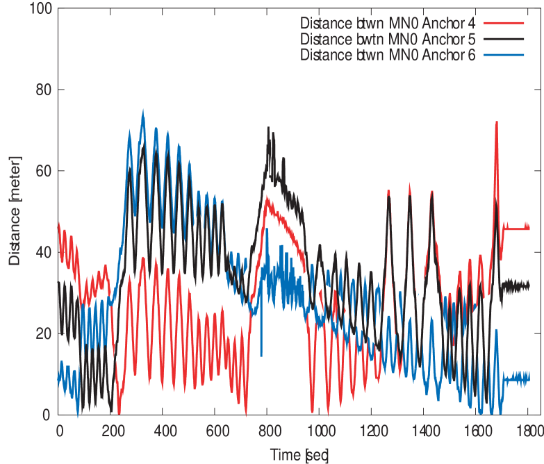
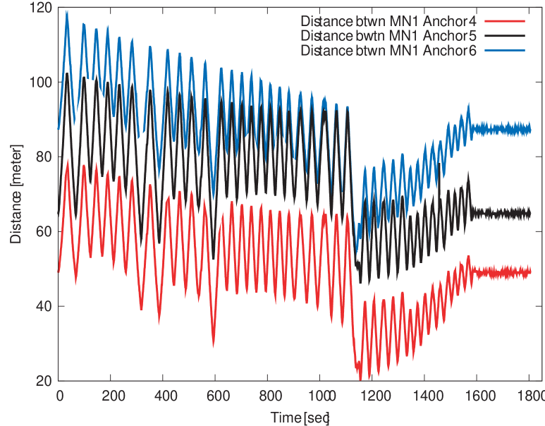
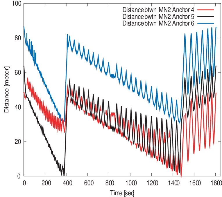
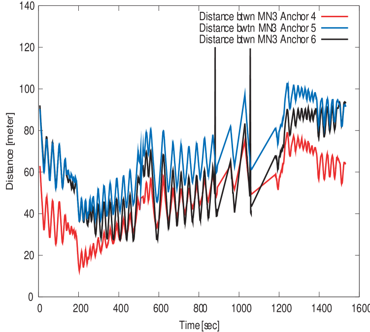
(a)	(b)	(c)	(d)

Figure 15: Distance measurements to three UWB anchors: (a) $\Gamma_{0}$, (b) $\Gamma_{1}$, (c) $\Gamma_{2}$, (d) $\Gamma_{3}$

With repeated trial runs, we found that the UWB signal could barely penetrate one cement wall of the warehouse. To establish positions inside the warehouse, we placed one anchor close to the main entrance of the warehouse while placing two other anchors around the center of the field testbed area. Fig(14) showed the four trajectories ($\Gamma_{0},\Gamma_{1},\Gamma_{2},\Gamma_{3}$) in the field test, which are translated from the GPS trajectories. A part of $\Gamma_{0}$ trajectory was inside the warehouse, thus the part of GPS of $\Gamma_{0}$ was not available. Table 7 provides the calculated results of $g_{3}(p_{4},p_{5},p_{6})(\Gamma)$ using the GPS trajectory data, indicating that $\Gamma_{0}$ would yield the most accurate localization while $\Gamma_{1}$ produced the least accurate localization.

TABLE 7: $g_{3}(p_{4},p_{5},p_{6})(\Gamma)$ of trajectories in field testbed

$g_{3}(p_{4},p_{5},p_{6})(\Gamma_{0})$	$g_{3}(p_{4},p_{5},p_{6})(\Gamma_{1})$
$1.667025$	$1.967605$
$g_{3}(p_{4},p_{5},p_{6})(\Gamma_{2})$	$g_{3}(p_{4},p_{5},p_{6})(\Gamma_{3})$
$1.787370$	$1.835048$

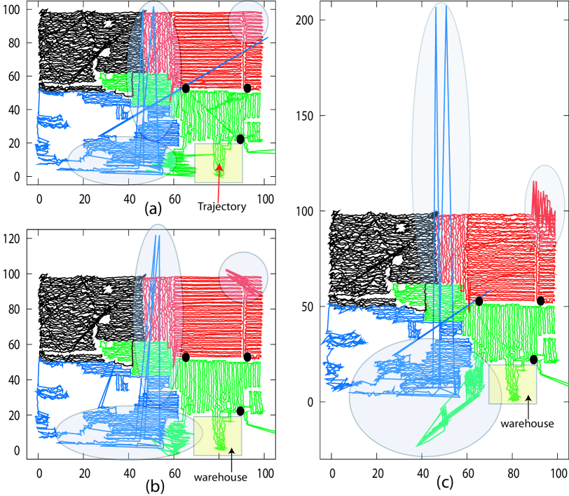
Figure 16: Restored Trajectories by (a) TPLM, (b) GDM, (c) LSM (black circles: positions of UWB anchors)

In the field testbed, the trajectory of each MN was controlled by an individual tester during a $30$-minute walk. For purpose of the primary experiment being conducted, the strollers were fitted with bicycle speedometers to allow the tester to control his speed, in order to produce sufficient reproducibility for the primary experiment, but not for our testing of localization. Due to inherent variability in each individual movement, an objective assessment of localization accuracy without a ground truth reference is almost impossible. For a performance comparison, we used GPS trajectories as a reference for visual inspection of the restored trajectories by LSM, GDM, and TPLM.

Three curves in Fig(15)(a)-(d) represent the field distance measurements between a tester and the three UWB anchor devices during a $30$-minute walk in trajectories $(\Gamma_{0},\Gamma_{1},\Gamma_{2},\Gamma_{3})$. it is fairly obvious that measurement noise in different trajectories vary widely: The distance measurement curves in trajectories $(\Gamma_{0},\Gamma_{3})$ are discontinuous and jumpy in Figs(15)(a)&(d), in contrast to the relatively smooth distance curves in trajectories $(\Gamma_{1},\Gamma_{2})$ in Fig(15)(b)&(c). Such a discontinuity in measurements occurred when testers were traveling in an area where UWB devices on stroller had no direct line of sight to UWB anchors, thus introducing additional noise in $\Gamma_{0},\Gamma_{3}$.

Figs(16)(a)-(c) show the restored trajectories by TPLM, GDM, and LSM using the UWB ranging technology in the field test. A visual inspection suggests that LSM was extremely prone to noise as its restored trajectories were appreciably distorted beyond recognition in some parts. As indicated in Fig(16)(b), GDM gave an obvious error reduction over LSM but at the expense of computational cost. The most visually perceived difference between LSM and GDM can be seen in the circled areas in Figs(16)(b)-(c). By contrast, the difference between GDM and TPLM can be visualized in the circled areas Figs(16)(a)-(b) where TPLM produced a detail-preserved but slightly distorted contour of the trajectory. A further offline analysis showed that on average GDM takes $18.87ms$ per position establishment, while TPLM/LSM take $0.4/0.35ms$.

7 Conclusion

This paper studies the geometric effect of anchor placement on localization performance. The proposed approach allows the construction of the least vulnerability tomography (LVT) for comparing the geometric impact of different anchor placements. As a byproduct, we propose a two-phase localization method.

To validate theoretical results, we conduct comprehensive simulation experiments based on randomly generated anchor placements and different noise models. The experimental results agree with our anchor placement impact analysis. In addition, we show that TPLM outperforms LSM by a huge margin in accuracy. TPLM performs much faster than GDM and slightly better than GDM in localization accuracy. The field study shows that TPLM is more robust against noise than LSM and GDM.

In this paper, we adopt a widely used assumption that measurement noise is independent of distance. This assumption is somewhat unrealistic in some practical settings. In our future research, we will perform experiments using UWB ranging technology to study the noise-distance relation in indoor and outdoor environments. The anchor placement impact analysis will be refined to incorporate more realistic noise-distance models.

References

- [1] G.B. Arfken and H.J. Weber. Mathematical Methods for Physicists, Sixth Edition: A Comprehensive Guide. Academic Press, 2005.
- [2] A.N. Bishop, B. Fidan, B.D.O Anderson, K. Dogancay, and N. Pathirana. Optimality analysis of sensor-target geometries in passive location: Part 1- bearing-only localization. In ISSNIP, September 2007.
- [3] A.N. Bishop, B. Fidan, B.D.O. Anderson, K. Dogancay, and P.N. Pathirana. Optimality analysis of sensor-target localization geometries. Automatic, 46(3), 2010.
- [4] A.N. Bishop and P Jensfelt. Optimality analysis of sensor-target geometries in passive location: Part 2- time-of-arrival based localization. In ISSNIP, September 2007.
- [5] A.N. Bishop and P Jensfelt. An optimality analysis of sensor-target geometries for signal strength based localization. In ISSNIP, September 2009.
- [6] J. Bruck, J. Gao, and A. Jiang. Localization and routing in sensor network by local angle information. ACM Trans. on Sensor Networks, 5(1), February 2009.
- [7] N. Bulusu, J. Heidemann, and D. Estrin. Adaptive beacon placement. In The 21th International Conference on Distributed Computing Systems, April 2001.
- [8] S. O. Dulman, A. Baggio, P.J.M. Havinga, and K.G. Langendoen. A geometrical perspective on localization. In the 14th Annual International Conference on Mobile Computing and Networking, 2008.
- [9] T. Eren, D.K. Goldenberg, W. Whiteley, Y. R. Yang, A. S. Morse, D. O. Anderson, and P. N. Belhumeur. Rigidity, computation, and randomization in network localization. In INFOCOM, pages 2673–2684, March 2004.
- [10] R. J. Fontana. Recent system applications of short-pulse ultra-wideband technology. IEEE Trans. on Microwave Theory and Techniques, 52(9):2087–2104, September 2004.
- [11] S. Gezici, Z. Tian, G.B. Giannakis, H. Kobayashi, A.F. Molisch, H.V. Poor, and Z. Sahinoglu. Localization via ultra-wideband radios. IEEE Signal Processing Mag, 22(4), 2005.
- [12] A. Kannan, B. Fidan, and G. Mao. Derivation of flip ambiguity probabilities to facilitate robust sensor network localization. In IEEE Wireless Communications and Networking Conference, 2009.
- [13] A. Kannan, B. Fidan, and G. Mao. Analysis of flip ambiguities for robust sensor network localization. IEEE Trans. on Vehicular Technology, 59(4), 2010.
- [14] K. Langendoen and N. Reijers. Distributed Localization Algorithms. In R. Zurawski, editor, Embedded Systems Handbook. CRC press, August 2005.
- [15] S. Lederer, Y. Wang, and J. Gao. Connectivity-based localization of large scale sensor networks with complex shape. In INFOCOM, May 2008.
- [16] S. Lederer, Y. Wang, and J. Gao. Connectivity-based localization of large scale sensor networks with complex shape. ACM Trans. on Sensor Networks, 5(4), November 2009.
- [17] H.B. Lee. Accuracy limitation of hyperbolic multilateration systems. IEEE Trans. on Aerospace and Electronic Systems, AES-11, January 1975.
- [18] H.B. Lee. A novel procedure for assessing the accuracy of hyperbolic multilateration systems. IEEE Trans. on Aerospace and Electronic Systems, AES-11, January 1975.
- [19] Z. Li, W. Trappe, Y. Zhang, and B. Nath. Robust statistical methods for securing wireless localization in sensor networks. In IPSN, 2005.
- [20] L. Liu and M.G. Amin. Performance analysis of gps receivers in non-gaussian noise incorporating precorrelction filter and sampling rate. IEEE. Trans. On Signal Processing, 56(3), March 2008.
- [21] D. Moore, J. Leonard, D. Rus, and S. Teller. Robust Distributed Network Localization with Noisy Range Measurements. In Proceeding of SenSys’04, November 2004.
- [22] N. Patwari, J.N. Ash, S. Kyperountas, A.O. Hero III, R.L. Moses, and N.S. Correal. Locating the Nodes: Cooperative localization in wireless sensor networks. IEEE Signal Process. Mag, 22(4), 2005.
- [23] N.B. Priyantha, H. Balakrishnan, E. Demaine, and S. Teller. Anchor-free Distributed Localization in Sensor Networks. In Tech Report #892, MIT Laboratory for Compter Science, April 2003.
- [24] A.M. So and Y. Ye. Theory of semidefinite programming for sensor network localization. In SODA, 2005.
- [25] R. Stoleru, T. He, and J.A. Stankovic. Walking GPS: A Practical Solution for Localization in Manually Deployed Wireless Sensor Networks. In Proceedings of IEEE Workshop on Embedded Networked Sensors, November 2004.
- [26] P. Tseng. Second-order cone programming relaxation of sensor network localization. SIAM J. Optim, 18, 2007.
- [27] K. Whitehouse and D. Culler. A robustness analysis of multi-hop ranging-based localozation approximations. In IPSN, 2006.
- [28] K. Whitehouse, C. Karlof, A. Woo, F. Jiang, and D. Culler. The effects of ranging noise on multihop localozation: an empirical study. In IPSN, 2005.
- [29] M. Youssef and A. Agrawala. Towards an Optimal Strategy for WLAN Location Determination Systems. International Journal of Modelling and Simulation, 27, 2007.
- [30] G. Zhao, T. He, and J. A. Stankovic. Impact of Radio Asymmetry on Wireless Sensor Networks. In Proceedings of ACM Conference on Embedded Networked Sensor Systems, November 2004.