Positive-P phase space method simulation in superradiant emission from a cascade atomic ensemble

Abstract

The superradiant emission properties from an atomic ensemble with cascade level configuration is numerically simulated. The correlated spontaneous emissions (signal then idler fields) are purely stochastic processes which are initiated by quantum fluctuations. We utilize the positive-P phase space method to investigate the dynamics of the atoms and counter-propagating emissions. The light field intensities are calculated, and the signal-idler correlation function is studied for different optical depths of the atomic ensemble. Shorter correlation time scale for a denser atomic ensemble implies a broader spectral window needed to store or retrieve the idler pulse.

I Introduction

A quantum communication network based on the distribution and sharing of entangled states is potentially secure to eavesdropping and is therefore of great practical interest QI ; cryp ; QI2 .  A protocol for the realization of such a long distance system, known as the quantum repeater, was proposed by Briegel et al. repeater ; Dur .  A quantum repeater based on the use of atomic ensembles as memory elements, distributed over the network, was subsequently suggested by Duan, Lukin, Cirac and Zoller dlcz .  The storage of information in the atomic ensembles involves the Raman scattering of an incident light beam from ground state atoms with the emission of a signal photon.  The photon is correlated with the creation of a phased, ground-state, coherent excitation of the atomic ensemble.  The information may be retrieved by a reverse Raman scattering process, sending the excitation back to the initial atomic ground state and generating an idler photon directionally correlated with the signal photon qubit ; chou ; vuletic ; collective ; store ; collective2 ; single2 ; pan ; kimble .  In the alkali gases, the signal and the idler field wavelengths are in the near-infrared spectral region.  This presents a wavelength mismatch with telecommunication wavelength optical fiber, which has a transmission window at longer wavelengths (1.1-1.6 um).  It is this mismatch that motivates the search for alternative processes that can generate telecom wavelength photons correlated with atomic spin waves telecom .

This motivates the research presented in this article where we study multi-level atomic schemes in which the transition between the excited states is resonant with a telecom wavelength light field telecom .  The basic problem is to harness the absorption and the emission of telecom photons while preserving quantum correlations between the atoms, which store information and the photons that carry along the optical fiber channel of the network.

It is not common to have a telecom ground state transition in atomic gases except for rare earth elements erbium ; dysprosium or in an erbium-doped crystal solid .  However, a telecom wavelength (signal) can be generated from transitions between excited levels in the alkali metals telecom ; radaev .

The ladder configuration of atomic levels provides a source for telecom photons (signal) from the upper atomic transition.  For rubidium and cesium atoms, the signal field has the range around 1.3-1.5 $\mu$m that can be coupled to an optical fiber and transmitted to a remote location.  Cascade emission may result in pairs of photons, the signal entangled with the subsequently emitted infrared photon (idler) from the lower atomic transition.  Entangled signal and idler photons were generated from a phase-matched four-wave mixing configuration in a cold, optically thick ⁸⁵Rb ensemble telecom .  This correlated two-photon source is potentially useful as the signal field has telecom wavelength.

The temporal emission characteristics of the idler field, generated on the lower arm of the cascade transition, were observed in measurements of the joint signal-idler correlation function.  The idler decay time was shorter than the natural atomic decay time and dependent on optical thickness in a way reminiscent of superradiance Dicke ; Stephen ; Lehm ; mu ; OC:Mandel .

The spontaneous emission from an optically dense atomic ensemble is a many-body problem due to the radiative coupling between atoms.  This coupling is responsible for the phenomenon of superradiance firstly discussed by Dicke Dicke in 1954.

Since then, this collective emission has been extensively studied in two atom systems indicating a dipole-dipole interaction Stephen ; Lehm , in the totally inverted N atom systems stehle ; Tallet , and in the extended atomic ensemble mu .  The emission intensity has been investigated using the master equation approach master ; Bon ; Bon1 and with Maxwell-Bloch equations Bon2 ; Feld .  A useful summary and review of superradiance can be found in the reference Gross ; phase .  Recent approaches to superradiance include the quantum trajectory method trajectory ; eig1 and the quantum correction method Fleischhauer99 .

In the limit of single atomic excitation, superradiant emission characteristics have been discussed in the reference Eberly and Scully .  For a singly excited system, the basis set reduces to N rather than $2^{N}$ states.  Radiative phenomena have been investigated using dynamical methods kurizki ; Scully2 ; eig2 and by the numerical solution of an eigenvalue problem Friedberg08a ; Svidzinsky08 ; Friedberg08b ; Friedberg08c .  A collective frequency shift Arecchi ; Morawitz can be significant at a high atomic density Scully09 and has been observed recently in an experiment where atoms are resonant with a planar cavity supershift .

To account for multiple atomic excitations in the signal-idler emission from a cascade atomic ensemble, the Schrödinger’s equation approach becomes cumbersome.  An alternative theory of c-number Langevin equations is suitable for solution by stochastic simulations.

Langevin equations were initially derived to describe Brownian motion SM:Gardiner .  A fluctuating force is used to represent the random impacts of the environment on the Brownian particle.  A given realization of the Langevin equation involves a trajectory perturbed by the random force.  Ensemble averaging such trajectories provides a natural and direct way to investigate the dynamics of the stochastic variables.

An essential element in the stochastic simulations is a proper characterization of the Langevin noises.  These represent the quantum fluctuations responsible for the initiation of the spontaneous emission from the inverted Feld ; Haake1 ; Haake2 ; Polder79 , or pumped atomic system Chiao88 ; Chiao95 as in our case.

The positive-P phase space method QN:Gardiner ; quantization ; Smith88 ; Smith0 ; Smith1 ; Boyd89 ; Drummond91 is employed to derive the Fokker-Planck equations that lead directly to the c-number Langevin equations.  The classical noise correlation functions, equivalently diffusion coefficients, are alternatively confirmed by use of the Einstein relations LP:Sargent ; QO:Scully ; Fleischhauer94 .  The c-number Langevin equations correspond to Ito-type stochastic differential equations that may be simulated numerically.  The noise correlations can be represented either by using a square Carmichael86 or a non-square ”square root” diffusion matrix Smith1 .  The approach enables us to calculate normally-ordered quantities, signal-idler field intensities, and the second-order correlation function.  The numerical approach involves a semi-implicit difference algorithm and shooting method numerical to integrate the stochastic ”Maxwell-Bloch” equations.

Recently a new positive-P phase space method involving a stochastic gauge function Drummond02 has been developed.  This approach has an improved treatment of sampling errors and boundary errors in the treatment of quantum anharmonic oscillators Drummond01 ; Collett01 .  It has also been applied to a many-body system of bosons Drummond03 and fermions Drummond06 .  In this paper, we follow the traditional positive-P representation method drummond80 .

The remainder of this paper is organized as follows. In section II, we show the formalism of positive P-representation, and demonstrate the stochastic differential equations of cascade emission (signal and idler) from an atomic ensemble. In section III we solve numerically for the dynamics of the atoms and counter-propagating signal and idler fields in a positive P-representation. We present results of signal and idler field intensities, and the signal-idler second order correlation function for different optical depths of the atomic ensemble. Section IV presents our discussions and conclusions. In the appendix, we show the details in the derivations of c-number Langevin equations that are the foundation for numerical approaches of the cascade emission.  In Appendix A, we formulate the Hamiltonian, and derive the Fokker-Planck equations by characteristic functions LT:Haken in positive P-representation. Then corresponding c-number Langevin equations are derived, and the noise correlations are found from the diffusion coefficients in Fokker-Planck equations as shown in Appendix B.

II Theory of Cascade emission

The phase space methods QN:Gardiner that mainly include P-, Q-, and Wigner (W) representations are techniques of using classical analogues to study quantum systems, especially harmonic oscillators.  The eigenstate of harmonic oscillator is a coherent state that provides the basis expansion to construct various representations.  P and Q-representation are associated respectively with evaluations of normal and anti-normal order correlations of creation and destruction operators.  W-representation is invented for the purpose of describing symmetrically ordered creation and destruction operators.  Since P-representation describes normally ordered quantities that are relevant in experiments, we are interested in investigating one class of generalized P-representations, the positive P-representation that has semi-definite property in the diffusion process, which is important in describing quantum noise systems.

Positive-P representation QO:Walls ; drummond80 is an extension to Glauber-Sudarshan P-representation that uses coherent state ($|\alpha\rangle$) as a basis expansion of density operator $\rho$.  In terms of diagonal coherent states with a quasi-probability distribution, $P(\alpha,\alpha^{\ast})$, a density operator in P-representation is

$$\rho=\int_{D}|\alpha\rangle\langle\alpha|P(\alpha,\alpha^{\ast})d^{2}\alpha,$$ (1)

where $D$ represents the integration domain.  The normalization condition of $\rho,$ which is Tr{$\rho$}$=1,$ indicates the normalization for $P$ as well, $\int_{D}P(\alpha,\alpha^{\ast})d^{2}\alpha=1$.

Positive P-representation uses a non-diagonal coherent state expansion and the density operator can be expressed as

$$\rho=\int_{D}\Lambda(\alpha,\beta)P(\alpha,\beta)d\mu(\alpha,\beta),$$ (2)

where

$$d\mu(\alpha,\beta)=d^{2}\alpha d^{2}\beta\text{ and }\Lambda(\alpha,\beta)=\frac{|\alpha\rangle\langle\beta^{\ast}|}{\langle\beta^{\ast}|\alpha\rangle},$$ (3)

and $\langle\beta^{\ast}|\alpha\rangle$ in non-diagonal projection operators, $\Lambda(\alpha,\beta),$ makes sure of the normalization condition in distribution function, $P(\alpha,\beta).$

Any normally ordered observable can be deduced from the distribution function $P(\alpha,\beta)$ that

$$\langle(a^{{\dagger}})^{m}a^{n}\rangle=\int_{D}\beta^{m}\alpha^{n}P(\alpha,\beta)d\mu(\alpha,\beta).$$ (4)

A characteristic function $\chi_{p}(\lambda_{\alpha},\lambda_{\beta})$ (Fourier-transformed distribution function in Glauber-Sudarshan P-representation but now is extended into a larger dimension) can help formulate distribution function, which is

$$\chi_{p}(\lambda_{\alpha},\lambda_{\beta})=\int_{D}e^{i\lambda_{\alpha}\alpha+i\lambda_{\beta}\beta}P(\alpha,\beta)d\mu(\alpha,\beta).$$ (5)

It is calculated from a normally ordered exponential operator $E(\lambda),$

$$\chi_{p}(\lambda_{\alpha},\lambda_{\beta})=\text{Tr\{}\rho E(\lambda)\text{\}, }E(\lambda)=e^{i\lambda_{\beta}a^{\dagger}}e^{i\lambda_{\alpha}a}.$$ (6)

Then a Fokker-Planck equation can be derived from the time derivative of characteristic function,

$$\frac{\partial\chi_{p}}{\partial t}=\frac{\partial}{\partial t}\text{Tr\{}\rho E(\lambda)\text{\}=Tr\{}\frac{\partial\rho}{\partial t}E(\lambda)\text{\}}$$ (7)

by Liouville equations,

$$\frac{\partial\rho}{\partial t}=\frac{1}{i\hbar}[H,\rho].$$ (8)

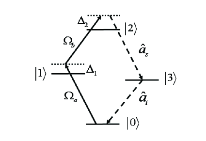
Figure 1: Four-level atomic ensemble interacting with two driving lasers (solid) with Rabi frequencies $\Omega_{a}$ and $\Omega_{b}.$  Signal and idler fields are labelled by $\hat{a}_{s}$ and $\hat{a}_{i},$ respectively and $\Delta_{1}$ and $\Delta_{2}$ are one and two-photon laser detunings.

In laser theory LT:Haken , a P-representation method is extended to describe atomic and atom-field interaction systems.  When a large number of atoms is considered, which is indeed the case of the actual laser, a macroscopic variable can be defined.  Then a generalized Fokker-Planck equation can be derived from characteristic functions by neglecting higher order terms that are proportional to the inverse of number of atoms.  It is similar to our case when we solve light-matter interactions in an atomic ensemble that the large number cuts off the higher order terms in characteristic functions.

We consider $N$ cold atoms that are initially prepared in the ground state interacting with four independent electromagnetic fields.  As shown in Fig.1, two driving lasers (of Rabi frequencies $\Omega_{a}$ and $\Omega_{b}$) excite a ladder configuration $|0\rangle\rightarrow|1\rangle\rightarrow|2\rangle.$  Two quantum fields, signal $\hat{a}_{s}$ and idler $\hat{a}_{i},$ are generated spontaneously. We note that the spontaneous emission from the cascade driving scheme is a stochastic process due to the quantum fluctuations, unlike the diamond configuration where quantum noise can be neglected conversion ; thesis .

The complete derivation of the c-number Langevin equations for cascade emission from the four-level atomic ensemble is described in Appendix A and B.  After setting up the Hamiltonian, we follow the standard procedure to construct the characteristic functions LT:Haken in Appendix A using the positive-P representation QN:Gardiner .  In Appendix B.1, the Fokker-Planck equation is found by directly Fourier transforming the characteristic functions, and making a $1/N_{z}$ expansion.

Finally the Ito stochastic differential equations are written down from inspection of the first-order derivative (drift term) and second-order derivative (diffusion term) in the Fokker-Planck equation.  The equations are then written in dimensionless form by introducing the Arecchi-Courtens cooperation units scale in Appendix B.2.  From Eq. (30) and the field equations that follow, these c-number Langevin equations in a co-moving frame are,

$$\frac{\partial}{\partial\tau}\pi_{01} =(i\Delta_{1}-\frac{\gamma_{01}}{2})\pi_{01}+i\Omega_{a}(\pi_{00}-\pi_{11})+i\Omega_{b}^{\ast}\pi_{02}-i\pi_{13}^{{\dagger}}E_{i}^{+}+\mathcal{F}_{01}\text{ (I),}$$

$$\frac{\partial}{\partial\tau}\pi_{12} =i(\Delta_{2}-\Delta_{1}+i\frac{\gamma_{01}+\gamma_{2}}{2})\pi_{12}-i\Omega_{a}^{\ast}\pi_{02}+i\Omega_{b}(\pi_{11}-\pi_{22})+i\pi_{13}E_{s}^{+}e^{-i\Delta kz}+\mathcal{F}_{12},$$

$$\frac{\partial}{\partial\tau}\pi_{02} =(i\Delta_{2}-\frac{\gamma_{2}}{2})\pi_{02}-i\Omega_{a}\pi_{12}+i\Omega_{b}\pi_{01}+i\pi_{03}E_{s}^{+}e^{-i\Delta kz}-i\pi_{32}E_{i}^{+}+\mathcal{F}_{02},$$

$$\frac{\partial}{\partial\tau}\pi_{11} =-\gamma_{01}\pi_{11}+\gamma_{12}\pi_{22}+i\Omega_{a}\pi_{01}^{{\dagger}}-i\Omega_{a}^{\ast}\pi_{01}-i\Omega_{b}\pi_{12}^{{\dagger}}+i\Omega_{b}^{\ast}\pi_{12}+\mathcal{F}_{11},$$

$$\frac{\partial}{\partial\tau}\pi_{22} =-\gamma_{2}\pi_{22}+i\Omega_{b}\pi_{12}^{{\dagger}}-i\Omega_{b}^{\ast}\pi_{12}+i\pi_{32}^{{\dagger}}E_{s}^{+}e^{-i\Delta kz}-i\pi_{32}E_{s}^{-}e^{i\Delta kz}+\mathcal{F}_{22},$$

$$\frac{\partial}{\partial\tau}\pi_{33} =-\gamma_{03}\pi_{33}+\gamma_{32}\pi_{22}-i\pi_{32}^{{\dagger}}E_{s}^{+}e^{-i\Delta kz}+i\pi_{32}E_{s}^{-}e^{i\Delta kz}+i\pi_{03}^{{\dagger}}E_{i}^{+}-i\pi_{03}E_{i}^{-}+\mathcal{F}_{33},$$

$$\frac{\partial}{\partial\tau}\pi_{13} =-(i\Delta_{1}+\frac{\gamma_{01}+\gamma_{03}}{2})\pi_{13}-i\Omega_{a}^{\ast}\pi_{03}-i\Omega_{b}\pi_{32}^{{\dagger}}+i\pi_{12}E_{s}^{-}e^{i\Delta kz}+i\pi_{01}^{{\dagger}}E_{i}^{+}+\mathcal{F}_{13},$$

$$\frac{\partial}{\partial\tau}\pi_{03} =-\frac{\gamma_{03}}{2}\pi_{03}-i\Omega_{a}\pi_{13}+i\pi_{02}E_{s}^{-}e^{i\Delta kz}+i(\pi_{00}-\pi_{33})E_{i}^{+}+\mathcal{F}_{03},$$

$$\frac{\partial}{\partial\tau}\pi_{32} =i\Delta_{2}-\frac{\gamma_{03}+\gamma_{2}}{2}\pi_{32}+i\Omega_{b}\pi_{13}^{{\dagger}}-i(\pi_{22}-\pi_{33})E_{s}^{+}e^{-i\Delta kz}-i\pi_{02}E_{i}^{-}+\mathcal{F}_{32},$$

$$\frac{\partial}{\partial z}E_{s}^{+} =-i\pi_{32}e^{i\Delta kz}\frac{|g_{s}|^{2}}{|g_{i}|^{2}}-\mathcal{F}_{s},\text{ }\frac{\partial}{\partial z}E_{i}^{+}=i\pi_{03}+\mathcal{F}_{i},$$ (9)

where (I) stands for Ito type SDE.  $\pi_{ij}$ is the stochastic variable that corresponds to the atomic populations of state $|i\rangle$ when $i=j$ and to atomic coherence when $i\neq j$, and $\mathcal{F}_{ij}$ are c-number Langevin noises.  The remaining equations of motion, which close the set, can be found by replacing the above classical variables, $\pi_{jk}^{\ast}\rightarrow\pi_{jk}^{{\dagger}},$ $(\pi_{jk}^{{\dagger}})^{\ast}\rightarrow\pi_{jk},$ $(E_{s,i}^{+})^{\ast}\rightarrow E_{s,i}^{-},$ $(E_{s,i}^{-})^{\ast}\rightarrow E_{s,i}^{+}$ , and $\mathcal{F}_{jk}^{\ast}\rightarrow\mathcal{F}_{jk}^{{\dagger}}$.  Note that the atomic populations satisfy $\pi_{jj}^{\ast}=\pi_{jj}.$  The superscripts, dagger (${\dagger}$) for atomic variables and ($-$) for field variables, denote the independent variables, which is a feature of the positive-P representation: there are double dimension spaces for each variable.  These variables are complex conjugate to each other when ensemble averages are taken, for example $\left\langle\pi_{jk}\right\rangle=\left\langle\pi_{jk}^{{\dagger}}\right\rangle^{\ast}$ and $\left\langle E_{s,i}^{+}\right\rangle=\left\langle E_{s,i}^{-}\right\rangle^{\ast}.$  The doubled spaces allow the variables to explore trajectories outside the classical phase space.

Before going further to discuss the numerical solution of the SDE, we point out that the diffusion matrix elements have been computed using Fokker-Planck equations and by the Einstein relations discussed in Appendix B.2.  This provides the important check on the lengthy derivations of the diffusion matrix elements we need for the simulations.

The next step is to find expressions for the Langevin noises in terms of a non-square matrix $B$ QO:Walls ; Smith1 .  The matrix $B$ is used to construct the symmetric diffusion matrix $D(\alpha)=B(\alpha)B^{T}(\alpha)$ for a Ito SDE,

$$dx_{t}^{i}=A_{i}(t,\overrightarrow{x_{t}})dt+\sum\limits_{j}B_{ij}(t,\overrightarrow{x_{t}})dW_{t}^{j}(t)\text{ \ (I)}$$ (10)

where $\xi_{i}dt=dW_{t}^{i}(t)$ (Wiener process) and $\left\langle\xi_{i}(t)\xi_{j}(t^{\prime})\right\rangle=\delta_{ij}\delta(t-t^{\prime}).$  Note that $B\rightarrow BS,$ where $S$ is an orthogonal matrix ($SS^{T}=I$), leaves $D$ unchanged, so $B$ is not unique.  We could also construct a square matrix representation $B$ QN:Gardiner ; SM:Gardiner ; Carmichael86 .  This involves a procedure of matrix decomposition into a product of lower and upper triangular matrix factors.  A Cholesky decomposition can be used to determine the $B$ matrix elements successively row by row.  The downside of this procedure is that the $B$ matrix elements must be differentiated in converting the Ito SDE to its equivalent Stratonovich form for numerical solution.

The Stratonovich SDE is necessary for the stability and the convergence of semi-implicit methods.  Because of the analytic difficulties in transforming to the Stratonovich form, we use instead the non-square form of $B$ Smith1 .

In this case a typical $B$ matrix element is a sum of terms, each one of which is a product of the square root of a diffusion matrix element with a unit strength real (if the diffusion matrix element is diagonal) or complex (if the diffusion matrix element is off-diagonal) Gaussian unit white noise.  It is straightforward to check that a $B$ matrix constructed in this way reproduces the required diffusion matrix $D=BB^{T}$.

As pointed out in the reference Drummond91 , the transverse dipole-dipole interaction can be neglected and nonparaxial spontaneous decay rate can be accounted for by a single atom decay rate if the atomic density is not too high.  We are interested here in conditions where the ensemble length $L$ is significant and propagation effects are non-negligible, and the average distance between atoms $d=\sqrt[3]{V/N}$ is larger than the transition wavelength $\lambda.$  The length scales satisfy $\lambda\lesssim d\ll L,$ and we consider a pencil-like cylindrical atomic ensemble.  The paraxial or one-dimensional assumption for field propagation is then valid, and the transverse dipole-dipole interaction is not important for the atomic density we focus here.

The theory of cascade emission presented here provides the solid ground for simulations of fluctuations that initiate the radiation process in the atomic ensemble. A proper way of treating fluctuations or noise correlations and formulating SDE requires an Ito form that is derived from the Fokker-Planck equation. An alternative but more straightforward approach by making quantum to classical correspondence in the quantum Langevin equation does not guarantee an Ito type SDE. That is the reason we take the route of Fokker-Planck equation, and the coupled equations of Eq.(9) are the main results in this section.

III Results for signal, idler intensities, and the second-order correlation function

There are several possible ways to integrate the differential equation numerically.  Three main categories of algorithm used are forward (explicit), backward (implicit), and mid-point (semi-implicit) methods numerical . The forward difference method, which Euler or Runge-Kutta methods utilizes, is not guaranteed to converge in stochastic integrations xmds .  There it is shown that the semi-implicit method semi is more robust in Stratonovich type SDE simulations Drummond91b .  More extensive studies of the stability and convergence of SDE can be found in the reference SDE:Kloeden .  The Stratonovich type SDE equivalent to the Ito type equation (10), is

$$dx_{t}^{i} =[A_{i}(t,\overrightarrow{x_{t}})-\frac{1}{2}\sum\limits_{j}\sum\limits_{k}B_{jk}(t,\overrightarrow{x_{t}})\frac{\partial}{\partial x^{j}}B_{ik}(t,\overrightarrow{x_{t}})]dt$$

$$+\sum\limits_{j}B_{ij}(t,\overrightarrow{x_{t}})dW_{t}^{j}\text{ \ (Stratonovich),}$$ (11)

which has the same diffusion terms $B_{ij},$ but with modified drift terms.  This ”correction” term arises from the different definitions of stochastic integral in the Ito and Stratonovich calculus.

At the end of Appendix C.3, we derive the ”correction” terms noted above.  We then have 19 classical variables including atomic populations, coherences, and two counter-propagating cascade fields.  With 64 diffusion matrix elements and an associated 117 random numbers required to represent the instantaneous Langevin noises, we are ready to solve the equations numerically using the robust midpoint difference method.

The problem we encounter here involves counter-propagating field equations in the space dimension and initial value type atomic equations in the time dimension. The counter-propagating field equations have a boundary condition specified at each end of the medium.  This is a two-point boundary value problem, and a numerical approach to its solution, the shooting method numerical , is used here.

Any normally-ordered quantity $\left\langle Q\right\rangle$ can be derived by ensemble averages that $\left\langle Q\right\rangle=\sum_{i=1}^{R}Q_{i}/R$ where $Q_{i}$ is the result for each realization.

In this section, we present the second-order correlation function of signal-idler fields, and their intensity profiles.   We define the intensities of signal and idler fields by

$$I_{s}(t)=\left\langle E_{s}^{-}(t)E_{s}^{+}(t)\right\rangle,\text{ }I_{i}(t)=\left\langle E_{i}^{-}(t)E_{i}^{+}(t)\right\rangle,$$ (12)

respectively, and the second-order signal-idler correlation function

$$G_{s,i}(t,\tau)=\left\langle E_{s}^{-}(t)E_{i}^{-}(t+\tau)E_{i}^{+}(t+\tau)E_{s}^{+}(t)\right\rangle$$ (13)

where $\tau$ is the delay time of the idler field with respect a reference time $t$ of the signal field.  Since the correlation function is not stationary QL:Loudon , we choose $t$ as the time when $G_{s,i}$ is at its maximum.

We consider a cigar shaped ⁸⁵Rb ensemble of radius $0.25$ mm and $L=3$ mm.  The operating conditions of the pump lasers are ($\Omega_{a},$ $\Omega_{b},$ $\Delta_{1},$ $\Delta_{2}$) $=$ ($0.4,$ $1,$ $1,$ $0$)$\gamma_{03}$ where $\Omega_{a}$ is the peak value of a $50$ ns square pulse, and $\Omega_{b}$ is the Rabi frequency of a continuous wave laser. Four-wave mixing condition ($\Delta k=0$) is assumed. The four atomic levels are chosen as ($|0\rangle,$ $|1\rangle,$ $|2\rangle,$ $|3\rangle$) $=$ ($|$5S${}_{1/2},$F=3$\rangle,$ $|5$P${}_{3/2},$F=4$\rangle,$ $|4$D${}_{5/2},$F=5$\rangle,$ $|5$P${}_{3/2},$F=4$\rangle$).  The natural decay rate for atomic transition $|1\rangle\rightarrow|0\rangle$ or $|3\rangle\rightarrow|0\rangle$ is $\gamma_{01}=\gamma_{03}=1/26$ ns and they have a wavelength 780 nm.  For atomic transition $|2\rangle\rightarrow|1\rangle$ or $|2\rangle\rightarrow|3\rangle$ is $\gamma_{12}=\gamma_{32}=0.156\gamma_{03}$ gsgi with a telecom wavelength 1.53$\mu$m.  The scale factor of the coupling constants for signal and idler transitions is $g_{s}/g_{i}=0.775.$

We have investigated six different atomic densities from a dilute ensemble with an optical density (opd) of 0.01 to a opd = 8.71.  In Fig.2, 3, and 4, we take the atomic density $\rho=10^{10}$ cm^-3 (opd = 2.18) for example, and the grid sizes for dimensionless time $\Delta t=4$ and space $\Delta z=0.0007$ are chosen.  The convergence of the grid spacings is fixed in practice by convergence to the signal intensity profile with an estimated relative error less than 0.5%.

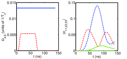
Figure 2: (Color online) Time-varying pump fields and time evolution of atomic populations. (Left) The first pump field $\Omega_{a}$ (dotted-red) is a square pulse of duration 50 ns and $\Omega_{b}$ is continuous wave (solid-blue).  (Right) The time evolution of the real part of populations for three atomic levels $\sigma_{11}=\left\langle\tilde{\alpha}_{13}\right\rangle$ (dash dotted-red), $\sigma_{22}=\left\langle\tilde{\alpha}_{12}\right\rangle$ (dotted-blue), $\sigma_{33}=\left\langle\tilde{\alpha}_{11}\right\rangle$ (solid-green) at $z=0,L$, and almost vanishing imaginary parts for all three of them. indicate convergence of the ensemble averages. Note that these atomic populations are uniform as a function of $z.$

The temporal profiles of the exciting lasers are shown in the left panel of Fig.2.  The atomic density is chosen as $\rho=10^{10}$ cm${}^{-3},$ and the cooperation time $T_{c}$ is 0.35 ns.  The right panel shows time evolution of atomic populations for levels $|1\rangle$, $|2\rangle,$ and $|3\rangle$ at $z=0,L,$ that are spatially uniform.  The populations are found by ensemble averaging the complex stochastic population variables.  The imaginary parts of the ensemble averages tend to zero as the ensemble size is increased, and this is a useful indicator of convergence.  In this example, the ensemble size was 8$\times 10^{5}.$  The small rise after the pump pulse $\Omega_{a}$ is turned off is due to the modulation caused by the pump pulse $\Omega_{b},$ which has a generalized Rabi frequency $\sqrt{\Delta_{2}^{2}+4\Omega_{b}^{2}}$. This influences also the intensity profiles and the correlation functions.

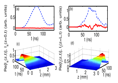
Figure 3: (Color online) Spatial-temporal intensity profiles of counter-propagating signal and idler fields.  (a) At $z=0,$ real (dashed-blue) and imaginary (solid-red) parts of signal intensity.  (b) At $z=L,$ real (dash dotted-blue) and imaginary (solid-red) parts of idler intensity.  (c) and (d) are spatial-temporal profiles for signal and idler intensities respectively.  Both intensities are normalized by the peak value of signal intensity that is $7.56\times 10^{-12}$ $E_{c}^{2}$.  Note that the idler fluctuations and its non-vanishing imaginary part indicate a relatively slower convergence compared with the signal intensity.  The ensemble size was 8$\times 10^{5},$ and the atomic density $\rho=10^{10}$cm^-3.

In Fig.3, we show counter-propagating signal ($-\hat{z}$) and idler ($+\hat{z}$) field intensities at the respective ends of the atomic ensemble and their spatial-temporal profiles respectively.  The plots show the real and imaginary parts of the observables, and both are normalized to the peak value of signal intensity.  Note that the characteristic field strength in terms of natural decay rate of the idler transition ($\gamma_{03}$) and dipole moment ($d_{i}$) is $(d_{i}/\hbar)E_{c}\approx 36.3\gamma_{03}$.  The fluctuation in the real idler field intensity at $z=L$ and non-vanishing imaginary part indicates a slower convergence compared to the signal field that has an almost vanishing imaginary part.  The slow convergence is a practical limitation of the method.

In Fig.4 (a), we show a contour plot of the second-order correlation function $G_{s,i}(t_{s},t_{i})$ where $t_{i}\geq t_{s}.$  In Figure 4 (b), a section is shown through $t_{s}\approx 75$ ns where $G_{s,i}$ is at its maximum.  The approximately exponential decay of $G_{s,i}$ is clearly superradiant qualitatively consistent with the reference telecom .  The non-vanishing imaginary part of $G_{s,i}$ calculated by ensemble averaging is also shown in (b) and indicates a reasonable convergence after 8$\times 10^{5}$ realizations.

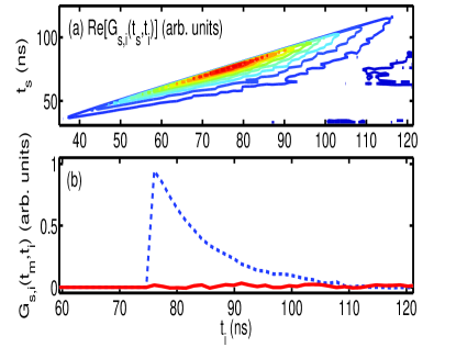
Figure 4: (Color online) Second-order correlation function $G_{s,i}(t_{s},t_{i}).$ The 2-D contour plot of the real part of $G_{s,i}$ with a causal cut-off at $t_{s}=t_{i}$ is shown in (a).  The plot (b) gives a cross-section at $t_{s}=t_{m}\approx 75$ ns, which is normalized to the maximum of the real part (dashed-blue) of $G_{s,i}.$  The imaginary part (solid-red) of $G_{s,i}$ is nearly vanishing, and the number of realizations is 8$\times 10^{5}$ for $\rho=10^{10}$cm${}^{-3}.$

In Table 1, we display numerical parameters of our simulations for six different atomic densities.  The number of dimensions in space and time is $M_{t}\times M_{z}$ with grid sizes ($\Delta t,\Delta z$) in terms of cooperation time ($T_{c}$), length ($L_{c}$).  The superradiant time scale ($T_{f}$) is found by fitting $G_{s,i}$ to an exponential function ($e^{-t/T_{f}}$), with $95\%$ confidence range.

Table 1: Numerical simulation parameters for different atomic densities $\rho$. Corresponding optical depth (opd), time and space grids ($M_{t}\times M_{z}$) with grid sizes ($\Delta t,\Delta z$) in terms of cooperation time ($T_{c}$) and length ($L_{c}$), and the fitted characteristic time $T_{f}$ for $G_{s,i}$ (see text).

$\rho($cm${}^{-3})$	opd	$M_{t}\times M_{z}$	$\Delta t(T_{c}),$ $\Delta z(L_{c})$	$T_{c}($ns$),$ $L_{c}($m$)$	fitted $T_{f}$ (ns)
5$\times 10^{7}$	$0.01$	$111\times 42$	0.3, 5$\times 10^{-5}$	4.89, 1.47	$25.9$
5$\times 10^{8}$	$0.11$	$101\times 44$	0.9, 1.5$\times 10^{-4}$	1.55, 0.46	$24.6$
5$\times 10^{9}$	$1.09$	$101\times 42$	2.8, 4.5$\times 10^{-4}$	0.49, 0.15	$14.8$
1$\times 10^{10}$	$2.18$	$101\times 42$	4.0, 7$\times 10^{-4}$	0.35, 0.10	$9.4$
2$\times 10^{10}$	$4.35$	$101\times 42$	5.5, 1$\times 10^{-3}$	0.24, 0.07	$5.0$
4$\times 10^{10}$	$8.71$	$101\times 42$	8.0, 1.4$\times 10^{-3}$	0.17, 0.06	$3.1$

In Fig.5, the characteristic time scale is plotted as a function of atomic density and the factor $N\mu$, and shows faster decay for optically denser atomic ensembles.  We also plot the timescale $T_{1}=\gamma_{03}^{-1}/(N\mu+1)$ (ns) where $\mu$ is the geometrical constant for a cylindrical ensemble mu .   The natural decay time $\gamma_{03}^{-1}=26$ ns corresponds to the D2 line of ⁸⁵Rb.  The error bar indicates the deviation due to the fitting range from the peak of $G_{s,i}$ to approximately 25% and 5% of the peak value.  The results of simulations are in good qualitative agreement with the timescale of $T_{1}$ that can be regarded as a superradiant time constant of lower transition in a two-photon cascade QO:Scully ; QL:Loudon . $T_{f}$ approaches independent atom behavior at lower densities, which indicates no collective behavior as expected. We note here that our simulations involve multiple excitations within the pumping condition similar to the experimental parameters telecom . The small deviation of $T_{f}$ and $T_{1}$ might be due to the multiple emissions considered in our simulations other than a two-photon source. On the other hand the close asymptotic dependence of atomic density or optical depth in $T_{f}$ and $T_{1}$ indicates a strong correlation between signal and idler fields due to the four-wave mixing condition as required and crucial in experiment telecom .

For larger opd atomic ensembles, larger statistical ensembles are necessary for numerical simulations to converge.  The integration of 8$\times 10^{5}$ realizations used in the case of $\rho=10^{10}$ cm^-3 consumes about 14 days with Matlab’s parallel computing toolbox (function ”parfor”) with a Dell precision workstation T7400 (64-bit Quad-Core Intel Xeon processors).

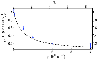
Figure 5: (Color online) Characteristic timescales, $T_{f}$ and $T_{1}$ vs atomic density $\rho$ and the superradiant enhancement factor $N\mu$. $\ T_{f}$ (dotted-blue) is the fitted characteristic timescale for $G_{s,i}(t_{s}=t_{m},t_{i}=t_{m}+\tau)$ where $t_{m}$ is chosen at its maximum, as in Figure 4.  The error bars indicate the fitting uncertainties.  As a comparison, $T_{1}$=$\gamma_{03}^{-1}/$($N\mu+1$) (dashed-black) is plotted where $\gamma_{03}^{-1}=26$ ns is the natural decay time of D2 line of ⁸⁵Rb atom, and $\mu$ is the geometrical constant for a cylindrical atomic ensemble.  The number of realizations is 4$\times 10^{5}$ for $\rho=5\times 10^{7}$, $5\times 10^{8}$, $5\times 10^{9}$ cm^-3, 8$\times 10^{5}$ for $\rho=10^{10}$, $2\times 10^{10}$ cm^-3, and 16$\times 10^{5}$ for $\rho=4\times 10^{10}$ cm^-3.

IV Discussion and Conclusion

The cascade atomic system studied here provides a source of telecommunication photons that are crucial for long distance quantum communication. We may take advantage of such low loss transmission bandwidth in the DLCZ protocol for a quantum repeater. The performance of the protocol relies on the efficiency of generating the cascade emission pair, which is better for a larger optical depth of the prepared atomic ensemble. For other applications in quantum information science such as quantum swapping and quantum teleportation, the frequency space correlations also influence their success rates spectral . To utilize and implement the cascade emission in quantum communication, we characterize the emission properties, especially the signal-idler correlation function and its dependence on optical depths. Its superradiant timescale indicates a broader spectral distribution which saturates the storage efficiency of idler pulse in an auxiliary atomic ensemble telecom by means of EIT (electromagnetic induced transparency). Therefore our calculation provides the minimal spectral window (1/$T_{f}$) of EIT to efficiently store and retrieve the idler pulse.

In summary, we have derived c-number Langevin equations in the positive-P representation for the cascade signal-idler emission process in an atomic ensemble.  The equations are solved numerically by a stable and convergent semi-implicit difference method, while the counter-propagating spatial evolution is solved by implementing the shooting method.  We investigate six different atomic densities readily obtainable in a magneto-optical trap experiment.  Signal and idler field intensities and their correlation function are calculated by ensemble averages.  Vanishing of the unphysical imaginary parts within some tolerance is used as a guide to convergence.  We find an enhanced characteristic time scale for idler emission in the second-order correlation functions from a dense atomic ensemble, qualitatively consistent with the superradiance timescales used in a cylindrical dense atomic ensemble mu ; telecom .

Appendix A Hamiltonian and Characteristic functions in Positive P-representation method

The Hamiltonian $H$ is in Schrödinger picture, and we separate it into two parts where $H_{0}$ is the free Hamiltonian of the atomic ensemble and one dimensional counter-propagating signal and idler fields, and $H_{I}$ is the interaction Hamiltonian of atoms interacting with two classical fields and two quantum fields (signal and idler) as shown in Fig.1.  Dipole approximation of $-\vec{d}\cdot\vec{E}$ and rotating wave approximation (RWA) have been made to these interactions.  Using the standard quantization of electromagnetic field quantization , we have

$$H_{0} =\sum_{i=1}^{3}\sum_{l=-M}^{M}\hbar\omega_{i}\tilde{\sigma}_{ii}^{l}+\hbar\omega_{s}\sum_{l=-M}^{M}\hat{a}_{s,l}^{{\dagger}}\hat{a}_{s,l}$$

$$+\hbar\sum_{l,l^{\prime}}\omega_{l^{\prime}l}\hat{a}_{s,l}^{{\dagger}}\hat{a}_{s,l^{\prime}}+\hbar\omega_{i}\sum_{l=-M}^{M}\hat{a}_{i,l}^{{\dagger}}\hat{a}_{i,l}$$

$$+\hbar\sum_{l,l^{\prime}}\omega_{ll^{\prime}}\hat{a}_{i,l}^{{\dagger}}\hat{a}_{i,l^{\prime}}\text{ ,}$$ (14)

$$H_{I} =-\hbar\sum_{l=-M}^{M}\Big{[}\Omega_{a}(t)\tilde{\sigma}_{01}^{l\dagger}e^{ik_{a}z_{l}-i\omega_{a}t}$$

$$+\Omega_{b}(t)\tilde{\sigma}_{12}^{l\dagger}e^{-ik_{b}z_{l}-i\omega_{b}t}+h.c.\Big{]}$$

$$-\hbar\sum_{l=-M}^{M}\Big{[}g_{s}\sqrt{2M+1}\tilde{\sigma}_{32}^{l\dagger}\hat{a}_{s,l}e^{-ik_{s}z_{l}}$$

$$+g_{i}\sqrt{2M+1}\tilde{\sigma}_{03}^{l\dagger}\hat{a}_{i,l}e^{ik_{i}z_{l}}+h.c.\Big{]}$$ (15)

where $\tilde{\sigma}_{mn}^{l}\equiv\sum_{\mu}^{N_{z}}\hat{\sigma}_{mn}^{\mu,l}=\sum_{\mu}^{N_{z}}|m\rangle_{\mu}\langle n|\Big{|}_{r_{\mu}=z_{l}},~{}\Omega_{a}(t)\equiv f_{a}(t)d_{10}\mathcal{E}(k_{a})/(2\hbar),$ and $f_{a}$ is slow varying temporal profile without spatial dependence (ensemble scale much less than pulse length). $g_{s}\equiv d_{23}\mathcal{E}(k_{s})/\hbar,~{}\mathcal{E}(k)=\sqrt{\hbar\omega/2\epsilon_{0}V}$ and $z_{m}=\frac{mL}{2M+1},~{}m=-M,...,M,$ and $L$ is the length of propagation that is equally split into $2M+1$ elements. Commutation relations of field operators are $[\hat{a}_{l},\hat{a}_{l^{\prime}}^{{\dagger}}]=\delta_{ll^{\prime}},$ and the matrix $\omega_{ll^{\prime}}\equiv\sum_{n}\frac{k_{n}c}{2M+1}e^{ik_{n}(z_{l}-z_{l^{\prime}})}$ accounts for field propagation by coupling the local mode operators where $k_{n}=2\pi n/L$.  Note that the Rabi frequency is half of the standard definition.

The normally ordered exponential operator is chosen as

$$E(\lambda) =\prod_{l}E^{l}(\lambda),$$

$$E^{l}(\lambda) =e^{i\lambda_{19}^{l}\tilde{\sigma}_{01}^{l\dagger}}e^{i\lambda_{18}^{l}\tilde{\sigma}_{12}^{l\dagger}}e^{i\lambda_{17}^{l}\tilde{\sigma}_{02}^{l\dagger}}e^{i\lambda_{16}^{l}\tilde{\sigma}_{13}^{l\dagger}}e^{i\lambda_{15}^{l}\tilde{\sigma}_{03}^{l\dagger}}e^{i\lambda_{14}^{l}\tilde{\sigma}_{32}^{l\dagger}}\times$$

$$e^{i\lambda_{13}^{l}\tilde{\sigma}_{11}^{l}}e^{i\lambda_{12}^{l}\tilde{\sigma}_{22}^{l}}e^{i\lambda_{11}^{l}\tilde{\sigma}_{33}^{l}}e^{i\lambda_{10}^{l}\tilde{\sigma}_{32}^{l}}e^{i\lambda_{9}^{l}\tilde{\sigma}_{03}^{l}}e^{i\lambda_{8}^{l}\tilde{\sigma}_{13}^{l}}\times$$

$$e^{i\lambda_{7}^{l}\tilde{\sigma}_{02}^{l}}e^{i\lambda_{6}^{l}\tilde{\sigma}_{12}^{l}}e^{i\lambda_{5}^{l}\tilde{\sigma}_{01}^{l}}e^{i\lambda_{4}^{l}\hat{a}_{s,l}^{\dagger}}e^{i\lambda_{3}^{l}\hat{a}_{s,l}}e^{i\lambda_{2}^{l}\hat{a}_{i,l}^{\dagger}}e^{i\lambda_{1}^{l}\hat{a}_{i,l}}.$$ (16)

Aside from the atom-field interaction $\frac{\partial\rho}{\partial t}=\frac{1}{i\hbar}[H,\rho],$ when dissipation from vacuum is considered (single atomic decay), we can express them in terms of a Lindblad form where we have for the four-level atomic system,

$$\big{(}\frac{\partial\rho}{\partial t}\big{)}_{sp}=$$

$$\sum_{l=-M}^{M}\sum_{\mu}^{N_{z}}\Big{\{}\frac{\gamma_{01}}{2}[2\hat{\sigma}_{01}^{\mu,l}\rho\hat{\sigma}_{01}^{\mu,l\dagger}-\hat{\sigma}_{01}^{\mu,l\dagger}\hat{\sigma}_{01}^{\mu,l}\rho-\rho\hat{\sigma}_{01}^{\mu,l\dagger}\hat{\sigma}_{01}^{\mu,l}]$$

$$+\frac{\gamma_{12}}{2}[2\hat{\sigma}_{12}^{\mu,l}\rho\hat{\sigma}_{12}^{\mu,l\dagger}-\hat{\sigma}_{12}^{\mu,l\dagger}\hat{\sigma}_{12}^{\mu,l}\rho-\rho\hat{\sigma}_{12}^{\mu,l\dagger}\hat{\sigma}_{12}^{\mu,l}]$$

$$+\frac{\gamma_{32}}{2}[2\hat{\sigma}_{{}_{32}}^{\mu,l}\rho\hat{\sigma}_{{}_{32}}^{\mu,l\dagger}-\hat{\sigma}_{{}_{32}}^{\mu,l\dagger}\hat{\sigma}_{{}_{32}}^{\mu,l}\rho-\rho\hat{\sigma}_{{}_{32}}^{\mu,l\dagger}\hat{\sigma}_{{}_{32}}^{\mu,l}]$$

$$+\frac{\gamma_{03}}{2}[2\hat{\sigma}_{03}^{\mu,l}\rho\hat{\sigma}_{03}^{\mu,l\dagger}-\hat{\sigma}_{03}^{\mu,l\dagger}\hat{\sigma}_{03}^{\mu,l}\rho-\rho\hat{\sigma}_{03}^{\mu,l\dagger}\hat{\sigma}_{03}^{\mu,l}]\Big{\}}.$$ (17)

The characteristic functions can be calculated as

$$\chi =\text{Tr\{}E(\lambda)\rho\text{\},}$$ (18)

$$\frac{\partial\chi}{\partial t} =\text{Tr\{}E(\lambda)\frac{\partial\rho}{\partial t}\text{\}}$$

$$=\big{(}\frac{\partial\chi}{\partial t}\big{)}_{A}+\big{(}\frac{\partial\chi}{\partial t}\big{)}_{L}+\big{(}\frac{\partial\chi}{\partial t}\big{)}_{A-L}+\big{(}\frac{\partial\chi}{\partial t}\big{)}_{sp},$$ (19)

$$\big{(}\frac{\partial\chi}{\partial t}\big{)}_{A} =\text{Tr\{}E(\lambda)\frac{1}{i\hbar}[H_{A},\rho]\text{\}, }$$

$$\big{(}\frac{\partial\chi}{\partial t}\big{)}_{L} =\text{Tr\{}E(\lambda)\frac{1}{i\hbar}[H_{L},\rho]\text{\},}$$

$$\big{(}\frac{\partial\chi}{\partial t}\big{)}_{A-L} =\text{Tr\{}E(\lambda)\frac{1}{i\hbar}[H_{A-L},\rho]\text{\}, }$$

$$\big{(}\frac{\partial\chi}{\partial t}\big{)}_{sp} =\text{Tr\{}E(\lambda)\big{(}\frac{\partial\rho}{\partial t}\big{)}_{sp}\text{\}}$$ (20)

where $H_{0}=H_{A}+H_{L}$, $H_{A}$ is the atomic free evolution Hamiltonian, $H_{L}$ is the Hamiltonian for laser fields, and $H_{A-L}=H_{I}.$ The detail of derivations in various characteristic functions can be found in laser theory LT:Haken or theory of light-atom interactions in atomic ensembles thesis .

Appendix B Stochastic Differential Equation

A distribution function can be found by Fourier transforming the characteristic functions,

$$f(\vec{\alpha})=\frac{1}{(2\pi)^{n}}\int...\int e^{-i\vec{\alpha}\cdot\vec{\lambda}}\chi(\vec{\lambda})d\lambda_{1}...d\lambda_{n},$$ (21)

then

$$\frac{\partial f}{\partial t}=\frac{1}{(2\pi)^{n}}\int...\int e^{-i\vec{\alpha}\cdot\vec{\lambda}}\frac{\partial\chi}{\partial t}d\lambda_{1}...d\lambda_{n}.$$ (22)

If $\frac{\partial\chi}{\partial t}=i\lambda_{\beta}\frac{\partial\chi}{\partial(i\lambda_{\gamma})}$, use integration by parts and neglect the boundary terms, we have $\frac{\partial f}{\partial t}=-\frac{\partial}{\partial(\alpha_{\beta})}\alpha_{\gamma}f$ where a minus sign is from $i\lambda_{\beta}$.  Correspondingly, if $\frac{\partial\chi}{\partial t}=e^{i\lambda_{\beta}}$, we have

$\frac{\partial f}{\partial t}=e^{-\frac{\partial}{\partial(\alpha_{\beta})}}$.

B.1 Fokker-Planck equation

Let

$$\frac{\partial f}{\partial t}=\mathcal{L}f=\sum_{l,l^{\prime}}$$

$$[\mathcal{L}_{A}\delta_{ll^{\prime}}+\mathcal{L}_{L}+\mathcal{L}_{A-L}^{(a)}\delta_{ll^{\prime}}+\mathcal{L}_{A-L}^{(b)}\delta_{ll^{\prime}}+\mathcal{L}_{sp}\delta_{ll^{\prime}}]f,$$ (23)

and we may neglect higher order derivatives (third order and higher) in various $\mathcal{L}$’s.  The validity of truncation to second order is due to the expansion in the small parameter $1/N_{z}$.

If the Fokker-Planck equation is

$$\frac{\partial f}{\partial t}=-\frac{\partial}{\partial\alpha}A_{\alpha}f-\frac{\partial}{\partial\beta}A_{\beta}f+\frac{1}{2}(\frac{\partial^{2}}{\partial\alpha\partial\beta}+\frac{\partial^{2}}{\partial\beta\partial\alpha})D_{\alpha\beta}f$$ (24)

where $A$ and $D$ are drift and diffusion terms then we have a corresponding classical Langevin equation

$$\frac{\partial\alpha}{\partial t}=A_{\alpha}+\Gamma_{\alpha}\text{, }\frac{\partial\beta}{\partial t}=A_{\beta}+\Gamma_{\beta}$$ (25)

with a correlation function $\langle\Gamma_{\alpha}\Gamma_{\beta}\rangle=\delta(t-t^{\prime})D_{\alpha\beta}$.  So now we can derive the equations of motion according to various $\mathcal{L}$’s, but we postpone them and derivations of diffusion coefficients after the scaling is made for a dimensionless form in the next subsection. The demonstration of various $\mathcal{L}$’s can be found in laser theory LT:Haken or theory of light-atom interactions in atomic ensembles thesis .

B.2 Slowly varying envelopes and scaled equations of motion

Here we introduce the slowly varying envelopes and define our cross-grained collective atomic and field observables, then finally transform the equations in a dimensionless form for later numerical simulations. Define slow varying observables that

$$\widetilde{\alpha}_{5}(z,t)\equiv\frac{1}{N_{z}}\alpha_{5}^{l}e^{-ik_{a}z_{l}+i\omega_{a}t},~{}\widetilde{\alpha}_{6}(z,t)\equiv\frac{\alpha_{6}^{l}}{N_{z}}e^{ik_{b}z_{l}+i\omega_{b}t},$$

$$\widetilde{\alpha}_{7}(z,t)\equiv\frac{1}{N_{z}}\alpha_{7}^{l}e^{-ik_{a}z_{l}+ik_{b}z_{l}+i\omega_{b}t+i\omega_{a}t},$$

$$~{}\widetilde{\alpha}_{8}(z,t)\equiv\frac{1}{N_{z}}\alpha_{8}^{l}e^{-i\omega_{a}t+i\omega_{3}t+ik_{a}z_{l}-ik_{i}z_{l}},$$

$$\widetilde{\alpha}_{9}(z,t)\equiv\frac{1}{N_{z}}\alpha_{9}^{l}e^{-ik_{i}z_{l}+i\omega_{3}t},\widetilde{\alpha}_{11}(z,t)\equiv\frac{1}{N_{z}}\alpha_{11}^{l},$$

$$\widetilde{\alpha}_{12}(z,t)\equiv\frac{1}{N_{z}}\alpha_{12}^{l},\widetilde{\alpha}_{13}(z,t)\equiv\frac{1}{N_{z}}\alpha_{13}^{l},$$

$$\text{ }\widetilde{\alpha}_{14}(z,t)\equiv\frac{1}{N_{z}}\alpha_{14}^{l}e^{-i(\omega_{23}+\Delta_{2})t}e^{ik_{a}z_{l}-ik_{b}z_{l}-ik_{i}z_{l}}$$ (26)

where $e^{i\Delta kz}=e^{ik_{a}z_{l}-ik_{b}z_{l}-ik_{i}z_{l}+ik_{s}z_{l}}$. We note that

$$i\sum_{l^{\prime}}\omega_{ll^{\prime}}\alpha_{4}^{l^{\prime}}=c\frac{d}{dz_{l}}\alpha_{4}^{l}\text{, }-i\sum_{l^{\prime}}\omega_{ll^{\prime}}\alpha_{1}^{l^{\prime}}=-c\frac{\partial}{\partial z_{l}}\alpha_{1}^{l},$$ (27)

and $\alpha_{0}^{l}=N_{z}-\alpha_{13}^{l}-\alpha_{12}^{l}-\alpha_{11}^{l}$, which will be used in later coupled equations. Also for the field variables,

$$E_{s}^{-}(z,t)\equiv\frac{g_{s}^{\ast}}{d_{i}/\hbar}\sqrt{2M+1}\alpha_{4}^{l}e^{-i\omega_{s}t},$$

$$\text{ }E_{i}^{+}(z,t)\equiv\frac{g_{i}}{d_{i}/\hbar}\sqrt{2M+1}\alpha_{1}^{l}e^{i\omega_{i}t},$$ (28)

where we use the idler dipole moment in signal field scaling for the purpose of scale-free atomic equation of motions, so we need to keep in mind that in calculating signal intensity or correlation function, an extra factor of $(d_{i}/d_{s})^{2}$ needs to be taken care of.

We choose the central frequency of signal and idler as $\omega_{s}=\omega_{23}+\Delta_{2},\omega_{i}=\omega_{3}$ where $\Delta_{1}=\omega_{a}-\omega_{1}$ and $\Delta_{2}=\omega_{a}+\omega_{b}-\omega_{2}$.  With a scaling of Arecchi-Courtens cooperation length scale , we set up the units of time, length, and field strength in the following,

$$\text{ }L_{c}=cT_{c},\text{ }\frac{1}{T_{c}}=\sqrt{\frac{d_{i}^{2}n\omega_{i}}{2\hbar\epsilon_{0}}},\text{ }E_{c}=\frac{1}{T_{c}}\frac{1}{d_{i}/\hbar}.$$ (29)

Now the slowly varying and dimensionless equations of motion with Langevin noises in Ito’s form are

$$\frac{\partial}{\partial t}\widetilde{\alpha}_{5} =(i\Delta_{1}-\frac{\gamma_{01}}{2})\widetilde{\alpha}_{5}+i\Omega_{a}(\widetilde{\alpha}_{0}-\widetilde{\alpha}_{13})+i\Omega_{b}^{\ast}\widetilde{\alpha}_{7}-i\widetilde{\alpha}_{16}E_{i}^{+}+\mathcal{F}_{5},$$

$$\frac{\partial}{\partial t}\widetilde{\alpha}_{6} =i(\Delta_{2}-\Delta_{1}+i\frac{\gamma_{01}+\gamma_{2}}{2})\widetilde{\alpha}_{6}-i\Omega_{a}^{\ast}\widetilde{\alpha}_{7}+i\Omega_{b}(\widetilde{\alpha}_{13}-\widetilde{\alpha}_{12})+i\widetilde{\alpha}_{8}E_{s}^{+}e^{-i\Delta kz}+\mathcal{F}_{6},$$

$$\frac{\partial}{\partial t}\widetilde{\alpha}_{7} =(i\Delta_{2}-\frac{\gamma_{2}}{2})\widetilde{\alpha}_{7}-i\Omega_{a}\widetilde{\alpha}_{6}+i\Omega_{b}\widetilde{\alpha}_{5}+i\widetilde{\alpha}_{9}E_{s}^{+}e^{-i\Delta kz}-i\widetilde{\alpha}_{10}E_{i}^{+}+\mathcal{F}_{7},$$

$$\frac{\partial}{\partial t}\widetilde{\alpha}_{13} =-\gamma_{01}\widetilde{\alpha}_{13}+\gamma_{12}\widetilde{\alpha}_{12}+i\Omega_{a}\widetilde{\alpha}_{19}-i\Omega_{a}^{\ast}\widetilde{\alpha}_{5}-i\Omega_{b}\widetilde{\alpha}_{18}+i\Omega_{b}^{\ast}\widetilde{\alpha}_{6}+\mathcal{F}_{13},$$

$$\frac{\partial}{\partial t}\widetilde{\alpha}_{12} =-\gamma_{2}\widetilde{\alpha}_{12}+i\Omega_{b}\widetilde{\alpha}_{18}-i\Omega_{b}^{\ast}\widetilde{\alpha}_{6}+i\widetilde{\alpha}_{14}E_{s}^{+}e^{-i\Delta kz}-i\widetilde{\alpha}_{10}E_{s}^{-}e^{i\Delta kz}+\mathcal{F}_{12},$$

$$\frac{\partial}{\partial t}\widetilde{\alpha}_{11} =-\gamma_{03}\widetilde{\alpha}_{11}+\gamma_{32}\widetilde{\alpha}_{12}-i\widetilde{\alpha}_{14}E_{s}^{+}e^{-i\Delta kz}+i\widetilde{\alpha}_{10}E_{s}^{-}e^{i\Delta kz}+i\widetilde{\alpha}_{15}E_{i}^{+}-i\widetilde{\alpha}_{9}E_{i}^{-}+\mathcal{F}_{11},$$

$$\frac{\partial}{\partial t}\widetilde{\alpha}_{8} =-(i\Delta_{1}+\frac{\gamma_{01}+\gamma_{03}}{2})\widetilde{\alpha}_{8}-i\Omega_{a}^{\ast}\widetilde{\alpha}_{9}-i\Omega_{b}\widetilde{\alpha}_{14}+i\widetilde{\alpha}_{6}E_{s}^{-}e^{i\Delta kz}+i\widetilde{\alpha}_{19}E_{i}^{+}+\mathcal{F}_{8},$$

$$\frac{\partial}{\partial t}\widetilde{\alpha}_{9} =-\frac{\gamma_{03}}{2}\widetilde{\alpha}_{9}-i\Omega_{a}\widetilde{\alpha}_{8}+i\widetilde{\alpha}_{7}E_{s}^{-}e^{i\Delta kz}+i(\widetilde{\alpha}_{0}-\widetilde{\alpha}_{11})E_{i}^{+}+\mathcal{F}_{9},$$

$$\frac{\partial}{\partial t}\widetilde{\alpha}_{14} =-(i\Delta_{2}+\frac{\gamma_{03}+\gamma_{2}}{2})\widetilde{\alpha}_{14}-i\Omega_{b}^{\ast}\widetilde{\alpha}_{8}+i(\widetilde{\alpha}_{12}-\widetilde{\alpha}_{11})E_{s}^{-}e^{i\Delta kz}+i\widetilde{\alpha}_{17}E_{i}^{+}+\mathcal{F}_{14},$$ (30)

where $\gamma_{2}=\gamma_{12}+\gamma_{32}$, and field propagation equations are

$$(\frac{\partial}{\partial t}-\frac{\partial}{\partial z})E_{s}^{-} =-i\widetilde{\alpha}_{14}e^{-i\Delta kz}\frac{|g_{s}|^{2}}{|g_{i}|^{2}}+\mathcal{F}_{4},$$

$$(\frac{\partial}{\partial t}+\frac{\partial}{\partial z})E_{i}^{+} =i\widetilde{\alpha}_{9}+\mathcal{F}_{1},$$ (31)

where $\frac{|g_{s}|^{2}}{|g_{i}|^{2}}$ is a unit transformation factor from the signal field strength to the idler one.  For a recognizable format of the above equations used in the main context, we change the labels in the below,

$$\widetilde{\alpha}_{5}\leftrightarrow\pi_{01},\text{ }\widetilde{\alpha}_{6}\leftrightarrow\pi_{12},\text{ }\widetilde{\alpha}_{7}\leftrightarrow\pi_{02},\text{ }\widetilde{\alpha}_{8}\leftrightarrow\pi_{13},\text{ }\widetilde{\alpha}_{9}\leftrightarrow\pi_{03},$$

$$\text{ }\widetilde{\alpha}_{10}\leftrightarrow\pi_{32},\text{ }\widetilde{\alpha}_{11}\leftrightarrow\pi_{33},\widetilde{\alpha}_{12}\leftrightarrow\pi_{22},\text{ }\widetilde{\alpha}_{13}\leftrightarrow\pi_{11},$$

$$\text{ }\widetilde{\alpha}_{14}\leftrightarrow\pi_{32}^{{\dagger}},\text{ }\widetilde{\alpha}_{15}\leftrightarrow\pi_{03}^{{\dagger}},\text{ }\widetilde{\alpha}_{16}\leftrightarrow\pi_{13}^{{\dagger}},\text{ }\widetilde{\alpha}_{17}\leftrightarrow\pi_{02}^{{\dagger}},$$

$$\text{ }\widetilde{\alpha}_{18}\leftrightarrow\pi_{12}^{{\dagger}},\text{ }\widetilde{\alpha}_{19}\leftrightarrow\pi_{01}^{{\dagger}},$$ (32)

where $\pi_{ij}$ is the stochastic variable that corresponds to the atomic populations of state $|i\rangle$ when $i=j$ and to atomic coherence when $i\neq j$.  Note that the associated c-number Langevin noises are changed accordingly.

The Langevin noises are defined as

$$\mathcal{F}_{5}(z,t) =\frac{\Gamma_{5}^{l}}{N_{z}}e^{-ik_{a}z_{l}+i\omega_{a}t},\mathcal{F}_{6}(z,t)=\frac{\Gamma_{6}^{l}}{N_{z}}e^{ik_{b}z_{l}+i\omega_{b}t},$$

$$\mathcal{F}_{7}(z,t) =\frac{\Gamma_{7}^{l}}{N_{z}}e^{-ik_{a}z_{l}+ik_{b}z_{l}+i\omega_{b}t+i\omega_{a}t},\mathcal{F}_{13}(z,t)=\frac{\Gamma_{13}^{l}}{N_{z}},$$

$$\mathcal{F}_{11}(z,t) =\frac{\Gamma_{11}^{l}}{N_{z}},\mathcal{F}_{8}(z,t)=\frac{1}{N_{z}}\Gamma_{8}^{l}e^{-i\omega_{a}t+i\omega_{3}t+ik_{a}z_{l}-ik_{i}z_{l}},$$

$$\mathcal{F}_{14}(z,t) =\frac{1}{N_{z}}\Gamma_{14}^{l}e^{-i(\omega_{23}+\Delta_{2})t}e^{ik_{a}z_{l}-ik_{b}z_{l}-ik_{i}z_{l}},$$

$$\mathcal{F}_{9}(z,t) =\frac{\Gamma_{9}^{l}}{N_{z}}e^{-ik_{i}z_{l}+i\omega_{3}t},\mathcal{F}_{12}(z,t)=\frac{\Gamma_{12}^{l}}{N_{z}},$$

$$\mathcal{F}_{4}(z,t) =\frac{g_{s}^{\ast}}{d_{i}/\hbar}\sqrt{2M+1}e^{-i\omega_{s}t}\Gamma_{4}^{l},$$

$$\mathcal{F}_{1}(z,t) =\frac{g_{i}}{d_{i}/\hbar}\sqrt{2M+1}e^{i\omega_{i}t}\Gamma_{1}^{l}$$ (33)

where other Langevin noises can be found by using the correspondence, for example, $\mathcal{F}_{5}^{\ast}\leftrightarrow\mathcal{F}_{19}$.

Before we proceed to formulate the diffusion coefficients, we need to be careful about the scaling factor for the transformation to continuous variables when numerical simulation is applied.  Take $\left\langle\mathcal{F}_{6}\mathcal{F}_{5}\right\rangle$ for example,

$$\left\langle\mathcal{F}_{6}(z,t)\mathcal{F}_{5}(z^{\prime},t^{\prime})\right\rangle$$

$$=\frac{1}{N_{z}^{2}}e^{ik_{b}z_{l}+i\omega_{b}t}e^{-ik_{a}z_{l^{\prime}}+i\omega_{a}t^{\prime}}\left\langle\Gamma_{6}^{l}\Gamma_{5}^{l^{\prime}}\right\rangle$$

$$=\frac{1}{N_{z}^{2}}e^{ik_{b}z_{l}+i\omega_{b}t}e^{-ik_{a}z_{l}+i\omega_{a}t}[i\Omega_{a}e^{ik_{a}z_{l}-i\omega_{a}t}\alpha_{6}^{l}$$

$$+ig_{i}\sqrt{2M+1}e^{ik_{i}z_{l}}\alpha_{10}^{l}\alpha_{1}^{l}]\delta(t-t^{\prime})\delta_{ll^{\prime}}$$

$$=\frac{1}{N_{c}}\left[i(\Omega_{a}T_{c})\widetilde{\alpha}_{6}+i\widetilde{\alpha}_{10}(E_{i}^{+}/E_{c})\right]\frac{1}{T_{c}^{2}}\delta(t-t^{\prime})T_{c}\times$$

$$\delta(z-z^{\prime})L_{c}$$ (34)

where we have used $\lim_{M\rightarrow\infty}\frac{2M+1}{L}\delta_{ll^{\prime}}=\delta(z-z^{\prime})$, $2M+1=\frac{N}{N_{z}},$ and $N_{c}=\frac{NL_{c}}{L}$ is the cooperation number.  Then we have the dimensionless form of diffusion coefficients.

$$T_{c}^{2}\left\langle\mathcal{F}_{6}(\tilde{z},\tilde{t})\mathcal{F}_{5}(\tilde{z}^{\prime},\tilde{t}^{\prime})\right\rangle =\frac{D_{6,5}}{N_{c}}\delta(\tilde{t}-\tilde{t}^{\prime})\delta(\tilde{z}-\tilde{z}^{\prime})$$ (35)

$$D_{6,5} =\left[i\Omega_{a}\widetilde{\alpha}_{6}+i\widetilde{\alpha}_{10}E_{i}^{+}\right].$$ (36)

The dimensionless diffusion coefficients $D_{ij}$ are

$$(\text{i})D_{5,5} =-i2\Omega_{a}\widetilde{\alpha}_{5};\text{ }D_{5,6}=i(\Omega_{a}\widetilde{\alpha}_{6}+\widetilde{\alpha}_{10}E_{i}^{+});\text{ }D_{5,7}=-i\Omega_{a}\widetilde{\alpha}_{7};\text{ }D_{5,8}=i(\Omega_{a}\widetilde{\alpha}_{8}+(\widetilde{\alpha}_{11}-\widetilde{\alpha}_{13})E_{i}^{+});\text{ }$$

$$D_{5,9} =-i(\Omega_{a}\widetilde{\alpha}_{9}+\widetilde{\alpha}_{5}E_{i}^{+});\text{ }D_{5,11}=-i\widetilde{\alpha}_{16}E_{i}^{+};\text{ }D_{5,13}=i\widetilde{\alpha}_{16}E_{i}^{+};\text{ }D_{5,14}=-i\widetilde{\alpha}_{18}E_{i}^{+};\text{ }D_{5,19}=\gamma_{12}\widetilde{\alpha}_{12};$$

$$(\text{ii})D_{6,6} =-i2\Omega_{b}\widetilde{\alpha}_{6};\text{ }D_{6,8}=-i\Omega_{b}\widetilde{\alpha}_{8};\text{ }D_{6,10}=-i\Omega_{b}\widetilde{\alpha}_{10};\text{ }D_{6,13}=-i\Omega_{a}^{\ast}\widetilde{\alpha}_{7}+\gamma_{01}\widetilde{\alpha}_{6};\text{ }$$

$$D_{6,16} =-i\widetilde{\alpha}_{7}E_{i}^{-}+\gamma_{01}\widetilde{\alpha}_{10};\text{ }D_{6,18}=\gamma_{01}\widetilde{\alpha}_{12};$$

$$(\text{iii})D_{7,8} =-i\widetilde{\alpha}_{6}E_{i}^{+};\text{ }D_{7,9}=-i\widetilde{\alpha}_{7}E_{i}^{+};$$

$$(\text{iv})D_{8,9} =-i\widetilde{\alpha}_{8}E_{i}^{+};\text{ }D_{8,10}=i\Omega_{b}(\widetilde{\alpha}_{12}-\widetilde{\alpha}_{11});\text{ }D_{8,11}=i\Omega_{b}\widetilde{\alpha}_{14};\text{ }D_{8,12}=-i\Omega_{b}\widetilde{\alpha}_{14};$$

$$D_{8,13} =-i\Omega_{a}^{\ast}\widetilde{\alpha}_{9}+i\widetilde{\alpha}_{19}E_{i}^{+}+\gamma_{01}\widetilde{\alpha}_{8};\text{ }D_{8,16}=i\widetilde{\alpha}_{15}E_{i}^{+}-i\widetilde{\alpha}_{9}E_{i}^{-}+\gamma_{01}\widetilde{\alpha}_{11}+\gamma_{32}\widetilde{\alpha}_{12};\text{ }D_{8,18}=i\widetilde{\alpha}_{17}E_{i}^{+}+\gamma_{01}\widetilde{\alpha}_{14};$$

$$(\text{v})D_{9,9} =-i2\widetilde{\alpha}_{9}E_{i}^{+};\text{ }D_{9,10}=i\widetilde{\alpha}_{10}E_{i}^{+};\text{ }D_{9,15}=\gamma_{32}\widetilde{\alpha}_{12};$$

$$(\text{vi})D_{10,10} =-i2\widetilde{\alpha}_{10}E_{s}^{+}e^{-i\Delta kz};\text{ }D_{10,11}=i(\Omega_{b}\widetilde{\alpha}_{16}-\widetilde{\alpha}_{7}E_{i}^{-})+\gamma_{03}\widetilde{\alpha}_{10};\text{ }D_{10,13}=-i\Omega_{b}\widetilde{\alpha}_{16};$$

$$D_{10,14} =i\Omega_{b}\widetilde{\alpha}_{18}-i\Omega_{b}^{\ast}\widetilde{\alpha}_{6}+\gamma_{03}\widetilde{\alpha}_{12};\text{ }D_{10,19}=i\widetilde{\alpha}_{6}E_{i}^{-};$$

$$(\text{vii})D_{11,11} =i\widetilde{\alpha}_{14}E_{s}^{+}e^{-i\Delta kz}-i\widetilde{\alpha}_{10}E_{s}^{-}e^{i\Delta kz}+i\widetilde{\alpha}_{15}E_{i}^{+}-i\widetilde{\alpha}_{9}E_{i}^{-}+\gamma_{32}\widetilde{\alpha}_{12}+\gamma_{03}\widetilde{\alpha}_{11};$$

$$D_{11,12} =i\widetilde{\alpha}_{10}E_{s}^{-}e^{i\Delta kz}-i\widetilde{\alpha}_{14}E_{s}^{+}e^{-i\Delta kz}-\gamma_{32}\widetilde{\alpha}_{12};$$

$$(\text{viii})D_{12,12} =i\Omega_{b}\widetilde{\alpha}_{18}-i\Omega_{b}^{\ast}\widetilde{\alpha}_{6}-i\widetilde{\alpha}_{10}E_{s}^{-}e^{i\Delta kz}+i\widetilde{\alpha}_{14}E_{s}^{+}e^{-i\Delta kz}+\gamma_{2}\widetilde{\alpha}_{12};D_{12,13}=-i\Omega_{b}\widetilde{\alpha}_{18}+i\Omega_{b}^{\ast}\widetilde{\alpha}_{6}-\gamma_{12}\widetilde{\alpha}_{12};$$

$$(\text{ix})D_{13,13} =i\Omega_{a}\widetilde{\alpha}_{19}-i\Omega_{a}^{\ast}\widetilde{\alpha}_{5}+i\Omega_{b}\widetilde{\alpha}_{18}-i\Omega_{b}^{\ast}\widetilde{\alpha}_{6}+\gamma_{01}\widetilde{\alpha}_{13}+\gamma_{12}\widetilde{\alpha}_{12};$$

$$(\text{x})D_{3,8} =\frac{|g_{s}|^{2}}{|g_{i}|^{2}}i\widetilde{\alpha}_{6}e^{i\Delta kz};\text{ }D_{3,9}=\frac{|g_{s}|^{2}}{|g_{i}|^{2}}i\widetilde{\alpha}_{7}e^{i\Delta kz}.$$ (37)

Before going further to set up the stochastic differential equation in the next subsection, we remark on the alternative method to derive the diffusion coefficients from the Heisenberg-Langevin approach with Einstein relations LP:Sargent ; QO:Scully ; Fleischhauer94 , and it provides the important check for Fokker-Planck equations. We note here that a symmetric property of the diffusion coefficients is within Fokker-Planck equation, whereas the quantum diffusion coefficients in quantum Langevin equation do not have symmetric property simply because the quantum operators do not necessarily commute with each other.

B.3 Ito and Stratonovich stochastic differential equations

The c-number Langevin equations derived from Fokker-Planck equations have a direct correspondence to Ito-type stochastic differential equations QN:Gardiner ; SM:Gardiner .  In stochastic simulations, it is important to find the expressions of Langevin noises from diffusion coefficients.

For any symmetric diffusion matrix $D(\alpha)$, it can always be factorized into

$$D(\alpha)=B(\alpha)B^{T}(\alpha)$$ (38)

where $B$ $\rightarrow$ $BS$ (an orthogonal matrix$S$ that $SS^{T}=I$) preserves the diffusion matrix so $B$ is not unique.  The matrix $B$ is in terms of the Langevin noises where $\xi_{i}dt=dW_{t}^{i}$ (Wiener process) and $\left\langle\xi_{i}(t)\xi_{j}(t^{\prime})\right\rangle=\delta_{ij}\delta(t-t^{\prime})$ and the $\xi_{i}$ below is just a random number in Gaussian distribution with zero mean and unit variance.

In numerical simulation, we use the semi-implicit algorithm that guarantees the stability and convergence in the integration of stochastic differential equations.  So a transformation from Ito to Stratonovich-type stochastic differential equation is necessary,

$$dx_{t}^{i} =A_{i}(t,\overrightarrow{x_{t}})dt+\sum\limits_{j}B_{ij}(t,\overrightarrow{x_{t}})dW_{t}^{j}\text{ \ (Ito)}$$ (39)

$$dx_{t}^{i} =[A_{i}(t,\overrightarrow{x_{t}})-\frac{1}{2}\sum\limits_{j}\sum\limits_{k}B_{jk}(t,\overrightarrow{x_{t}})\frac{\partial}{\partial x^{j}}B_{ik}(t,\overrightarrow{x_{t}})]dt$$

$$+\sum\limits_{j}B_{ij}(t,\overrightarrow{x_{t}})dW_{t}^{j}\text{ \ (Stratonovich)}$$ (40)

where a correction in drift term appears due to the transformation.

In the end we have the full equations with 19 variables in the positive-P representation, 64 diffusion matrix elements, and 117 noise terms (random number generators).  Nonvanishing corrections in drift terms are only for $\widetilde{\alpha}_{5}$, $\widetilde{\alpha}_{6}$, $\widetilde{\alpha}_{9}$, $\widetilde{\alpha}_{10}$, $\widetilde{\alpha}_{11}$, $\widetilde{\alpha}_{12}$, $\widetilde{\alpha}_{13}$, and they are $i\Omega_{a}/2$, $i\Omega_{b}$, $iE_{i}^{+}$, $iE_{s}^{+}/2$, $(-3\gamma_{03}+\gamma_{32})/4$, $-\gamma_{2}/4$, $(-5\gamma_{01}+\gamma_{12})/4$ respectively.

The Langevin noises can be formulated as a non-square form QO:Walls ; Smith1 , and in numerical simulations, we have a factor $\frac{1}{\sqrt{N_{c}\Delta t\Delta z}}$ for Langevin noises $\mathcal{F}$ and $\frac{1}{N_{c}\Delta t\Delta z}$ for correction terms.

References

- (1) M. A. Nielsen and I. L. Chuang, Quantum Computation and Quantum Information (Cambridge University Press, 2000)
- (2) A. K. Ekert, Phys. Rev. Lett. 67, 661 (1991)
- (3) D. Bouwmeester, A. K. Ekert, and A. Zeilinger, The Physics of Quantum Information: quantum cryptography, quantum teleportation, quantum computation (Springer-Verlag Berlin, 2000)
- (4) H.-J. Briegel, W. Dür, J. I. Cirac, and P. Zoller, Phys. Rev. Lett. 81, 5932 (1998)
- (5) W. Dür, H.-J. Briegel, J. I. Cirac, and P. Zoller, Phys. Rev. A 59, 169 (1999)
- (6) L.-M. Duan, M. D. Lukin, J. I. Cirac, and P. Zoller, Nature 414, 413 (2001)
- (7) D. N. Matsukevich and A. Kuzmich, Science 306, 663 (2004)
- (8) C. W. Chou, S. V. Polyakov, A. Kuzmich, and H. J. Kimble, Phys. Rev. Lett. 92, 213601 (2004)
- (9) A. T. Black, J. K. Thompson, and V. Vuletić, Phys. Rev. Lett. 95, 133601 (2005)
- (10) D. N. Matsukevich, et. al., Phys. Rev. Lett. 95, 040405 (2005)
- (11) T. Chanelière, et. al., Nature 438, 833 (2005)
- (12) D. N. Matsukevich, et. al., Phys. Rev. Lett. 96, 030405 (2006)
- (13) D. N. Matsukevich, et. al., Phys. Rev. Lett. 97, 013601 (2006)
- (14) S. Chen, et. al., Phys. Rev. Lett. 97, 173004 (2006)
- (15) J. Laurat, et. al., Opt. Exp. 14, 6912 (2006)
- (16) T. Chanèliere, et. al., Phys. Rev. Lett. 96, 093604 (2006)
- (17) J. J. McClelland and J. L. Hanssen, Phys. Rev. Lett. 96, 143005 (2006)
- (18) M. Lu, S. H. Youn, and B. L. Lev, Phys. Rev. Lett. 104, 063001 (2010)
- (19) B. Lauritzen, et. al., Phys. Rev. Lett. 104, 080502 (2010)
- (20) A. G. Radnaev, et. al., Nature Phys. 6, 894 (2010)
- (21) M. J. Stephen, J. Chem. Phys. 40, 669 (1964)
- (22) R. H. Lehmberg, Phys. Rev. A 2, 883 (1970)
- (23) N. E. Rehler and J. H. Eberly, Phys. Rev. A 3, 1735 (1971)
- (24) R. H. Dicke, Phys. Rev. 93, 99 (1954)
- (25) L. Mandel and E. Wolf, Optical Coherence and Quantum Optics, (Cambridge University Press, 1995)
- (26) V. Ernst and P. Stehle, Phys. Rev. 176, 1456 (1968)
- (27) E. Ressayre and A. Tallet, Phys. Rev. A 15, 2410 (1977)
- (28) G. S. Agarwal, Phys. Rev. A 2, 2038 (1970)
- (29) R. Bonifacio, P. Schwendimann, and F. Haake, Phys. Rev. A 4, 302 (1971)
- (30) R. Bonifacio, P. Schwendimann, and F. Haake, Phys. Rev. A 4, 854 (1971)
- (31) R. Bonifacio and L. A. Lugiato, Phys. Rev. A 11, 1507 (1975)
- (32) J. C. MacGillivray and M. S. Feld, Phys. Rev. A 14, 1169 (1976)
- (33) M. Gross and S. Haroche, Phys. Rep. 93, 301 (1982)
- (34) L. I. Men’shikov, Phys. Usp. 42, 107 (1999)
- (35) H. J. Carmichael and Kisik Kim, Opt. Commun. 179, 417 (2000)
- (36) J. P. Clemens, L. Horvath, B. C. Sanders, and H. J. Carmichael, Phys. Rev. A 68, 023809 (2003)
- (37) M. Fleischhauer and S. F. Yelin, Phys. Rev. A 59, 2427 (1999)
- (38) J. H. Eberly, J. Phys. B: At. Mol. Opt. Phys. 39, S599 (2006)
- (39) M. O. Scully, E. S. Fry, C. H. Raymond Ooi, and K. Wódkiewicz, Phys. Rev. Lett. 96, 010501 (2006)
- (40) I. E. Mazets and G. Kurizki, J. Phys. B: At. Mol. Opt. Phys. 40, F 105 (2007)
- (41) A. A. Svidzinsky, Jun-Tao Chang, and M. O. Scully, Phys. Rev. Lett. 100, 160504 (2008)
- (42) A. A. Svidzinsky and Jun-Tao Chang, Phys. Rev. A 77, 043833 (2008)
- (43) R. Friedberg and J. T. Manassah, Phys. Lett. A 372, 2514 (2008)
- (44) A. Svidzinsky and J.-T. Chang, Phys. Lett. A 372, 5732 (2008)
- (45) R. Friedberg and J. T. Manassah, Phys. Lett. A 372, 5734 (2008)
- (46) R. Friedberg and J. T. Manassah, Optics Comm. 281, 4391 (2008)
- (47) F. T. Arecchi and D. M. Kim,Opt. Commun. 2, 324 (1970)
- (48) H. Morawitz, Phys. Rev. A 7, 1148 (1973)
- (49) M. O. Scully, Phys. Rev. Lett. 102, 143601 (2009)
- (50) R. Röhlsberger, et. al., Science 328, 1248 (2010)
- (51) C. W. Gardiner, Handbook of Stochastic Methods:for Physics, Chemistry and the Natural Sciences (Springer-Verlag Berlin, 2004)
- (52) F. Haake, et. al., Phys. Rev. Lett. 42, 1740 (1979)
- (53) F. Haake, H. King, G. Schroder, J. Haus, and R. Glauber, Phys. Rev. A 20, 2047 (1979)
- (54) D. Polder, M. F. H. Schuurmans, and Q. H. F. Vrehen, Phys. Rev. A 19, 1192 (1979)
- (55) E. L. Bolda, R. Y. Chiao, and J. C. Garrison, Phys. Rev. A 52, 3308 (1995)
- (56) J. C. Garrison, H. Nathel, and R. Y. Chiao, J. Opt. Soc. Am. B, Vol. 5, 1528 (1988)
- (57) P. D. Drummond and S. J. Carter, J. Opt. Soc. Am. B, Vol. 4, 1565 (1987)
- (58) C. W. Gardiner and P. Zoller, Quantum Noise: A Handbook of Markovian and Non-Markovian Quantum Stochastic Methods with Applications to Quantum Optics, 2nd ed. (Springer-Verlag Berlin, 2000)
- (59) J. J. Maki, M. S. Malcuit, M. G. Raymer, R. W. Boyd, and P. D. Drummond, Phys. Rev. A 40, 5135 (1989)
- (60) A. M. Smith and C. W. Gardiner, Phys. Rev. A 38, 4073 (1988)
- (61) A. M. Smith and C. W. Gardiner, Phys. Rev. A 41, 2730 (1990)
- (62) A. M. Smith and C. W. Gardiner, Phys. Rev. A 39, 3511 (1989)
- (63) P. D. Drummond and M. G. Raymer, Phys. Rev. A 44, 2072 (1991)
- (64) M. Sargent, M. O. Scully and W. E. Lamb, Jr., Laser Physics (Addison-Wesley Publishing Company, Inc. 1974)
- (65) M. O. Scully and M. S. Zubairy, Quantum Optics (Cambridge University Press, 1997)
- (66) M. Fleischhauer and M. O. Scully, Phys. Rev. A 49, 1973 (1994)
- (67) H. J. Carmichael, J. S. Satchell and S. Sarkar, Phys. Rev. A 34, 3166 (1986)
- (68) W. H. Press, S.A. Teukolsky, W. T. Vetterling and B. P. Flannery, Numerical Recipes in C, Second Edition (Cambridge University Press, 1992)
- (69) P.Deuar and P. D. Drummond, Phys. Rev. A 66, 033812 (2002)
- (70) P.Deuar and P. D. Drummond, Comp. Phys. Comm. 142, 442 (2001)
- (71) L. I. Plimak, M. K. Olsen, and M. J. Collett, Phys. Rev. A 64, 025801 (2001)
- (72) J. F. Corney and P. D. Drummond, Phys. Rev. A 68, 063822 (2003)
- (73) J. F. Corney and P. D. Drummond, Phys. Rev. B 73, 125112 (2006)
- (74) P. D. Drummond and C. W. Gardiner, J. Phys. A 13, 2353 (1980)
- (75) H. Haken, Laser Theory (Springer-Verlag Berlin, 1970)
- (76) D. F. Walls and G. J. Milburn, Quantum Optics (Springer-Verlag Berlin, 1994)
- (77) H. H. Jen and T. A. B. Kennedy, Phys. Rev. A 82, 023815 (2010)
- (78) H. H. Jen, Ph. D. thesis, Georgia Institute of Technology (2010)
- (79) F. T. Arecchi and E. Courtens, Phys. Rev. A 2, 1730 (1970)
- (80) G. R. Collecutt, P. Cochrane, J. Hope, and P. D. Drummond, http://www.xmds.org/index.html
- (81) P.D. Drummond, Comp. Phys. Comm. 29, 211 (1983)
- (82) P. D. Drummond and I. K. Mortimer, J. Comp. Phys. 93, 144 (1991)
- (83) P.E. Kloeden and E. Platen, Numerical Solution of Stochastic Differential Equation (Springer-Verlag Berlin, 1992)
- (84) R. Loudon, The Quantum Theory of Light (Oxford University Press, 2000)
- (85) O. S. Heavens, J. Opt. Soc. Am., Vol. 51, 1058 (1961)
- (86) T. S. Humble and W. P Grice, Phys. Rev. A 75, 022307 (2007)