Renormalization group and Fermi liquid theory for many-nucleon systems

Abstract

We discuss renormalization group approaches to strongly interacting Fermi systems, in the context of Landau’s theory of Fermi liquids and functional methods, and their application to neutron matter.

1 Introduction

In these lecture notes we discuss developments using renormalization group (RG) methods for strongly interacting Fermi systems and their application to neutron matter. We rely on material from the review of Shankar Shankar , the lecture notes by Polchinski Polchinski , and work on the functional RG, discussed in the lectures of Gies Gies and in the recent review by Metzner et al. Metzner . The lecture notes are intended to show the strengths and flexibility of the RG for nucleonic matter, and to explain the ideas in more detail.

We start these notes with an introduction to Landau’s theory of normal Fermi liquids Landau1 ; Landau2 ; Landau3 , which make the concept of a quasiparticle very clear. Since Landau’s work, this concept has been successfully applied to a wide range of many-body systems. In the quasiparticle approximation it is assumed that the relevant part of the excitation spectrum of the one-body propagator can be incorporated as an effective degree of freedom, a quasiparticle. In Landau’s theory of normal Fermi liquids this assumption is well motivated, and the so-called background contributions to the one-body propagator are included in the low-energy couplings of the theory. In microscopic calculations and in applications of the RG to many-body systems, the quasiparticle approximation is physically motivated and widely used due to the great reduction of the calculational effort.

2 Fermi liquid theory

2.1 Basic ideas

Much of our understanding of strongly interacting Fermi systems at low energies and temperatures goes back to the seminal work of Landau in the late fifties Landau1 ; Landau2 ; Landau3 . Landau was able to express macroscopic observables in terms of microscopic properties of the elementary excitations, the so-called quasiparticles, and their residual interactions. In order to illustrate Landau’s arguments here, we consider a uniform system of non-relativistic spin-$1/2$ fermions at zero temperature.

Landau assumed that the low-energy, elementary excitations of the interacting system can be described by effective degrees of freedom, the quasiparticles. Due to translational invariance, the states of the uniform system are eigenstates of the momentum operator. The quasiparticles are much like single-particle states in the sense that for each momentum there is a well-defined quasiparticle energy. We stress, however, that a quasiparticle state is not an energy eigenstate, but rather a resonance with a non-zero width. For quasiparticles close to the Fermi surface, the width is small and the corresponding life-time is large; hence the quasiparticle concept is useful for time scales short compared to the quasiparticle life-time. Landau assumed that there is a one-to-one correspondence between the quasiparticles and the single-particle states of a free Fermi gas. For a superfluid system, this one-to-one correspondence does not exist, and Landau’s theory must be suitably modified, as discussed by Larkin and Migdal LarkinMigdal and Leggett Leggett . Whether the quasiparticle concept is useful for a particular system can be determined by comparison with experiment or by microscopic calculations based on the underlying theory.

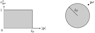
Figure 1: Zero-temperature distribution function of a free Fermi gas in the ground state (left) and with one added particle (right).

The one-to-one correspondence starts from a free Fermi gas consisting of $N$ particles, where the ground state is given by a filled Fermi sphere in momentum space, see Fig. 1. The particle number density $n$ and the ground-state energy $E_{0}$ are given by (with $\hbar=c=1$)

$$n=\frac{1}{V}\sum_{\mathbf{p}\sigma}n_{\mathbf{p}\sigma}^{0}=\frac{k_{\text{F}}^{3}}{3\pi^{2}}\quad\text{and}\quad E_{0}=\sum_{\mathbf{p}\sigma}\frac{\mathbf{p}^{2}}{2m}\,n_{\mathbf{p}\sigma}^{0}=\frac{3}{5}\frac{k_{\text{F}}^{2}}{2m}\,N\,,$$ (1)

where $k_{\text{F}}$ denotes the Fermi momentum, $V$ the volume, and $n_{\mathbf{p}\sigma}^{0}=\theta(k_{\text{F}}-|\mathbf{p}|)$ is the Fermi-Dirac distribution function at zero temperature for particles with momentum $\mathbf{p}$, spin projection $\sigma$, and mass $m$. By adding particles or holes, the distribution function is changed by $\delta n_{\mathbf{p}\sigma}=n_{\mathbf{p}\sigma}-n_{\mathbf{p}\sigma}^{0}$, and the total energy of the system by

$$\delta E=E-E_{0}=\sum_{\mathbf{p}\sigma}\frac{\mathbf{p}^{2}}{2m}\,\delta n_{\mathbf{p}\sigma}\,.$$ (2)

When a particle is added in the state $\mathbf{p}\sigma$, one has $\delta n_{\mathbf{p}\sigma}=1$ and when a particle is removed (a hole is added) $\delta n_{\mathbf{p}\sigma}=-1$.

In the interacting system the corresponding state is one with a quasiparticle added or removed, and the change in energy is given by

$$\delta E=\sum_{\mathbf{p}\sigma}\varepsilon_{\mathbf{p}\sigma}\,\delta n_{\mathbf{p}\sigma}\,,$$ (3)

where $\varepsilon_{\mathbf{p}\sigma}=\delta E/\delta n_{\mathbf{p}\sigma}$ denotes the quasiparticle energy. When two or more quasiparticles are added to the system, an additional term takes into account the interaction between the quasiparticles:

$$\delta E=\sum_{\mathbf{p}\sigma}\varepsilon^{0}_{\mathbf{p}\sigma}\,\delta n_{\mathbf{p}\sigma}+\frac{1}{2V}\sum_{\mathbf{p}_{1}\sigma_{1},\mathbf{p}_{2}\sigma_{2}}f_{\mathbf{p}_{1}\sigma_{1}\mathbf{p}_{2}\sigma_{2}}\,\delta n_{\mathbf{p}_{1}\sigma_{1}}\,\delta n_{\mathbf{p}_{2}\sigma_{2}}\,.$$ (4)

Here $\varepsilon^{0}_{\mathbf{p}\sigma}$ is the quasiparticle energy in the ground state. In the next section, we will show that the expansion in $\delta n$ is general and does not require weak interactions. The small expansion parameter in Fermi liquid theory is the density of quasiparticles, or equivalently the excitation energy, and not the strength of the interaction. This allows a systematic treatment of strongly interacting systems at low temperatures.

The second term in Eq. (4), the quasiparticle interaction $f_{\mathbf{p}_{1}\sigma_{1}\mathbf{p}_{2}\sigma_{2}}$, has no correspondence in the non-interacting Fermi gas. In an excited state with more than one quasiparticle, the quasiparticle energy is modified according to

$$\varepsilon_{\mathbf{p}\sigma}=\frac{\delta E}{\delta n_{\mathbf{p}\sigma}}=\varepsilon^{0}_{\mathbf{p}\sigma}+\frac{1}{V}\sum_{\mathbf{p}_{2}\sigma_{2}}f_{\mathbf{p}\sigma\mathbf{p}_{2}\sigma_{2}}\,\delta n_{\mathbf{p}_{2}\sigma_{2}}\,,$$ (5)

where the changes are effectively proportional to the quasiparticle density.

The quasiparticle interaction can be understood microscopically from the second variation of the energy with respect to the quasiparticle distribution,

$$f_{\mathbf{p}_{1}\sigma_{1}\mathbf{p}_{2}\sigma_{2}}=V\,\frac{\delta^{2}E}{\delta n_{\mathbf{p}_{1}\sigma_{1}}\delta n_{\mathbf{p}_{2}\sigma_{2}}}=V\,\frac{\delta\varepsilon_{\mathbf{p}_{1}\sigma_{1}}}{\delta n_{\mathbf{p}_{2}\sigma_{2}}}\,.$$ (6)

As discussed in detail in Section 2.5, this variation diagrammatically corresponds to cutting one of the fermion lines in a given energy diagram and labeling the incoming and outgoing fermion by $\mathbf{p}_{1}\sigma_{1}$, followed by a second variation leading to $\mathbf{p}_{2}\sigma_{2}$. For the uniform system, the resulting contributions to $f_{\mathbf{p}_{1}\sigma_{1}\mathbf{p}_{2}\sigma_{2}}$ are quasiparticle reducible in the particle-particle and in the exchange particle-hole (induced interaction) channels, but irreducible in the direct particle-hole (zero sound) channel. The zero-sound reducible diagrams are generated by the particle-hole scattering equation.

In normal Fermi systems, the quasiparticle concept makes sense only for states close to the Fermi surface, where the quasiparticle life-time $\tau_{\mathbf{p}}$ is long. The leading term is quadratic in the momentum difference from the Fermi surface BaymPethick , $1/\tau_{\mathbf{p}}\sim(p-k_{\text{F}})^{2}$, while the dependence of the quasiparticle energy is linear, $\varepsilon_{\mathbf{p}}-\mu\sim(p-k_{\text{F}})$. Thus, the condition

$$|\varepsilon_{\mathbf{p}}-\mu|\gg\frac{1}{\tau_{\mathbf{p}}}\,,$$ (7)

which is needed for the quasiparticle to be well defined, is satisfied by states close enough to the Fermi surface. Generally, quasiparticles are useful for time scales $\tau\ll\tau_{\mathbf{p}}$ and thus for high frequencies $|\omega|\tau_{\mathbf{p}}\gg 1$. In particular, states deep in the Fermi sea, which are occupied in the ground-state distribution, do not correspond to well-defined quasiparticles. Accordingly, we refer to the interacting ground state that corresponds to a filled Fermi sea in the non-interacting system as a state with no quasiparticles. In a weakly excited state the quasiparticle distribution $\delta n_{\mathbf{p}\sigma}$ is generally non-zero only for states close to the Fermi surface.

For low-lying excitations, the quasiparticle energy $\varepsilon_{\mathbf{p}\sigma}$ and interaction $f_{\mathbf{p}_{1}\sigma_{1}\mathbf{p}_{2}\sigma_{2}}$ is needed only for momenta close to the Fermi momentum $k_{\text{F}}$. It is then sufficient to retain the leading term in the expansion of $\varepsilon_{\mathbf{p}\sigma}-\mu$ around the Fermi surface, and to take the magnitude of the quasiparticle momenta in $f_{\mathbf{p}_{1}\sigma_{1}\mathbf{p}_{2}\sigma_{2}}$ equal to the Fermi momentum. In an isotropic and spin-saturated system ($N_{\uparrow}=N_{\downarrow}$), and if the interaction between free particles is invariant under $SU(2)$ spin symmetry (so that there are no non-central contributions, such as $\sim{\bm{\sigma}}\cdot\mathbf{p}$ to the energy), we have

$$\varepsilon_{\mathbf{p}\sigma}-\mu=\varepsilon_{p}-\mu\approx v_{\text{F}}(p-k_{\text{F}})+\ldots\,,$$ (8)

where $v_{\text{F}}=k_{\text{F}}/m^{*}$ denotes the Fermi velocity and $m^{*}$ is the effective mass. In addition, the quasiparticle interaction can be decomposed as

$$f_{\mathbf{p}_{1}\sigma_{1}\mathbf{p}_{2}\sigma_{2}}=f_{\mathbf{p}_{1}\mathbf{p}_{2}}^{s}+f^{a}_{\mathbf{p}_{1}\mathbf{p}_{2}}\>{\bm{\sigma}}_{1}\cdot{\bm{\sigma}}_{2}\,,$$ (9)

where

$$f^{s}_{\mathbf{p}_{1}\mathbf{p}_{2}}=\frac{1}{2}\,\bigl{(}f_{\mathbf{p}_{1}\uparrow\mathbf{p}_{2}\uparrow}+f_{\mathbf{p}_{1}\uparrow\mathbf{p}_{2}\downarrow}\bigr{)}\quad\text{and}\quad f^{a}_{\mathbf{p}_{1}\mathbf{p}_{2}}=\frac{1}{2}\,\bigl{(}f_{\mathbf{p}_{1}\uparrow\mathbf{p}_{2}\uparrow}-f_{\mathbf{p}_{1}\uparrow\mathbf{p}_{2}\downarrow}\bigr{)}\,.$$ (10)

In nuclear physics the notation $f_{\mathbf{p}_{1}\mathbf{p}_{2}}=f^{s}_{\mathbf{p}_{1}\mathbf{p}_{2}}$ and $g_{\mathbf{p}_{1}\mathbf{p}_{2}}=f^{a}_{\mathbf{p}_{1}\mathbf{p}_{2}}$ is generally used, and the quasiparticle interaction includes additional terms that take into account the isospin dependence and non-central tensor contributions MigdalBook ; GerryPR ; tensor . However, for our discussion here, the spin and isospin dependence is not important.

For the uniform system, Eq. (6) yields the quasiparticle interaction only for forward scattering (low momentum transfers). In the particle-hole channel, this corresponds to the long-wavelength limit. This restriction, which is consistent with considering low excitation energies, constrains the momenta $\mathbf{p}_{1}$ and $\mathbf{p}_{2}$ to be close to the Fermi surface, $|\mathbf{p}_{1}|=|\mathbf{p}_{2}|=k_{\text{F}}$. The quasiparticle interaction then depends only on the angle between $\mathbf{p}_{1}$ and $\mathbf{p}_{2}$. It is convenient to expand this dependence on Legendre polynomials

$$f_{\mathbf{p}_{1}\mathbf{p}_{2}}^{s/a}=f^{s/a}(\cos\theta_{\mathbf{p}_{1}\mathbf{p}_{2}})=\sum_{l}\,f_{l}^{s/a}\,P_{l}(\cos\theta_{\mathbf{p}_{1}\mathbf{p}_{2}})\,,$$ (11)

and to define the dimensionless Landau Parameters $F_{l}^{s/a}$ by

$$F_{l}^{s/a}=N(0)\,f_{l}^{s/a}\,,$$ (12)

where $N(0)=\frac{1}{V}\sum_{\mathbf{p}\sigma}\delta(\varepsilon_{\mathbf{p}\sigma}-\mu)=m^{*}k_{\text{F}}/\pi^{2}$ denotes the quasiparticle density of states at the Fermi surface.

The Landau parameters can be directly related to macroscopic properties of the system. $F_{1}^{s}$ determines the effective mass and the specific heat $c_{V}$,

$$\frac{m^{*}}{m} =1+\frac{F^{s}_{1}}{3}\,,$$ (13)

$$c_{V} =\frac{m^{*}k_{\text{F}}}{3}\,k_{B}^{2}T\,,$$ (14)

while the compressibility $K$ and incompressibility $\kappa$ are given by $F_{0}^{s}$,

$$K =-\frac{1}{V}\frac{\partial V}{\partial P}=\frac{1}{n^{2}}\frac{\partial n}{\partial\mu}=\frac{1}{n^{2}}\frac{N(0)}{1+F_{0}^{s}}\,,$$ (15)

$$\kappa =\frac{9}{nK}=-\frac{9V}{n}\frac{\partial P}{\partial V}=9\,\frac{\partial P}{\partial n}=\frac{3k_{\text{F}}^{2}}{m^{*}}\,(1+F_{0}^{s})\,.$$ (16)

Moreover, the spin susceptibility $\chi_{m}$ is related to $F_{0}^{a}$,

$$\chi_{m}=\frac{\partial m}{\partial H}=\beta^{2}\frac{N(0)}{1+F_{0}^{a}}\,,$$ (17)

for spin-$1/2$ fermions with magnetic moment $\beta=ge/(4m)$ and gyromagnetic ratio $g$. Finally, a stability analysis of the Fermi surface against small amplitude deformations leads to the Pomeranchuk criteria Pomeranchuk

$$F_{l}^{s/a}>-(2l+1)\,.$$ (18)

For instance $F_{0}^{s/a}<-1$ implies an instability against spontaneous growth of density/spin fluctuations.

Landau’s theory of normal Fermi liquids is an effective low-energy theory in the modern sense Shankar ; Polchinski . The effective theory incorporates the symmetries of the system and the low-energy couplings can be fixed by experiment or calculated microscopically based on the underlying theory. Fermi Liquid theory has been very successful in describing low-temperature Fermi liquids, in particular liquid ³He. Applications to the normal phase are reviewed, for example, in Baym and Pethick BaymPethick and Pines and Nozières PinesNozieres , while we refer to Wölfle and Vollhardt WoelfleVollhardt for a description of the superfluid phases. The first applications to nuclear systems were pioneered by Migdal MigdalBook and first microscopic calculations for nuclei and nuclear matter by Brown et al. GerryPR . Recently, advances using RG methods for nuclear forces Vlowk have lead to the development of a non-perturbative RG approach for nucleonic matter RGnm , to a first complete study of the spin structure of induced interactions tensor , and to new calculations of Fermi liquid parameters indint ; Kaiser .

2.2 Three-quasiparticle interactions

In Section 2.1, we introduced Fermi liquid theory as an expansion in the density of quasiparticles $\delta n/V$. In applications of Fermi liquid theory to date, even for liquid ³He, which is a very dense and strongly interacting system, this expansion is truncated after the second-order $(\delta n)^{2}$ term, including only pairwise interactions of quasiparticles (see Eq. (4)). However, for a strongly interacting system, there is a priori no reason that three-body (or higher-body) interactions between quasiparticles are small. In this section, we discuss the convergence of this expansion. Three-quasiparticle interactions arise from iterated two-body forces, leading to three- and higher-body clusters in the linked-cluster expansion, or through many-body forces. While three-body forces play an important role in nuclear physics RMP ; matter ; nuclei , little is known about them in other Fermi liquids. Nevertheless, in strongly interacting systems, the contributions of many-body clusters can in general be significant, leading to potentially important $(\delta n)^{3}$ terms in the Fermi liquid expansion, also in the absence of three-body forces:

$$\delta E=\sum_{1}\varepsilon^{0}_{1}\>\delta n_{1}+\frac{1}{2V}\sum_{1,2}f^{(2)}_{1,2}\>\delta n_{1}\,\delta n_{2}+\frac{1}{6V^{2}}\sum_{1,2,3}f^{(3)}_{1,2,3}\>\delta n_{1}\,\delta n_{2}\,\delta n_{3}\,.$$ (19)

Here $f^{(n)}_{1,\ldots,n}$ denotes the $n$-quasiparticle interaction (the Landau interaction is $f\equiv f^{(2)}$) and we have introduced the short-hand notation $n\equiv{\bf p}_{n}\sigma_{n}$.

In order to better understand the expansion, Eq. (19), around the interacting ground state with $N$ fermions, consider exciting or adding $N_{q}$ quasiparticles with $N_{q}\ll N$. The microscopic contributions from many-body clusters or from many-body forces can be grouped into diagrams containing zero, one, two, three, or more quasiparticle lines. The terms with zero quasiparticle lines contribute to the interacting ground state for $\delta n=0$, whereas the terms with one, two, and three quasiparticle lines contribute to $\varepsilon^{0}_{1}$, $f^{(2)}_{1,2}$, and $f^{(3)}_{1,2,3}$, respectively (these also depend on the ground-state density due to the $N$ fermion lines). The terms with more than three quasiparticle lines would contribute to higher-quasiparticle interactions. Because a quasiparticle line replaces a line summed over $N$ fermions when going from $\varepsilon^{0}_{1}$ to $f^{(2)}_{1,2}$, and from $f^{(2)}_{1,2}$ to $f^{(3)}_{1,2,3}$, it is intuitively clear that the contributions due to three-quasiparticle interactions are suppressed by $N_{q}/N$ compared to two-quasiparticle interactions, and that the Fermi liquid expansion is effectively an expansion in $N_{q}/N$ or $n_{q}/n$ PinesNozieres .

Fermi liquid theory applies to normal Fermi systems at low energies and temperatures, or equivalently at low quasiparticle densities. We first consider excitations that conserve the net number of quasiparticles, $\delta N=\sum_{\mathbf{p}\sigma}\delta n_{\mathbf{p}\sigma}=0$, so that the number of quasiparticles equals the number of quasiholes. This corresponds to the lowest energy excitations of normal Fermi liquids. We denote their energy scale by $\Delta$. Excitations with one valence particle or quasiparticle added start from energies of order the chemical potential $\mu$. In the case of $\delta N=0$, the contributions of two-quasiparticle interactions are of the same order as the first-order $\delta n$ term, but three-quasiparticle interactions are suppressed by $\Delta/\mu$ Chris . This is the reason that Fermi liquid theory with only two-body Landau parameters is so successful in describing even strongly interacting and dense Fermi liquids. This counting is best seen from the variation of the free energy $F=E-\mu N$,

$$\delta F =\delta(E-\mu N)$$

$$=\sum_{1}(\varepsilon^{0}_{1}-\mu)\,\delta n_{1}+\frac{1}{2V}\sum_{1,2}f^{(2)}_{1,2}\>\delta n_{1}\,\delta n_{2}+\frac{1}{6V^{2}}\sum_{1,2,3}f^{(3)}_{1,2,3}\>\delta n_{1}\,\delta n_{2}\,\delta n_{3}\,,$$ (20)

which for $\delta N=0$ is equivalent to $\delta E$ of Eq. (19). The quasiparticle distribution is $|\delta n_{\mathbf{p}\sigma}|\sim 1$ within a shell around the Fermi surface $|\varepsilon^{0}_{\mathbf{p}\sigma}-\mu|\sim\Delta$. The first-order $\delta n$ term is therefore proportional to $\Delta$ times the number of quasiparticles $\sum_{\mathbf{p}\sigma}|\delta n_{\mathbf{p}\sigma}|=N_{q}\sim N(\Delta/\mu)$, and

$$\sum_{1}(\varepsilon^{0}_{1}-\mu)\,\delta n_{1}\sim\frac{N\Delta^{2}}{\mu}\,.$$ (21)

Correspondingly, the contribution of two-quasiparticle interactions yields

$$\frac{1}{2V}\sum_{1,2}f^{(2)}_{1,2}\>\delta n_{1}\,\delta n_{2}\sim\frac{1}{V}\,\langle f^{(2)}\rangle\,\biggl{(}\frac{N\Delta}{\mu}\biggr{)}^{2}\sim\langle F^{(2)}\rangle\,\frac{N\Delta^{2}}{\mu}\,,$$ (22)

where $\langle F^{(2)}\rangle=n\,\langle f^{(2)}\rangle/\mu$ is an average dimensionless coupling on the order of the Landau parameters. Even in the strongly interacting, scale-invariant case $\langle f^{(2)}\rangle\sim 1/k_{\text{F}}$; hence $\langle F^{(2)}\rangle\sim 1$ and the contribution of two-quasiparticle interactions is of the same order as the first-order term. However, the three-quasiparticle contribution is of order

$$\frac{1}{6V^{2}}\sum_{1,2,3}f^{(3)}_{1,2,3}\>\delta n_{1}\,\delta n_{2}\,\delta n_{3}\sim\frac{n^{2}}{\mu}\,\langle f^{(3)}\rangle\,\frac{N\Delta^{3}}{\mu^{2}}\sim\langle F^{(3)}\rangle\,\frac{N\Delta^{3}}{\mu^{2}}\,.$$ (23)

Therefore at low excitation energies this is suppressed by $\Delta/\mu$, compared to two-quasiparticle interactions, even if the dimensionless three-quasiparticle interaction $\langle F^{(3)}\rangle=n^{2}\langle f^{(3)}\rangle/\mu$ is strong (of order 1). Similarly, higher $n$-body interactions are suppressed by $(\Delta/\mu)^{n-2}$. Normal Fermi systems at low energies are weakly coupled in this sense. The small parameter is the ratio of the excitation energy per particle to the chemical potential. These considerations hold for all normal Fermi systems where the underlying interparticle interactions are finite range.

The Fermi liquid expansion in $\Delta/\mu$ is equivalent to an expansion in $N_{q}/N\sim\Delta/\mu$, the ratio of the number of quasiparticles and quasiholes $N_{q}$ to the number of particles $N$ in the interacting ground state, or an expansion in the density of excited quasiparticles over the ground-state density, $n_{q}/n$. For the case where $N_{q}$ quasiparticles or valence particles are added to a Fermi-liquid ground state, $\delta N\neq 0$ and the first-order term is

$$\sum_{1}\varepsilon^{0}_{1}\>\delta n_{1}\sim\mu N_{q}\sim\mu\,\frac{N\Delta}{\mu}\sim N\Delta\,,$$ (24)

while the contribution of two-quasiparticle interactions is suppressed by $N_{q}/N\sim\Delta/\mu$ and that of three-quasiparticle interactions by $(N_{q}/N)^{2}$.

Therefore, either for $\delta N=0$ or $\delta N\neq 0$, the contributions of three-quasiparticle interactions to normal Fermi systems at low excitation energies are suppressed by the ratio of the quasiparticle density to the ground-state density, or equivalently by the ratio of the excitation energy over the chemical potential. This holds for excitations that conserve the number of particles (excited states of the interacting ground state) as well as for excitations that add or remove particles. This suppression is general and applies to strongly interacting systems even with strong, but finite-range three-body forces. However, this does not imply that the contributions from three-body forces to the interacting ground-state energy (the energy of the core nucleus in the context of shell-model calculations), to quasiparticle energies, or to two-quasiparticle interactions are small. The argument only applies to the effects of residual three-body interactions at low energies.

2.3 Microscopic foundation of Fermi liquid theory

A central object in microscopic approaches to many-body systems is the one-body (time-ordered) propagator or Green’s function $G$ defined by

$$G(1,2)=-i\,\langle 0|{\mathcal{T}}\psi(1)\psi^{\dagger}(2)|0\rangle\,,$$ (25)

where $|0\rangle$ denotes the ground state of the system, ${\mathcal{T}}$ is the time-ordering operator, $\psi$ and $\psi^{\dagger}$ annihilate and create a fermion, respectively, and 1, 2 are short hand for space, time and internal degrees of freedom (such as spin and isospin). For a translationally invariant spin-saturated system that is also invariant under rotations in spin space, the Green’s function is diagonal in spin and can be written in momentum space as

$$G(\omega,\mathbf{p})\,\delta_{\sigma_{1}\sigma_{2}}=\int d(1-2)\,G(1,2)\,e^{i\omega(t_{1}-t_{2})-i\mathbf{p}\cdot(\mathbf{x}_{1}-\mathbf{x}_{2})}=\frac{\delta_{\sigma_{1}\sigma_{2}}}{\omega-\frac{p^{2}}{2m}-\Sigma(\omega,\mathbf{p})}\,,$$ (26)

where $\Sigma(\omega,\mathbf{p})$ defines the self-energy. For an introduction to many-body theory and additional details, we refer to the books by Fetter and Walecka FW , Abrikosov, Gor’kov and Dzyaloshinski AGD , Negele and Orland NO , and Altland and Simons AS .

Figure 2: Analytic structure of the free one-body Green’s function $G_{0}$ in the complex $\omega$ plane with simple poles for $p>k_{\text{F}}$ (left) and $p<k_{\text{F}}$ (right).

Without interactions the self-energy vanishes and consequently the free Green’s function $G_{0}$ reads

$$G_{0}(\omega,\mathbf{p})=\frac{1}{\omega-\frac{p^{2}}{2m}+i\delta_{\mathbf{p}}}=\frac{1-n^{0}_{\mathbf{p}}}{\omega-\frac{p^{2}}{2m}+i\delta}+\frac{n^{0}_{\mathbf{p}}}{\omega-\frac{p^{2}}{2m}-i\delta}\,,$$ (27)

where $\delta_{\mathbf{p}}=\delta\>{\rm sign}(p-k_{\text{F}})$ and $\delta$ is a positive infinitesimal. The free Green’s function has simple poles, as illustrated in Fig. 2, and the imaginary part takes the form

$${\rm Im}\,G_{0}(\omega,\mathbf{p})=-\pi\,(1-2n^{0}_{\mathbf{p}})\,\delta\biggl{(}\omega-\frac{p^{2}}{2m}\biggr{)}\,.$$ (28)

The single-particle spectral function $\rho(\omega,\mathbf{p})$ is determined by the imaginary part of the retarded propagator

$$G^{R}(1,2) =-i\,\theta(t_{1}-t_{2})\,\langle 0|\bigl{\{}\psi(1),\psi^{\dagger}(2)\bigr{\}}|0\rangle\,,$$ (29)

$$\rho(\omega,\mathbf{p}) =-\frac{1}{\pi}\,{\rm Im}\,G^{R}(\omega,\mathbf{p})\,,$$ (30)

where $\{\>,\>\}$ denotes the anticommutator. The retarded propagator is analytic in the upper complex $\omega$ plane and fulfills Kramers-Kronig relations, which relate the real and imaginary parts. Physically this implies that all modes are propagating forward in time and causality is fulfilled. Therefore, response functions are usually expressed in terms of the retarded propagator.

In a non-interacting system the retarded propagator is given by

$$G_{0}^{R}(\omega,\mathbf{p}) =\frac{1}{\omega-\frac{p^{2}}{2m}+i\delta}\,,$$ (31)

$${\rm Im}\,G_{0}^{R}(\omega,\mathbf{p}) =-\pi\,\delta\biggl{(}\omega-\frac{p^{2}}{2m}\biggr{)}\,,$$ (32)

which implies that the free spectral function is a delta function $\rho_{0}(\omega,\mathbf{p})=\delta(\omega-\frac{p^{2}}{2m})$. This simple form follows from the fact that single-particle plane-wave states are eigenstates of the non-interacting Hamiltonian.

In the interacting case the situation is more complicated. Here the quasiparticle energy is given implicitly by the Dyson equation

$$\varepsilon_{\mathbf{p}}=\frac{p^{2}}{2m}+\Sigma(\varepsilon_{\mathbf{p}},\mathbf{p})\,.$$ (33)

At the chemical potential $\omega=\mu$, the imaginary part of the self-energy vanishes,

$${\rm Im}\,\Sigma(\mu,\mathbf{p})=0\,,$$ (34)

and the quasiparticle life-time $\tau_{\mathbf{p}}\to\infty$ for $|\mathbf{p}|\to k_{\text{F}}$. For $\omega\neq\mu$, the imaginary part of the self-energy obeys

$${\rm Im}\,\Sigma(\omega,\mathbf{p}) <0\,\text{, for }\omega>\mu\,,$$ (35)

$${\rm Im}\,\Sigma(\omega,\mathbf{p}) >0\,\text{, for }\omega<\mu\,.$$ (36)

The retarded self-energy, which enters the retarded Green’s function

$$G^{R}(\omega,\mathbf{p})=\frac{1}{\omega-\frac{p^{2}}{2m}-\Sigma^{R}(\omega,\mathbf{p})}\,,$$ (37)

is related to the time-ordered one through

$${\rm Re}\,\Sigma^{R}(\omega,\mathbf{p}) ={\rm Re}\,\Sigma(\omega,\mathbf{p})\,,$$ (38)

$${\rm Im}\,\Sigma^{R}(\omega,\mathbf{p}) =\biggl{\{}\begin{array}[]{l}+{\rm Im}\,\Sigma(\omega,\mathbf{p})<0\,\text{, for }\omega>\mu\,,\\[2.84526pt] -{\rm Im}\,\Sigma(\omega,\mathbf{p})<0\,\text{, for }\omega<\mu\,.\end{array}$$ (41)

Using Eq. (30), one finds the general form of the spectral function

$$\rho(\omega,\mathbf{p})=-\frac{1}{\pi}\frac{{\rm Im}\,\Sigma^{R}(\omega,\mathbf{p})}{\bigl{[}\omega-\frac{p^{2}}{2m}-{\rm Re}\,\Sigma^{R}(\omega,\mathbf{p})\bigr{]}^{2}+\bigl{[}{\rm Im}\,\Sigma^{R}(\omega,\mathbf{p})\bigr{]}^{2}}\,.$$ (42)

In the interacting case the single-particle strength is therefore, for a given momentum state, fragmented in energy, and the spectral function provides a measure of the single-particle strength in the eigenstates of the Hamiltonian, with the normalization $\int_{-\infty}^{\infty}d\omega\,\rho(\omega,\mathbf{p})=1$.

The spectral or Källén-Lehmann representation of the Green’s function,

$$G^{R}(\omega,\mathbf{p})=\int_{-\infty}^{\infty}d\omega^{\prime}\>\frac{\rho(\omega^{\prime},\mathbf{p})}{\omega-\omega^{\prime}+i\delta}\,,$$ (43)

follows from analyticity and implies that the full propagator is completely determined by the spectral function. Using Eq. (43) and the normalization condition, the asymptotic ($|\omega|\rightarrow\infty$) behavior of both $G^{R}(\omega,\mathbf{p})$ and $G(\omega,\mathbf{p})\sim 1/\omega$ follows. Furthermore, the singularities of the full Green’s function (that correspond to eigenvalues of the Hamiltonian) are all located on the real axis and result in a cut along the real axis in the continuum limit. The quasiparticle pole, on the other hand, is located off the real axis, on an unphysical Riemann sheet, with the distance to the real axis given by the quasiparticle width,

$$\text{quasiparticle pole $(p\gtrsim k_{\text{F}})$: }\>\omega_{\mathbf{p}}^{\rm qp} =\varepsilon_{\mathbf{p}}-i\Gamma_{\mathbf{p}}\,,$$

$$\text{quasihole pole $(p\lesssim k_{\text{F}})$: }\>\omega_{\mathbf{p}}^{\rm qp} =\varepsilon_{\mathbf{p}}+i\Gamma_{\mathbf{p}}\,.$$ (46)

A pole close to the real axis gives rise to a peak in the single-particle strength, as illustrated in Fig. 3. Hence, microscopically a quasiparticle or quasihole is identified by a well-defined peak in the spectral function. In other words, the excitation of a quasiparticle corresponds to the coherent excitation of several eigenstates $H|\psi_{i}\rangle=E_{i}|\psi_{i}\rangle$ of the Hamiltonian, with similar energies $E_{i}$ ($\omega^{\prime}\approx\varepsilon_{\mathbf{p}}$ in Eq. (43)) spread over the quasiparticle width $\Gamma_{\mathbf{p}}=\tau_{\mathbf{p}}^{-1}$. A quasiparticle created at $t=0$ then propagates in time as

$$|\psi_{\rm qp}(t)\rangle=\sum_{i}\,c_{i}\,e^{-iE_{i}t}\,|\psi_{i}\rangle\,.$$ (47)

For short times, $t\ll 1/\Gamma_{\mathbf{p}}$, the eigenstates remain coherent and the quasiparticle is well defined, while for $t\gg 1/\Gamma_{\mathbf{p}}$, the phase coherence is lost and the quasiparticle decays.

Figure 3: Spectral function $\rho(\omega,\mathbf{p})$ for a given momentum $p\gtrsim k_{\text{F}}$ as a function of frequency $\omega$. The shaded part marks the quasiparticle peak, with quasiparticle width $\Gamma_{\mathbf{p}}$ and single-particle strength $z_{\mathbf{p}}$.

Using this definition of a quasiparticle, the full propagator can be formally separated into a quasiparticle part and a smooth background $\phi(\omega,\mathbf{p})$:

$$G(\omega,\mathbf{p})=\frac{z_{\mathbf{p}}}{\omega-\varepsilon_{\mathbf{p}}+i\Gamma_{\mathbf{p}}}+\phi(\omega,\mathbf{p})\,,$$ (48)

where the single-particle strength $z_{\mathbf{p}}$ carried by the quasiparticle is given by

$$z_{\mathbf{p}}=\biggl{[}1-\frac{\partial\Sigma(\omega,\mathbf{p})}{\partial\omega}\biggr{|}_{\omega=\varepsilon_{\mathbf{p}}}\biggr{]}^{-1}<1\,,$$ (49)

and must be less than unity due to the normalization of the spectral function.

Close to the Fermi surface the width $\Gamma_{\mathbf{p}}$ is small, $\Gamma_{\mathbf{p}}\sim(p-k_{\text{F}})^{2}$, and consequently quasiparticles are well defined. For processes with a typical time scale $\tau<\tau_{\mathbf{p}}=\Gamma_{\mathbf{p}}^{-1}$, the contribution of the quasiparticle remains coherent, while that of the smooth background is incoherent. Even for very small values of the single-particle strength $z_{\mathbf{p}}$, quasiparticles play a leading role at sufficiently low excitation energies.

2.4 Scattering of quasiparticles

Figure 4: Scattering channels in a many-fermion system. The direct particle-hole or zero-sound (ZS) channel (left), the exchange particle-hole (ZS^′) channel (middle) and the particle-particle/hole-hole (BCS) channel (right). The relative incoming and outgoing four-momenta $k,k^{\prime}$ are related to the momentum transfers $q,q^{\prime}$ by $k=(q^{\prime}+q)/2$ and $k^{\prime}=(q^{\prime}-q)/2$. The center-of-mass momentum is denoted by $P$.

Quasiparticle scattering processes are in general described by the Bethe-Salpeter equation. The quasiparticle scattering amplitude is given by the full four-point function $\Gamma$, which includes contributions from scattering in the channels shown in Fig. 4. For small $q=(\omega,\mathbf{q})$, the contribution of the direct particle-hole or zero-sound (ZS) channel is singular due to a pinching of the integration contour by the quasiparticle poles of the two intermediate propagators for any external momenta $p_{1}=(P+q^{\prime})/2$ and $p_{2}=(P-q^{\prime})/2$, as discussed below and in detail in Ref. AGD . In contrast, for small $q$ the exchange particle-hole (ZS^′) and the particle-particle/hole-hole (BCS) channels are smooth for almost all external momenta.

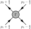
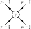
$\quad=\quad$ $\quad+\quad$

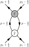
Figure 5: The Bethe-Salpeter equation in the ZS channel, Eq. (50).

The Bethe-Salpeter equation that sums all ZS-channel reducible diagrams is shown diagrammatically in Fig. 5 and reads

$$\Gamma(p_{1},p_{2};q)=\widetilde{\Gamma}(p_{1},p_{2};q)\\ -i\int\frac{d^{4}p}{(2\pi)^{4}}\,\widetilde{\Gamma}(p_{1},p;q)\,G(p+q/2)\,G(p-q/2)\,\Gamma(p,p_{2};q)\,,$$ (50)

where $\widetilde{\Gamma}$ denotes the ZS-channel irreducible four-point function and we suppress the spin of the fermions for simplicity. The singular part of the two intermediate propagators is obtained by using the quasiparticle representation of the Green’s function, Eq. (48), and for $q\to 0$ one finds

$$G(p+q/2)\,G(p-q/2)=\frac{z_{\mathbf{p}+\mathbf{q}/2}}{\varepsilon+\omega/2-\mu-v_{\text{F}}(|\mathbf{p}+\mathbf{q}|/2-k_{\text{F}})+i\delta_{|\mathbf{p}+\mathbf{q}|/2}}$$

$$\times\frac{z_{\mathbf{p}-\mathbf{q}/2}}{\varepsilon-\omega/2-\mu-v_{\text{F}}(|\mathbf{p}-\mathbf{q}|/2-k_{\text{F}})+i\delta_{|\mathbf{p}-\mathbf{q}|/2}}+\phi_{2}(p)\,,$$

$$=2\pi i\,z_{k_{\text{F}}}^{2}\,\frac{|\mathbf{q}|\cos\theta_{\mathbf{p}\mathbf{q}}}{\omega-v_{\text{F}}|\mathbf{q}|\cos\theta_{\mathbf{p}\mathbf{q}}}\,\delta(\varepsilon-\mu)\,\delta(|\mathbf{p}|-k_{\text{F}})+\phi_{2}(p)\,,$$ (51)

where $p=(\varepsilon,\mathbf{p})$. The first term in Eq. (51) is the quasiparticle-quasihole part, which constrains the intermediate states to the Fermi surface, and the contribution $\phi_{2}(p)$ includes at least one power of the smooth background $\phi(p)$. In addition, we have taken $q\to 0$ in all nonsingular terms and neglected the quasiparticle width, which is small close to the Fermi surface.

We observe that the quasiparticle-quasihole part of the particle-hole propagator vanishes in the limit $|\mathbf{q}|/\omega\to 0$. Therefore, we define

$$\Gamma^{\omega}(p_{1},p_{2}) =\underset{\omega\rightarrow 0}{{\rm lim}}\bigl{(}\Gamma(p_{1},p_{2};q)\bigr{|}_{|\mathbf{q}|=0}\bigr{)}\,,$$ (52)

$$\Gamma^{q}(p_{1},p_{2}) =\underset{|\mathbf{q}|\rightarrow 0}{{\rm lim}}\bigl{(}\Gamma(p_{1},p_{2};q)\bigr{|}_{\omega=0}\bigr{)}\,.$$ (53)

Using the quasiparticle-quasihole representation of the particle-hole propagator, Eq. (51), the Bethe-Salpeter equation in the ZS channel takes the form

$$\Gamma(p_{1},p_{2};q)=\widetilde{\Gamma}(p_{1},p_{2};q)-i\int\frac{d^{4}p}{(2\pi)^{4}}\,\widetilde{\Gamma}(p_{1},p;q)\,\phi_{2}(p)\,\Gamma(p,p_{2};q)\\ +\frac{z_{k_{\text{F}}}^{2}k_{\text{F}}^{2}}{(2\pi)^{3}}\int d\Omega_{\mathbf{p}}\,\widetilde{\Gamma}(p_{1},p;q)\,\frac{|\mathbf{q}|\cos\theta_{\mathbf{p}\mathbf{q}}}{\omega-v_{\text{F}}|\mathbf{q}|\cos\theta_{\mathbf{p}\mathbf{q}}}\,\Gamma(p,p_{2};q)\,.$$ (54)

In the limit $|\mathbf{q}|/\omega\to 0$, we have for the quasiparticle-quasihole irreducible part of the four-point function $\Gamma^{\omega}$,

$$\Gamma^{\omega}(p_{1},p_{2})=\widetilde{\Gamma}(p_{1},p_{2})-i\int\frac{d^{4}p}{(2\pi)^{4}}\,\widetilde{\Gamma}(p_{1},p)\,\phi_{2}(p)\,\Gamma^{\omega}(p,p_{2})\,.$$ (55)

Using $\Gamma^{\omega}$, we can then eliminate the ZS-channel irreducible four-point function $\widetilde{\Gamma}$ and the background term $\phi_{2}$ to write the Bethe-Salpeter equation in the form

$$\Gamma(p_{1},p_{2};q)=\Gamma^{\omega}(p_{1},p_{2})+\frac{z_{k_{\text{F}}}^{2}k_{\text{F}}^{2}}{(2\pi)^{3}}\int d\Omega_{\mathbf{p}}\Gamma^{\omega}(p_{1},p)\frac{|\mathbf{q}|\cos\theta_{\mathbf{p}\mathbf{q}}}{\omega-v_{\text{F}}|\mathbf{q}|\cos\theta_{\mathbf{p}\mathbf{q}}}\Gamma(p,p_{2};q).$$ (56)

In the limit $\omega/|\mathbf{q}|\to 0$ one then finds

$$\Gamma^{q}(p_{1},p_{2})=\Gamma^{\omega}(p_{1},p_{2})-\frac{z_{k_{\text{F}}}^{2}m^{*}k_{\text{F}}}{(2\pi)^{3}}\int d\Omega_{\mathbf{p}}\,\Gamma^{\omega}(p_{1},p)\,\Gamma^{q}(p,p_{2})\,,$$ (57)

which describes the scattering of quasiparticles. By identifying the quasiparticle interaction with (as justified in Section 2.5)

$$f_{\mathbf{p}_{1}\mathbf{p}_{2}}=z_{k_{\text{F}}}^{2}\,\Gamma^{\omega}(p_{1},p_{2})\bigr{|}_{\omega_{1}=\varepsilon_{\mathbf{p}_{1}},\,\omega_{2}=\varepsilon_{\mathbf{p}_{2}}}\,,$$ (58)

and the quasiparticle scattering amplitude with

$$a_{\mathbf{p}_{1}\mathbf{p}_{2}}=z_{k_{\text{F}}}^{2}\,\Gamma^{q}(p_{1},p_{2})\bigr{|}_{\omega_{1}=\varepsilon_{\mathbf{p}_{1}},\,\omega_{2}=\varepsilon_{\mathbf{p}_{2}}}\,,$$ (59)

the Bethe-Salpeter equation for the quasiparticle scattering amplitude reads

$$a_{\mathbf{p}_{1}\sigma_{1}\mathbf{p}_{2}\sigma_{2}}=f_{\mathbf{p}_{1}\sigma_{1}\mathbf{p}_{2}\sigma_{2}}-\frac{N(0)}{8\pi}\,\sum_{\sigma}\int d\Omega_{\mathbf{p}}\,a_{\mathbf{p}_{1}\sigma_{1}\mathbf{p}\sigma}\,f_{\mathbf{p}\sigma\mathbf{p}_{2}\sigma_{2}}\,,$$ (60)

where we have reintroduced spin indices. By expanding the angular dependence of the quasiparticle scattering amplitude on Legendre polynomials,

$$a_{\mathbf{p}_{1}\mathbf{p}_{2}}^{s/a}=a^{s/a}(\cos\theta_{\mathbf{p}_{1}\mathbf{p}_{2}})=\sum_{l}\,a_{l}^{s/a}\,P_{l}(\cos\theta_{\mathbf{p}_{1}\mathbf{p}_{2}})\,,$$ (61)

and using the corresponding expansion of the quasiparticle interaction, Eq. (11), the quasiparticle scattering equation, Eq. (60), can be solved analytically for each value of $l$,

$$A_{l}^{s,a}=\cfrac{F_{l}^{s,a}}{1+\cfrac{F_{l}^{s,a}}{2l+1}}\,,$$ (62)

with $A_{l}^{s,a}=N(0)\,a_{l}^{s,a}$. This analytic solution of the quasiparticle scattering equation, Eq. (56), is in general possible only in the limit $q\to 0$.

Quasiparticles are fermionic excitations and therefore obey the Pauli principle. This imposes nontrivial constraints on the Landau parameters, as can be seen by the following argument. The full four-point function must be antisymmetric under exchange of two particles in the initial or final states,

$$\parbox{88.2037pt}{\includegraphics[scale={0.82},clip={}]{Pauli1.eps}}=\hskip 5.69054pt-\hskip 11.38109pt\parbox{88.2037pt}{\includegraphics[scale={0.82},clip={}]{Pauli2.eps}}\,,$$ (63)

and therefore the forward scattering amplitude, $q=0$, of identical particles, $q^{\prime}=0$ and $\sigma_{1}=\sigma_{2}$, must vanish. This implies $a_{\mathbf{p}_{1}\sigma_{1}\mathbf{p}_{1}\sigma_{1}}=0$, which leads to the Pauli-principle sum rule Landau3 ; AK

$$\sum_{l}\,\bigl{(}A_{l}^{s}+A_{l}^{a}\bigr{)}=0\,.$$ (64)

The relations given in this section can be generalized to include isospin and tensor forces GerryPR ; tensor ; BSJ ; FD , which play an important role in nuclear systems.

2.5 Functional approach

Functional methods provide a powerful tool for studying many-body systems. We start by discussing the two-particle irreducible (2PI) effective action. This provides a useful framework for an RG approach to many-body systems. For simplicity, we first consider bosonic systems described by a scalar field $\phi$ and generalize the results later to fermions. Our discussion follows Ref. CJT . We start with the expression for the generating functional $W$ for connected $N$-point functions

$$W[J,K]=-\ln\int\mathcal{D}\phi\,\exp\biggl{[}iS[\phi]-\int d^{4}x\,\phi(x)\,J(x)\\ -\frac{1}{2}\int d^{4}x\,d^{4}y\,\phi(x)\,K(x,y)\,\phi(y)\biggr{]}\,,$$ (65)

where $\int\mathcal{D}\phi$ denotes a functional integral over the field $\phi$, the action is given by $S[\phi]=\int d^{4}x\,\mathcal{L}(\phi(x))$, and $J(x)$ and $K(x,y)$ are external sources. In thermodynamic equilibrium, the space-time integral is

$$\int d^{4}x=\int_{0}^{-i\beta}dt\int d^{3}x\,,$$ (66)

with inverse temperature $\beta=1/T$. By taking functional derivatives with respect to $J$ and $K$, we obtain the expectation value of the field $\overline{\phi}=\langle\phi\rangle$ and the Green’s function $G$ respectively,

$$\frac{\delta W[J,K]}{\delta J(x)} =\langle\phi(x)\rangle=\overline{\phi}(x)\,,$$ (67)

$$\frac{\delta W[J,K]}{\delta K(x,y)} =\frac{1}{2}\Bigl{(}\overline{\phi}(x)\overline{\phi}(y)+G(x,y)\Bigr{)}\,.$$ (68)

A double Legendre transform leads to the 2PI effective action $\Gamma[\overline{\phi},G]$,

$$\Gamma[\overline{\phi},G]=W[J,K]-\int d^{4}x\,\overline{\phi}(x)\,J(x)\\ -\frac{1}{2}\int d^{4}x\ d^{4}y\,\Bigl{[}\overline{\phi}(x)\,\overline{\phi}(y)+G(x,y)\Bigr{]}K(x,y)\,,$$ (69)

which is stationary with respect to variations of $\overline{\phi}$ and $G$ for vanishing sources,

$$\frac{\delta\Gamma[\overline{\phi},G]}{\delta\overline{\phi}(x)} =-J(x)-\int d^{4}y\,K(x,y)\,\overline{\phi}(y)\overset{J=K=0}{=}0\,,$$ (70)

$$\frac{\delta\Gamma[\overline{\phi},G]}{\delta G(x,y)} =-\frac{1}{2}\,K(x,y)\overset{J=K=0}{=}0\,.$$ (71)

An explicit form for $\Gamma$ in terms of the expectation value $\overline{\phi}$ and the exact Green’s function $G$ can be constructed following Refs. CJT ; LW ; Baym . This leads to

$$\Gamma[\overline{\phi},G]=-iS[\overline{\phi}]+{\rm Tr}\ln G^{-1}+{\rm Tr}\Bigr{[}(G_{0}^{-1}-G^{-1})G\Bigr{]}-\Phi[\overline{\phi},G]\,.$$ (72)

Here the functional $\Phi$ is the sum of all 2PI skeleton diagrams (for a discussion of diagrams, see below) and the trace is a short-hand notation for

$${\rm Tr}=\int d^{4}x\>{\rm tr}=\int_{0}^{-i\beta}dt\int d^{3}x\>{\rm tr}\,,$$ (73)

where ${\rm tr}$ denotes the trace over the internal degrees of freedom, such as spin and isospin. The stationarity of the 2PI effective action in the absence of sources, Eqs. (70) and (71), leads to the gap and Dyson equations, respectively. With the explicit form for $\Gamma$, Eq. (72), the Dyson equation is given by

$$\frac{\delta\Gamma[\overline{\phi},G]}{\delta G}=-G^{-1}+G_{0}^{-1}+\frac{\delta\Phi[\overline{\phi},G]}{\delta G}=0\,,$$ (74)

which implies

$$G^{-1}=G_{0}^{-1}-\Sigma\,,$$ (75)

with the self-consistently determined self-energy $\Sigma$ defined by

$$\Sigma=\frac{\delta\Phi[\overline{\phi},G]}{\delta G}\,.$$ (76)

At the stationary point, the 2PI effective action $\Gamma$ is proportional to the thermodynamic potential $\Omega=T\Gamma$ (in units with volume $V=1$) Wetterich :

$$\Omega(\mu,T)=-\int d^{3}x\,\mathcal{L}(\overline{\phi}(x))+\Omega_{0}(\mu,T)+T\,\Bigl{[}{\rm Tr}\ln(1-G_{0}\Sigma)+{\rm Tr}\Sigma G-\Phi(\overline{\phi},G)\Bigr{]}\,,$$ (77)

where we have introduced the thermodynamic potential of the non-interacting Bose gas,

$$\Omega_{0}(\mu,T)=T\,{\rm Tr}\ln G_{0}^{-1}=T\,{\rm tr}\int\frac{d{\bf p}}{(2\pi)^{3}}\,\ln\biggl{[}1-\exp\Bigl{[}-\beta\,\Bigl{(}\frac{{\bf p}^{2}}{2m}-\mu\Bigr{)}\Bigr{]}\biggr{]}\,,$$ (78)

and the third term on the right-hand side of Eq. (77) can also be written as $-T\,{\rm Tr}\ln G_{0}^{-1}+T\,{\rm Tr}\ln G^{-1}$, so that $\Omega_{0}(\mu,T)+T\,{\rm Tr}\ln(1-G_{0}\Sigma)=T\,{\rm Tr}\ln G^{-1}$. Finally, one can verify that the form of the 2PI effective action given by Eq. (77), where the self-energy enters explicitly, is stationary with respect to independent variations of $G$ and $\Sigma$.

Similarly one has for the thermodynamic potential of a system consisting of fermions (where the expectation value $\langle\psi\rangle$ vanishes in the absence of sources)

$$\Omega(\mu,T)=-T\,\Bigl{[}{\rm Tr}\ln G^{-1}+{\rm Tr}\Sigma G-\Phi[G]\Bigr{]}\,.$$ (79)

Moreover the energy of a fermionic system can be expressed at $T=0$ in a form similar to Eq. (77),

$$E=E_{0}-{\rm Tr}\ln(1-G_{0}\Sigma)-{\rm Tr}\Sigma G+\Phi[G]\,.$$ (80)

Here $E_{0}={\rm tr}\int\frac{d{\bf p}}{(2\pi)^{3}}\,\frac{{\bf p}^{2}}{2m}\,n^{0}_{{\bf p}\sigma}$ is the energy of the non-interacting system, and at $T=0$ the trace in Eq. (80) is given by

$${\rm Tr}={\rm tr}\int\frac{d^{4}p}{(2\pi)^{4}i}={\rm tr}\oint_{\mathcal{C}}\frac{d\omega}{2\pi i}\,\frac{d{\bf p}}{(2\pi)^{3}}\,,$$ (81)

where the integration contour $\mathcal{C}$ is shown in Fig. 6.

Figure 6: Integration contour in the complex $\omega$ plane at $T=0$.

Next, we use the functional integral approach to relate the quasiparticle interaction to the quasiparticle-quasihole irreducible part of the four-point function $\Gamma^{\omega}$ following Ref. Nozieres . In the quasiparticle approximation, the full propagator takes the form of Eq. (48),

$$G(\omega,\mathbf{p})=\frac{1}{G_{0}^{-1}(\omega,\mathbf{p})-\Sigma(\omega,\mathbf{p})}=\frac{z_{\mathbf{p}}}{\omega-\varepsilon_{\mathbf{p}}+i\delta_{\mathbf{p}}}+\phi(\omega,\mathbf{p})\,,$$ (82)

where we have neglected the imaginary part of the self-energy for excitations close to the Fermi surface. As shown in Section 2.3, the quasiparticle energy $\varepsilon_{\mathbf{p}}$ is given by the self-consistent solution to the Dyson equation, Eq. (33),

$$\varepsilon_{\mathbf{p}}=\frac{\mathbf{p}^{2}}{2m}+\Sigma(\varepsilon_{\mathbf{p}},\mathbf{p})\,,$$ (83)

and the single-particle strength $z_{\mathbf{p}}$ by Eq. (49). When a quasiparticle with momentum $\mathbf{p}$ is added to the system, the state is changed from unoccupied to occupied, so that $\delta_{\mathbf{p}}=\delta\rightarrow-\delta$, with positive infinitesimal $\delta>0$. Because the 2PI effective action is stationary with respect to independent variations of $G$ and $\Sigma$, we only need to consider changes of $E_{0}$ and those induced by variations of $G_{0}$ in Eq. (80). In the quasiparticle approximation, we have for the argument of the logarithm,

$$1-G_{0}(p)\Sigma(p)=G_{0}(p)\,G^{-1}(p)=\frac{1}{z_{\mathbf{p}}}\,\frac{\omega-\varepsilon_{\mathbf{p}}+i\delta_{\mathbf{p}}}{\omega-\frac{\mathbf{p}^{2}}{2m}+i\delta_{\mathbf{p}}}+\text{smooth parts.}$$ (84)

Consider the case $\varepsilon_{\mathbf{p}}>\frac{\mathbf{p}^{2}}{2m}$. Then the real part of $G_{0}\,G^{-1}$ is negative for $\frac{\mathbf{p}^{2}}{2m}<\omega<\varepsilon_{\mathbf{p}}$, resulting in a cut on the real energy, as shown in Fig. 7. When a particle is added to the system, the integration contour changes from above the cut to below, and $\ln(G_{0}\,G^{-1})$ changes by $-2\pi i$ for $\frac{\mathbf{p}^{2}}{2m}<\omega<\varepsilon_{\mathbf{p}}$. As a result, the change in the energy of the system is given by

$$\frac{\delta E}{\delta n_{\mathbf{p}}} =\frac{\delta E_{0}}{\delta n_{\mathbf{p}}}-\frac{\delta}{\delta n_{\mathbf{p}}}\biggl{(}\,\oint_{\mathcal{C}}\frac{d\omega}{2\pi i}\,\frac{d{\bf p}}{(2\pi)^{3}}\,\ln\bigl{(}G_{0}(p)\,G^{-1}(p)\bigr{)}\biggr{)}\,,$$ (85)

$$=\frac{\mathbf{p}^{2}}{2m}+\biggl{(}\varepsilon_{\mathbf{p}}-\frac{\mathbf{p}^{2}}{2m}\,\biggr{)}=\varepsilon_{\mathbf{p}}\,.$$ (86)

This variation is the quasiparticle energy, as postulated by Landau.

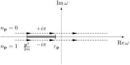
Figure 7: Analytic structure of $\ln(G_{0}\,G^{-1})$ in the complex $\omega$ plane for $\varepsilon_{\mathbf{p}}>\frac{\mathbf{p}^{2}}{2m}$. The upper (lower) contour is for $n_{\bf p}=0$ ($n_{\bf p}=1$) and the shaded region represents the complex cut on the real axis.

As discussed in Section 2.1, the quasiparticle interaction $f_{\mathbf{p}_{1}\mathbf{p}_{2}}$ is obtained by an additional variation with respect to the occupation number $n_{\mathbf{p}_{2}}$,

$$f_{\mathbf{p}_{1}\mathbf{p}_{2}}=\frac{\delta^{2}E}{\delta n_{\mathbf{p}_{1}}\,\delta n_{\mathbf{p}_{2}}}=\frac{\delta\varepsilon_{\mathbf{p}_{1}}}{\delta n_{\mathbf{p}_{2}}}\,.$$ (87)

Using the Dyson equation, Eq. (83), the variation of the quasiparticle energy $\varepsilon_{\mathbf{p}_{1}}$ with respect to the occupation number $n_{\mathbf{p}_{2}}$ yields

$$\frac{\delta\varepsilon_{\mathbf{p}_{1}}}{\delta n_{\mathbf{p}_{2}}}=\frac{\delta\Sigma(\omega_{1},\mathbf{p}_{1})}{\delta n_{\mathbf{p}_{2}}}\biggr{|}_{\omega_{1}=\varepsilon_{\mathbf{p}_{1}}}+\frac{\partial\Sigma(\omega_{1},\mathbf{p}_{1})}{\partial\omega_{1}}\biggr{|}_{\omega_{1}=\varepsilon_{\mathbf{p}_{1}}}\frac{\delta\varepsilon_{\mathbf{p}_{1}}}{\delta n_{\mathbf{p}_{2}}}\,.$$ (88)

This can be expressed with the single-particle strength $z_{\mathbf{p}}$ as

$$\frac{\delta\varepsilon_{\mathbf{p}_{1}}}{\delta n_{\mathbf{p}_{2}}}=z_{\mathbf{p}_{1}}\,\frac{\delta\Sigma(\omega_{1},\mathbf{p}_{1})}{\delta n_{\mathbf{p}_{2}}}\biggr{|}_{\omega_{1}=\varepsilon_{\mathbf{p}_{1}}}\,.$$ (89)

Furthermore, it follows from the definition of $\Sigma$ through the $\Phi$ functional, $\Sigma(p)=\delta\Phi[G]/\delta G(p)$, that the self-energy consists of skeleton diagrams. Therefore, we can write

$$\frac{\delta\Sigma(\omega_{1},\mathbf{p}_{1})}{\delta n_{\mathbf{p}_{2}}}\biggr{|}_{\omega_{1}=\varepsilon_{\mathbf{p}_{1}}}=\int\frac{d^{4}p}{(2\pi)^{4}i}\>\frac{\delta\Sigma(\omega_{1},\mathbf{p}_{1})}{\delta G(p)}\,\frac{\delta G(p)}{\delta n_{\mathbf{p}_{2}}}\biggr{|}_{\omega_{1}=\varepsilon_{\mathbf{p}_{1}}}\,.$$ (90)

The variation of $\Sigma$ with respect to $G$ selects one of the internal lines of the diagrams contributing to the self-energy. As a result, the kernel

$$\widetilde{\Gamma}(p_{1},p_{2})=\frac{\delta\Sigma(p_{1})}{\delta G(p_{2})}\,,$$ (91)

must be particle-hole irreducible in the ZS channel. Otherwise the corresponding diagram in $\Sigma$ would not have been a 2PI skeleton diagram. This is illustrated in Fig. 8.

Figure 8: Only 2PI skeleton diagrams contribute to the self-energy $\Sigma$, as shown on the left. Non-skeleton diagrams, such as the one on the right, are not part of $\Sigma$. Therefore, the kernel $\widetilde{\Gamma}=\delta\Sigma/\delta G$ (denoted by the shaded blob) is particle-hole irreducible in the ZS channel.

Using the quasiparticle form of the full propagator, Eq. (82), there are two contributions to $\delta G(p_{1})/\delta n_{\mathbf{p}_{2}}$ (for details, see also Ref. Nozieres ). One for $p_{1}=p_{2}$ ($\omega_{2}=\varepsilon_{\mathbf{p}_{2}}$), which results in a shift of the quasiparticle pole across the integration contour, and one for $p_{1}\neq p_{2}$, which corresponds to a variation of the self-energy,

$$\frac{\delta G(p_{1})}{\delta n_{\mathbf{p}_{2}}}=(2\pi)^{4}i\,z_{\mathbf{p}_{2}}\,\delta(\mathbf{p}_{1}-\mathbf{p}_{2})\delta(\omega_{1}-\varepsilon_{\mathbf{p}_{2}})+\frac{\delta\Sigma(p_{1})}{\delta n_{\mathbf{p}_{2}}}\,G^{2}(p_{1})\,.$$ (92)

The $G^{2}(p_{1})$ part in the second term is equivalent to the non-singular contribution $\phi_{2}(p_{1})$ of Eq. (51). By inserting this expression for $\delta G(p_{1})/\delta n_{\mathbf{p}_{2}}$ in Eq. (90), one finds the integral equation

$$Y(p_{1},p_{2}) =\frac{1}{z_{\mathbf{p}_{2}}}\frac{\delta\Sigma(\omega_{1},\mathbf{p}_{1})}{\delta n_{\mathbf{p}_{2}}}\biggr{|}_{\omega_{1}=\varepsilon_{\mathbf{p}_{1}}}\,$$ (93)

$$=\widetilde{\Gamma}(p_{1},p_{2})+\int\frac{d^{4}p}{(2\pi)^{4}i}\>\widetilde{\Gamma}(p_{1},p)\,G^{2}(p)\,Y(p,p_{2})\,.$$ (94)

A comparison with Eq. (55) leads to the identification

$$Y(p_{1},p_{2})=\Gamma^{\omega}(p_{1},p_{2})=\frac{1}{z_{\mathbf{p}_{2}}}\frac{\delta\Sigma(\omega_{1},\mathbf{p}_{1})}{\delta n_{\mathbf{p}_{2}}}\biggr{|}_{\omega_{1}=\varepsilon_{\mathbf{p}_{1}}}\,.$$ (95)

Using Eq. (89), this implies

$$f_{\mathbf{p}_{1}\mathbf{p}_{2}}=\frac{\delta\varepsilon_{\mathbf{p}_{1}}}{\delta n_{\mathbf{p}_{2}}}=z_{\mathbf{p_{1}}}z_{\mathbf{p}_{2}}\,\Gamma^{\omega}(p_{1},p_{2})=\parbox{76.82234pt}{\includegraphics[scale={0.82},clip={}]{Gamma_z.eps}}\,.$$ (96)

This provides a microscopic basis for calculating the quasiparticle energy $\varepsilon_{\mathbf{p}}=\frac{\delta E}{\delta n_{\mathbf{p}_{1}}}$ and the quasiparticle interaction $f_{\mathbf{p}_{1}\mathbf{p}_{2}}=\frac{\delta^{2}E}{\delta n_{\mathbf{p}_{1}}\delta n_{\mathbf{p}_{2}}}$ and a justification for the identification of the quasiparticle interaction as in Eq. (58).

$E^{(2)}$	$\varepsilon^{(2)}_{\mathbf{p}}$	$f^{(2)}_{\mathbf{p}_{1}\mathbf{p}_{2}}$

Figure 9: The variation of the second-order energy diagram $E^{(2)}$ (left) with respect to the quasiparticle distribution function yields the second-order contribution to the quasiparticle energy $\varepsilon^{(2)}_{\mathbf{p}}$ given by the self-energy diagram (middle) and the corresponding two-hole–one-particle diagram. The second variation gives the second-order contributions to the quasiparticle interaction (right). These include the particle-particle and particle-hole diagrams shown and a particle-hole diagram that is obtained from the particle-particle one by reversing the arrow on the $p_{2}$ line (plus the diagrams obtained from the two-hole–one-particle self-energy contribution).

The contributions to the quasiparticle interaction can be understood by considering the variation of the second-order energy diagram, as shown in Fig. 9. The resulting diagrams in $f_{\mathbf{p}_{1}\mathbf{p}_{2}}$ are quasiparticle-quasihole reducible in the BCS and ZS^′ channels, but irreducible in the ZS channel (see Fig. 4 for a definition of the BCS, ZS and ZS^′ channels). The ZS reducible diagrams, which are shown for the second-order example in Fig. 10, are included in the scattering amplitude $a_{\mathbf{p}_{1}\mathbf{p}_{2}}$ but not in the quasiparticle interaction. Because the ZS and ZS^′ channels are related by exchange BB , the quasiparticle scattering amplitude is antisymmetric, but the quasiparticle interaction is not.

Figure 10: Second-order diagrams that are not generated by variations of the energy diagram.

$\quad=\quad$ $\quad+\quad$

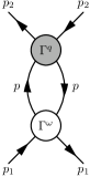
Figure 11: The Bethe-Salpeter equation for the quasiparticle scattering amplitude, Eq. (57), which sums diagrams reducible in the ZS channel. The intermediate-state propagators include only the quasiparticle-quasihole part. All other contributions are included in $\Gamma^{\omega}$.

The quasiparticle-quasihole reducible diagrams in the ZS channel are summed by the Bethe-Salpeter equation, Eq. (57), which yields the fully reducible four-point function $\Gamma^{q}$, given the quasiparticle-quasihole irreducible one $\Gamma^{\omega}$, as shown in Fig. 11. The fully reducible four-point function $\Gamma^{q}$ corresponds to the quasiparticle scattering amplitude. The four-point function can also be obtained by summing diagrams that are quasiparticle-quasihole reducible in the ZS^′ channel. The corresponding Bethe-Salpeter equation is shown in Fig. 12, where the irreducible term is the quasiparticle interaction in the ZS^′ channel, the exchange of $\Gamma^{\omega}$ denoted by $\overline{\Gamma^{\omega}}$.

$\quad=\quad$ $\quad+\quad$

Figure 12: The Bethe-Salpeter equation for the quasiparticle scattering amplitude in the exchange (ZS^′) channel. In this channel, the solution requires as input the quasiparticle scattering amplitude $\Gamma^{q}$ and the quasiparticle interaction $\Gamma^{\omega}$ at finite $q$. As in Fig. 11, the intermediate-state propagators include only the quasiparticle-quasihole part.

$\quad=\quad$ $\quad+\quad$

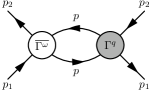
Figure 13: Integral equation for the quasiparticle interaction $\Gamma^{\omega}$ that sums quasiparticle-quasihole reducible diagrams in the ZS^′ channel. The second term on the right hand side is the induced interaction of Babu and Brown BB .

The kinematics in the integral term on the right-hand side of Fig. 12 requires as input the quasiparticle scattering amplitude $\Gamma^{q}$ and the quasiparticle interaction $\Gamma^{\omega}$ at finite $q$. Therefore, we can generalize $\Gamma^{q}$ on the left-hand side to finite $q$. If we then take the limit $|\mathbf{q}|/\omega\to 0$, all quasiparticle-quasihole reducible terms in the ZS channel vanish. In this limit, $\Gamma^{q}$ on the left-hand side of Fig. 12 is replaced by $\Gamma^{\omega}$, and the first term on the right hand side, $\overline{\Gamma^{\omega}}$, is reduced to the driving term $I$, which is quasiparticle-quasihole irreducible in both ZS and ZS^′ channels. As a result, we obtain an integral equation for $\Gamma^{\omega}$ that sums quasiparticle-quasihole reducible diagrams in the ZS^′ channel. This is shown diagrammatically in Fig. 13, where the second term on the right hand side is the induced interaction of Babu and Brown BB (see also Ref. indint ). For $p_{1}=p_{2}$, this integral equation has the simple form,

$$\Gamma^{\omega}(p_{1},p_{1})=I(p_{1},p_{1})-P_{\bm{\sigma}}\,\frac{z_{k_{\text{F}}}^{2}m^{*}k_{\text{F}}}{(2\pi)^{3}}\,\sum\limits_{\sigma}\int d\Omega_{\mathbf{p}}\,\Gamma^{\omega}(p_{1},p)\,\Gamma^{q}(p,p_{1})\,.$$ (97)

The induced interaction accounts for the contributions to the quasiparticle interaction due to the polarization of the medium and is necessary for the antisymmetry of the quasiparticle scattering amplitude $\Gamma^{q}$.

3 Functional RG approach to Fermi liquid theory

In this section we apply the functional RG Wetterich93 to calculate the properties of a Fermi liquid. The basic idea is to renormalize the quasiparticle energy and the quasiparticle interaction, as one sequentially integrates out the excitations of the system. Thereby, one starts with the high-lying states and integrates down to low excitation energy. The functional RG leads to an infinite set of coupled differential equations for the $n$-point functions, which in practical calculations must be truncated. We return to this question below, when we discuss applications.

In zero-temperature Fermi systems, the low-lying states are those near the Fermi surface. Consequently, at some intermediate step of the calculation, the high-lying states, far above and far below the Fermi surface have been integrated out, while the states near the Fermi surface are not yet included. This is schematically illustrated in Fig. 14. However, in the first part of this section we keep the discussion more general and allow for finite temperatures. In the second part, we apply the RG approach to a Fermi liquid at zero temperature and also specify the detailed form of the regulator adapted to Fermi systems at zero temperature.

Figure 14: The cutoffs above and below the Fermi surface separate high- and low-lying excitations of the many-fermion system.

The Green’s function

$$G_{\Lambda 0}^{-1}(\omega,\mathbf{p})=\omega-\frac{\mathbf{p}^{2}}{2m}-R_{\Lambda}(\mathbf{p})\,,$$ (98)

with regulator $R_{\Lambda}(\mathbf{p})$ defines the free theory at a finite cutoff scale $\Lambda$. The corresponding effective action is given by (see Eq. (72) and the corresponding expression for fermions, Eq. (79))

$$\Gamma_{\Lambda}(\psi^{\ast},\psi,G)=-iS_{\Lambda}(\psi^{\ast},\psi)-\text{Tr}\ln(-G^{-1})-\text{Tr}[G_{\Lambda 0}^{-1}G-1]+\Phi(\psi^{\ast},\psi,G)\,,$$ (99)

with the action

$$S_{\Lambda}(\psi^{\ast},\psi)=-i\,T\sum_{n}\int\frac{d^{3}p}{(2\pi)^{3}}\,\psi^{*}(\omega_{n},\mathbf{p})\biggl{(}\omega_{n}-\frac{\mathbf{p}^{2}}{2m}-R_{\Lambda}(\mathbf{p})\biggr{)}\psi(\omega_{n},\mathbf{p})\,,$$ (100)

and Matsubara frequency $\omega_{n}=(2n+1)i\pi T$. At the stationary point, the propagator $G$ satisfies the Dyson equation (see Eqs. (75) and (76))

$$G_{\Lambda}^{-1}=G_{\Lambda 0}^{-1}-\frac{\delta\Phi(\psi^{\ast},\psi,G)}{\delta G}\biggr{|}_{G=G_{\Lambda}}\,,$$ (101)

and therefore acquires a dependence on $\Lambda$. Due to the stationarity of the 2PI effective action with respect to variations of $\psi$, $\psi^{\ast}$, and $G$, only the explicit $\Lambda$ dependence of the bare Green’s function $G_{\Lambda 0}$ contributes to the flow equation for the effective action:

$$\frac{d\Gamma_{\Lambda}(\psi^{\ast},\psi,G_{\Lambda})}{d\Lambda} = \text{Tr}\biggl{[}\frac{\delta\Gamma_{\Lambda}(\psi^{\ast},\psi,G_{\Lambda})}{\delta G^{-1}_{\Lambda 0}(p)}\frac{dG^{-1}_{\Lambda 0}(p)}{d\Lambda}\biggr{]}$$ (102)

$$= \text{Tr}\biggl{[}\psi^{*}_{p}\,\frac{dR_{\Lambda}(\mathbf{p})}{d\Lambda}\,\psi_{p}\biggr{]}+\text{Tr}\biggl{[}G_{\Lambda}(p)\,\frac{dR_{\Lambda}(\mathbf{p})}{d\Lambda}\biggr{]}\,,$$

where we have introduced the short-hand notations $\psi_{p}=\psi(\omega_{n},\mathbf{p})$ and ${\rm{Tr}}=T\,\sum_{n}\int\frac{d\mathbf{p}}{(2\pi)^{3}}$. The flow equation follows almost trivially from the stationarity of the 2PI effective action, while within a 1PI scheme, the derivation of the flow equation is somewhat more involved Wetterich93 ; BTW . The flow equation for the two-point function in the 1PI scheme is obtained by varying Eq. (102) with respect to $\psi$ and $\psi^{\ast}$. Using

$$\Gamma^{\Lambda(2)}_{p,p}=\frac{\delta^{2}\Gamma_{\Lambda}}{\delta\psi^{\ast}_{p}\,\delta\psi_{p}}=G_{\Lambda}^{-1}(p)\,,$$ (103)

and

$$\frac{\delta^{2}G_{\Lambda}(p^{\prime})}{\delta\psi^{\ast}_{p}\,\delta\psi_{p}}=-G_{\Lambda}(p^{\prime})\,\Gamma^{\Lambda(4)}_{p,p,p^{\prime},p^{\prime}}\,G_{\Lambda}(p^{\prime})\quad\text{with}\quad\Gamma^{\Lambda(4)}_{p,p,p^{\prime},p^{\prime}}=\frac{\delta^{2}\Gamma^{\Lambda(2)}_{p,p}}{\delta\psi^{\ast}_{p^{\prime}}\,\delta\psi_{p^{\prime}}}\,,$$ (104)

one finds

$$\frac{d\Gamma^{\Lambda(2)}_{p,p}}{d\Lambda}=-\frac{dR_{\Lambda}(\mathbf{p})}{d\Lambda}-\text{Tr}\biggl{[}\Gamma^{\Lambda(4)}_{p,p,p^{\prime},p^{\prime}}\,G_{\Lambda}(p^{\prime})\,\frac{dR_{\Lambda}(\mathbf{p}^{\prime})}{d\Lambda}\,G_{\Lambda}(p^{\prime})\biggr{]}\,.$$ (105)

Next, we briefly discuss the flow equation in the 2PI scheme and make a connection between the two schemes for the two-point function. Here we follow the discussion of Dupuis Dupuis . The starting point is the observation that the 2PI functional $\Phi$ does not flow, when $\psi$ and $G$ are treated as free variables

$$\frac{d\Phi(\psi,G)}{d\Lambda}\biggr{|}_{\psi,G}=0\,.$$ (106)

As discussed in the previous section, the functional $\Phi(\psi,G)$ generates the particle-hole irreducible $n$-point functions through variations with respect to the Green’s function (see also Ref. Baym )

$$\Phi^{\Lambda(2n)}_{p_{1},p_{2},\ldots,p_{2n-1},p_{2n}}=\frac{\delta^{n}\Phi(\psi,G)}{\delta G(p_{1},p_{2})\cdots\,\delta G(p_{2n-1},p_{2n})}\,.$$ (107)

After the variation, the Green’s functions satisfy the Dyson equation, Eq. (101). Consequently, the flow of the 2PI vertices $\Phi^{(n)}$ results only from the $\Lambda$ dependence of the Green’s function:

$$\frac{d}{d\Lambda}\,\Phi^{\Lambda(2n)}_{p_{1},p_{2},\ldots,p_{2n-1},p_{2n}}=\text{Tr}\biggl{[}\Phi^{\Lambda(2n+2)}_{p_{1},p_{2},\ldots,p_{2n-1},p_{2n},q,q}\,\frac{dG_{\Lambda}(q)}{d\Lambda}\biggr{]}\,.$$ (108)

Combined with the self-energy $\Sigma(p)=\Phi^{\Lambda(2)}_{p,p}$, so that $\Gamma^{\Lambda(2)}_{p,p}=G_{\Lambda 0}^{-1}(p)-\Phi^{\Lambda(2)}_{p,p}$ and $\frac{d\Gamma^{\Lambda(2)}_{p,p}}{d\Lambda}=-\frac{dR_{\Lambda}(\mathbf{p})}{d\Lambda}-\frac{d\Phi^{\Lambda(2)}_{p,p}}{d\Lambda}$, one finds

$$\frac{d\Gamma^{\Lambda(2)}_{p,p}}{d\Lambda}=-\frac{dR_{\Lambda}(\mathbf{p})}{d\Lambda}+\text{Tr}\biggl{[}\Phi^{\Lambda(4)}_{p,p,p^{\prime},p^{\prime}}\,G_{\Lambda}(p^{\prime})\,\frac{d\Gamma^{\Lambda(2)}_{p^{\prime},p^{\prime}}}{d\Lambda}\,G_{\Lambda}(p^{\prime})\biggr{]}\,.$$ (109)

The flow equations for the two-point function in the 1PI and 2PI schemes, Eqs. (105) and (109), are equivalent, as can be shown in a straightforward calculation, making use of the Bethe-Salpeter equation for scattering of two particles of vanishing total momentum Hebeler ,

$$\Gamma^{\Lambda(4)}_{p_{1},p_{1},p_{2},p_{2}}=\Phi^{\Lambda(4)}_{p_{1},p_{1},p_{2},p_{2}}+\text{Tr}\biggl{[}\Phi^{\Lambda(4)}_{p_{1},p_{1},p^{\prime},p^{\prime}}\,G_{\Lambda}(p^{\prime})\,G_{\Lambda}(p^{\prime})\,\Gamma^{\Lambda(4)}_{p^{\prime},p^{\prime},p_{2},p_{2}}\biggr{]}\,.$$ (110)

The relation between the two schemes is illustrated diagrammatically in Fig. 15. The particle-hole reducible diagrams can be shifted between the four-point function and the regulator insertion on the fermion line. For more details on the relation between the RG approaches based on 1PI and 2PI functionals the reader is referred to Ref. Dupuis .

$-$     $=$     $=$  

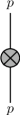
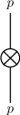
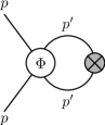
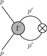
Figure 15: Graphical representation of the 1PI and 2PI flow equations for the two-point function, Eqs. (105) and (109). The internal lines represent full propagators $G_{\Lambda}$. The filled crossed circles represent $\frac{d\Gamma^{\Lambda(2)}}{d\Lambda}$ and the unfilled ones $\frac{dG_{\Lambda 0}^{-1}}{d\Lambda}=-\frac{dR_{\Lambda}}{d\Lambda}$.

We are now in a position to connect with Fermi liquid theory, by deriving a flow equation for the quasiparticle energy closely related to 1PI equation, Eq. (105). To this end, we first define the energy functional following Eq. (80)

$$E_{\Lambda}(G)=E_{\Lambda 0}-\text{Tr}\ln(G_{\Lambda 0}\,G^{-1})-\text{Tr}\bigl{[}(G_{\Lambda 0}^{-1}-G^{-1})\,G\bigr{]}+\Phi(G)\,,$$ (111)

which at the stationary point equals the (zero-temperature) ground-state energy at the cutoff scale $\Lambda$. The trace Tr is defined as in Eq. (81), $E_{\Lambda 0}$ is the energy of the non-interacting system at the scale $\Lambda$,

$$E_{\Lambda 0}=\text{tr}\int\frac{d^{3}p}{(2\pi)^{3}}\biggl{[}\frac{\mathbf{p}^{2}}{2m}+R_{\Lambda}(\mathbf{p})\biggr{]}n_{\mathbf{p},\Lambda}^{0}\,,$$ (112)

with $n_{\mathbf{p},\Lambda}^{0}=\theta(k_{\text{F}}-\Lambda-p)$, and the free Green’s function $G_{\Lambda 0}$ is given by

$$G_{\Lambda 0}(\omega,\mathbf{p})=\frac{1-n_{\mathbf{p},\Lambda}^{0}}{\omega-\frac{\mathbf{p}^{2}}{2m}-R_{\Lambda}(\mathbf{p})+i\delta}+\frac{n_{\mathbf{p},\Lambda}^{0}}{\omega-\frac{\mathbf{p}^{2}}{2m}-R_{\Lambda}(\mathbf{p})-i\delta}\,.$$ (113)

Furthermore, in the quasiparticle approximation the one-particle Green’s function of the interacting system is of the form

$$G_{\Lambda}(\omega,\mathbf{p})=z_{\mathbf{p}}\biggl{[}\frac{1-n_{\mathbf{p},\Lambda}^{0}}{\omega-\tilde{\varepsilon}_{\mathbf{p}}+i\delta}+\frac{n_{\mathbf{p},\Lambda}^{0}}{\omega-\tilde{\varepsilon}_{\mathbf{p}}-i\delta}\biggr{]}+\phi(\mathbf{p},\omega)\,,$$ (114)

where the quasiparticle energy $\tilde{\varepsilon}_{\mathbf{p}}$ is given by

$$\tilde{\varepsilon}_{\mathbf{p}}=\frac{\mathbf{p}^{2}}{2m}+\Sigma_{\Lambda}(\tilde{\varepsilon}_{\mathbf{p}},{\mathbf{p}})+R_{\Lambda}(\mathbf{p})\,.$$ (115)

The flow equation that follows from the energy functional, Eq. (111), reads

$$\frac{dE_{\Lambda}}{d\Lambda}=\frac{dE_{\Lambda 0}}{d\Lambda}-\text{Tr}\biggl{[}(G_{\Lambda 0}-G_{\Lambda})\,\frac{dR_{\Lambda}}{d\Lambda}\biggr{]}=\text{Tr}\biggl{[}G_{\Lambda}\,\frac{dR_{\Lambda}}{d\Lambda}\biggr{]}\,.$$ (116)

By varying Eq. (116) with respect to the quasiparticle occupation number, we obtain a flow equation for the quasiparticle energy

$$\frac{d\tilde{\varepsilon}_{\mathbf{p}}}{d\Lambda} = \frac{\delta}{\delta n_{\mathbf{p}}}\frac{dE_{\Lambda}}{d\Lambda}=\frac{\delta}{\delta n_{\mathbf{p}}}\biggl{(}\text{tr}\int\frac{d^{4}p^{\prime}}{(2\pi)^{4}i}\,G_{\Lambda}(p^{\prime})\,\frac{dR_{\Lambda}(\mathbf{p}^{\prime})}{d\Lambda}\biggr{)}$$ (117)

$$= z_{\mathbf{p}}\,\frac{dR_{\Lambda}(\mathbf{p})}{d\Lambda}+\text{tr}\int\frac{d^{4}p^{\prime}}{(2\pi)^{4}i}\,\frac{1}{z_{\mathbf{p^{\prime}}}}\,f_{\mathbf{p}\mathbf{p}^{\prime}}\,G_{\Lambda}^{2}(p^{\prime})\,\frac{dR_{\Lambda}(\mathbf{p}^{\prime})}{d\Lambda}\,,$$

where we have used Eqs. (92), (95) and (96). Combined with Eq. (115), the right-hand side of the flow equation for the quasiparticle energy, Eq. (117), can be written as

$$\frac{d\tilde{\varepsilon}_{\mathbf{p}}}{d\Lambda}=z_{\mathbf{p}}\biggl{(}\frac{\partial\Sigma_{\Lambda}(\tilde{\varepsilon}_{\mathbf{p}},{\mathbf{p}})}{\partial\Lambda}+\frac{dR_{\Lambda}(\mathbf{p})}{d\Lambda}\biggr{)}\equiv\frac{d\varepsilon_{\mathbf{p}}}{d\Lambda}+z_{\mathbf{p}}\,\frac{dR_{\Lambda}(\mathbf{p})}{d\Lambda}\,,$$ (118)

where we have identified ${d\varepsilon_{\mathbf{p}}}/{d\Lambda}$ with $z_{\mathbf{p}}\,{\partial\Sigma_{\Lambda}(\tilde{\varepsilon}_{\mathbf{p}},{\mathbf{p}})}/\partial\Lambda$. In the limit $\Lambda\to 0$, $\varepsilon_{\mathbf{p}}$ approaches the solution of the Dyson equation, Eq. (83).

For our purpose, we use following regulator (adapted from Ref. Morris )

$$R_{\Lambda}(\mathbf{p})=\frac{\mathbf{p}^{2}}{2m}\biggl{[}\frac{1}{\Theta_{\epsilon}(|\mathbf{p}|-(k_{\text{F}}+\Lambda))+\Theta_{\epsilon}(k_{\text{F}}-\Lambda-|\mathbf{p}|)}-1\biggr{]}\,,$$ (119)

where $\underset{\epsilon\rightarrow 0}{\text{lim}}\,\Theta_{\epsilon}(x)\rightarrow\Theta(x)$ at the end of the calculation. The regulator suppresses low-lying single-particle modes with momenta in the range $k_{F}-\Lambda<|\mathbf{p}|<k_{F}+\Lambda$ (see Fig. 14). In the limit of a sharp cutoff, $\epsilon\rightarrow 0$, one finds Morris

$$G^{2}_{\Lambda}(p)\,\frac{dR_{\Lambda}(\mathbf{p})}{d\Lambda}=-\frac{\delta(|\mathbf{p}|-(k_{\text{F}}+\Lambda))+\delta(|\mathbf{p}|-(k_{\text{F}}-\Lambda))}{\omega-\frac{\mathbf{p}^{2}}{2m}-\Sigma_{\Lambda}(\omega,\mathbf{p})}\,.$$ (120)

Keeping only the quasiparticle contribution in the second term of Eq. (117) and canceling the trivial renormalization due to the explicit regulator term in $\tilde{\varepsilon}_{\mathbf{p}}$, we find

$$\frac{d\varepsilon_{\mathbf{p}}}{d\Lambda}=-\text{tr}\int\frac{d^{3}p^{\prime}}{(2\pi)^{3}}\,f_{\mathbf{p}\mathbf{p}^{\prime}}\,n_{\mathbf{p}^{\prime},\Lambda}^{0}\Bigl{[}\delta(|\mathbf{p}^{\prime}|-(k_{\text{F}}+\Lambda))+\delta(|\mathbf{p}^{\prime}|-(k_{\text{F}}-\Lambda))\Bigr{]}\,.$$ (121)

This flow equation for the quasiparticle energy, Eq. (121), is illustrated diagrammatically in Fig. 16.

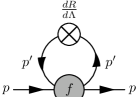
Figure 16: Flow equation for the self-energy in the quasiparticle approximation.

The four-point vertex that enters the flow equation for the self-energy is the quasiparticle-quasihole irreducible quasiparticle interaction $f_{\mathbf{p}\mathbf{p}^{\prime}}$. This result can be understood by recognizing that the quasiparticle-quasihole reducible contributions of the full four-point vertex $\Gamma^{\Lambda(4)}_{p,p,p^{\prime},p^{\prime}}$ in Eq. (105) do not contribute for the kinematics relevant to the self-energy, for $|\mathbf{q}|/\omega=0$. We can therefore replace the full four-point vertex in Eq. (105) by $\Gamma^{\omega}$, which for quasiparticle kinematics is proportional to $f_{\mathbf{p}\mathbf{p}^{\prime}}$.

The flow equation for the four-point function,

$$\Gamma^{(4)}_{p_{1}^{\prime},p_{2}^{\prime},p_{1},p_{2}}=\frac{\delta^{4}\Gamma}{\delta\psi^{\ast}_{p_{2}^{\prime}}\,\delta\psi^{\ast}_{p_{1}^{\prime}}\delta\psi_{p_{2}}\,\delta\,\psi_{p_{1}}}\,,$$ (122)

is obtained by functionally differentiating Eq. (102) twice with respect to $\psi^{\ast}$ and twice with respect to $\psi$. For details we refer the reader to Ref. Ellwanger . The resulting flow equation is illustrated diagrammatically in Fig. 17. There are two types of contributions to the flow equation: those involving two four-point functions (where all three channels, the particle-hole ZS and ZS^′ channels, as well as the particle-particle/hole-hole BCS channel contribute) and one obtained by closing two legs of the six-point function.

$\>=\>$ $\>+\>$

$\>+\>$   $\>+\>$

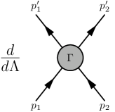
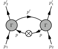
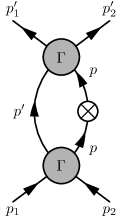
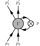
Figure 17: Flow equation for the four-point function $\Gamma^{(4)}$. For each of the first three diagrams on the right-hand side, there is an additional diagram, where the unfilled crossed circle is inserted on the other internal line.

The particle-hole channels take into account contributions to the quasiparticle scattering amplitude and interaction due to long-range density and spin-density excitations, whereas the BCS channel builds up contributions from the coupling to high-momentum states and due to pairing correlations. For the application to neutron matter, we start the many-body calculation from low-momentum interactions $V_{{\rm low}\,k}$ Vlowk , for which the particle-particle channel is perturbative at nuclear densities, except for low-lying pairing correlations matter ; Weinberg . This is in contrast to hard potentials, where the coupling to high momenta renders all channels non-perturbative.

We therefore solve the flow equations for the four-point function shown in Fig. 17 including only the particle-hole contributions (the first and second diagrams). After the RG flow, we calculate the low-lying pairing correlations by solving the quasiparticle BCS gap equation. In our first study RGnm , we neglected the contribution from the six-point function to the flow equation (the last term in Fig. 17) and approximated the internal Green’s functions by the quasiparticle part (the first term on the right-hand-side of Eq. (114)). The resulting flow equations for the quasiparticle scattering amplitude

$$a(\mathbf{q},\mathbf{q}^{\prime};\Lambda)=z_{k_{\text{F}}}^{2}\,\Gamma^{(4)}_{p-\frac{q}{2},p^{\prime}+\frac{q}{2},p+\frac{q}{2},p^{\prime}-\frac{q}{2}}\Bigl{|}_{\omega=\omega^{\prime}=\varepsilon_{\rm F},\,q_{0}=0}\,,$$ (123)

and the quasiparticle interaction $f(\mathbf{q},\mathbf{q}^{\prime};\Lambda)$ are given by RGnm :

$$\frac{d}{d\Lambda}a(\mathbf{q},\mathbf{q}^{\prime};\Lambda) = z_{k_{\text{F}}}^{2}\frac{d}{d\Lambda}\left[g\int_{\text{fast},\Lambda}\frac{d^{3}\mathbf{p}^{\prime\prime}}{(2\pi)^{3}}\frac{n_{\mathbf{p}^{\prime\prime}+\mathbf{q}/2}-n_{\mathbf{p}^{\prime\prime}-\mathbf{q}/2}}{\varepsilon_{\mathbf{p}^{\prime\prime}+\mathbf{q}/2}-\varepsilon_{\mathbf{p}^{\prime\prime}-\mathbf{q}/2}}\right]$$

$$\times a\Big{(}\mathbf{q},\frac{\mathbf{p}+\mathbf{p}^{\prime}}{2}+\frac{\mathbf{q}^{\prime}}{2}-\mathbf{p}^{\prime\prime};\Lambda\Big{)}a\big{(}\mathbf{q},\mathbf{p}^{\prime\prime}-\frac{\mathbf{p}+\mathbf{p}^{\prime}}{2}+\frac{\mathbf{q}^{\prime}}{2};\Lambda\big{)}$$

$$+ \frac{d}{d\Lambda}f(\mathbf{q},\mathbf{q}^{\prime};\Lambda)\,,$$

$$\frac{d}{d\Lambda}f(\mathbf{q},\mathbf{q}^{\prime};\Lambda) = -z_{k_{\text{F}}}^{2}\frac{d}{d\Lambda}\left[g\int_{\text{fast},\Lambda}\frac{d^{3}\mathbf{p}^{\prime\prime}}{(2\pi)^{3}}\frac{n_{\mathbf{p}^{\prime\prime}+\mathbf{q}^{\prime}/2}-n_{\mathbf{p}^{\prime\prime}-\mathbf{q}^{\prime}/2}}{\varepsilon_{\mathbf{p}^{\prime\prime}+\mathbf{q}^{\prime}/2}-\varepsilon_{\mathbf{p}^{\prime\prime}-\mathbf{q}^{\prime}/2}}\right]$$

$$\times a\big{(}\mathbf{q}^{\prime},\frac{\mathbf{p}+\mathbf{p}^{\prime}}{2}+\frac{\mathbf{q}}{2}-\mathbf{p}^{\prime\prime};\Lambda\big{)}a\big{(}\mathbf{q}^{\prime},\mathbf{p}^{\prime\prime}-\frac{\mathbf{p}+\mathbf{p}^{\prime}}{2}+\frac{\mathbf{q}}{2};\Lambda\big{)}\,.$$

Here the spin labels and the spin trace in the flow equation have been suppressed. In a spin-saturated system the spin dependence of $f$ and $a$ is of the form of Eq. (9), when non-central forces are neglected. We note that for $\mathbf{q}=\mathbf{q}^{\prime}=0$ and identical spins the contributions from the ZS and ZS^′ channels to the scattering amplitude $a$ cancel, as required by the Pauli principle. Thus, the resulting quasiparticle interaction and the corresponding Fermi liquid parameters satisfy the Pauli-principle sum rules, see Eq. (64). Moreover, the flow equations, Eqs. (3) and (3), yield the correct quasiparticle-quasihole reducibility of the scattering amplitude $a(\mathbf{q},\mathbf{q}^{\prime};\Lambda)$ and of the quasiparticle interaction $f(\mathbf{q},\mathbf{q}^{\prime};\Lambda)$.

At an initial scale $\Lambda=\Lambda_{0}$, the quasiparticle scattering amplitude and interaction start from the free-space interaction. In neutron matter, non-central and three-nucleon forces are weaker, and we therefore solved the flow equations starting from low-momentum two-nucleon (NN) interactions $V_{{\rm low}\,k}$ Vlowk ,

$$a(\mathbf{q},\mathbf{q^{\prime}};\Lambda_{0})=f(\mathbf{q},\mathbf{q^{\prime}};\Lambda_{0})=V_{\text{low}\,k}(\mathbf{q},\mathbf{q}^{\prime})\,,$$ (126)

including only scalar and spin-spin interactions, which dominate at densities below nuclear saturation density.

         

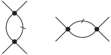
Figure 18: The free-space two-body interaction, shown by the left diagram, is the lowest order contribution to the quasiparticle scattering amplitude. The two one-loop particle-hole diagrams on the right are generated by the RG flow in the first iteration. There are two more diagrams, where the slash is on the other internal line.

It is instructive to study the RG method diagrammatically, to understand how many-body correlations are generated by the flow equations. We discuss the set of diagrams, which is generated by the flow equation for the scattering amplitude, Eq. (3). We denote the antisymmetrized free-space two-body interaction $\Gamma_{\text{vac}}$, the initial condition for the flow equation, by a dot (see Fig. 18). Starting from $\Gamma_{\text{vac}}$, we integrate out the first shell $\delta\Lambda$ of high-lying particle-hole excitations to obtain the effective scattering amplitude at the lower scale $\Lambda_{1}=\Lambda_{0}-\delta\Lambda$. The RG flow includes contributions from both particle-hole channels, which leads to the four diagrams, two of which are shown in Fig. 18. The lines marked by a slash are restricted by the regulator to momenta in the shell $\Lambda_{1}\leqslant k<\Lambda_{0}$.

 

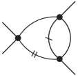
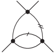
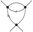
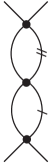
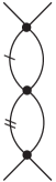
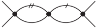
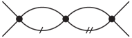
Figure 19: Two-loop diagrams that contribute to the scattering amplitude after two iterations of the flow equations.

The four-point vertex used in each iteration of the flow equation is the one obtained in the previous iteration. Thus, in the second iteration, one finds the one-loop diagrams shown in Fig. 18, but now with the momentum of the marked line in the second shell $\Lambda_{2}=\Lambda_{1}-\delta\Lambda\leqslant k<\Lambda_{1}$. In addition, the RG flow generates the two-loop diagrams shown in Fig. 19. Here, lines with momenta in the first shell are marked by one slash and those with momenta in the second shell by two slashes. For every diagram shown, there are three more diagrams obtained by moving the slash or the two slashes from a particle (hole) line to the corresponding hole (particle) line. The first four diagrams illustrate the coupling between the two particle-hole channels generated by the RG equations.

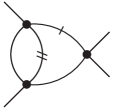
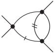
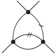
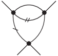
Figure 20: The two-loop planar diagrams that are not generated by the RG flow after two iterations.

We observe that the four diagrams of third order in the vacuum interaction shown in Fig. 20 are missing in this scheme. These diagrams are obtained when the last term in Fig. 17 (the contribution of the six-point function to the flow of the four-point function) is included. This shows that the flow equations reproduce the full one-loop particle-hole phase space exactly, augmented by a large antisymmetric subset of the particle-hole parquet diagrams. In a truncation scheme where the BCS channel and the six-point function in Fig. 17 is included, the RG sums all planar diagrams using the RG.

3.1 Fermi liquid parameters and scattering amplitude

In Fig. 21, we show the resulting $l=0$ and $l=1$ Fermi liquid parameters as a function of the Fermi momentum $k_{\text{F}}$. In this section we use the notation common in nuclear physics,

$$f_{\mathbf{p}\sigma\mathbf{p^{\prime}}\sigma^{\prime}} = f_{\mathbf{p}\mathbf{p}^{\prime}}+g_{\mathbf{p}\mathbf{p}^{\prime}}\,\boldsymbol{\sigma}\cdot\boldsymbol{\sigma}^{\prime}\,,$$ (127)

$$a_{\mathbf{p}\sigma\mathbf{p^{\prime}}\sigma^{\prime}} = a_{\mathbf{p}\mathbf{p}^{\prime}}+b_{\mathbf{p}\mathbf{p}^{\prime}}\,\boldsymbol{\sigma}\cdot\boldsymbol{\sigma}^{\prime}\,,$$ (128)

with $F_{l}=N_{0}\,f_{l}$ and $G_{l}=N_{0}\,g_{l}$. The cutoff scale of the starting $V_{{\rm low}\,k}$ is taken as $\Lambda=\sqrt{2}\,k_{\text{F}}$. This choice has the advantage that scattering to high-lying states in the particle-particle channel is uniformly accounted for at different densities. The low-momentum interaction $V_{{\rm low}\,k}$ then drives the flow in the ZS^′ channel for the quasiparticle interaction, and thus our results include effects of the induced interaction. A further advantage of the RG approach is that the calculations can be performed without truncating the expansion of the quasiparticle interaction, Eq. (11), at some $l$.

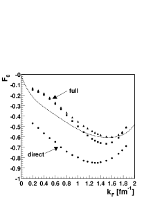
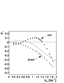
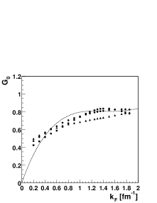
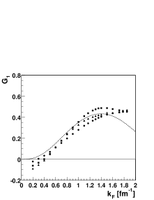
Figure 21: The $l=0$ and $l=1$ Fermi liquid parameters versus the Fermi momentum $k_{\text{F}}$. The dots denote the direct contribution only ($z_{k_{\text{F}}}$=1, but including the effective mass in the density of states), whereas the squares (static $z_{k_{\text{F}}}$ factor) and the triangles (adaptive $z_{k_{\text{F}}}$ factor) are calculated from the full RG solution. The results of Wambach et al. WAP2 are given for comparison as dashed lines.

The flow equations were solved with two different assumptions for the $z_{k_{\text{F}}}$ factor. In one case, we use a static, density-independent mean value of $z_{k_{F}}^{2}=0.9$ which remains unchanged under the RG. In the other case, we compute the $z_{k_{\text{F}}}$ factor dynamically, by assuming that the change of the effective mass from the initial one, based on the momentum dependence of $V_{{\rm low}\,k}$, is due to the $z_{k_{\text{F}}}$ factor alone RGnm . Generally, we find a very good agreement between our results and the ones obtained using the polarization potential model by Ainsworth et al. WAP1 ; WAP2 . There are minor differences in the value of the effective mass, which is treated self-consistently in the RG approach. We note that, in the density range $0.6\,\text{fm}^{-1}<k_{\text{F}}<1.4\,\text{fm}^{-1}$, we find that the effective mass at the Fermi surface exceeds unity. The quasiparticle interaction was also calculated taking into account induced interactions FLnm ; JKMS ; Lombardo . In these papers, the value for the $l=0$ spin-dependent parameter $G_{0}$ is in good agreement with ours, while there are differences for the spin-independent $F_{0}$. We stress the important role of the large $G_{0}$ for the induced interaction. This Landau parameter causes the strong spin-density correlations, which in turn enhance the Landau parameter $F_{0}$ and consequently the incompressibility of neutron matter.

The results can be qualitatively understood by inspecting the explicit spin dependence of the RG equation for the quasiparticle interaction, Eqs. (3) and (3) for $q=0$,

$$\Lambda\,\frac{d}{d\Lambda}\,a(q=0,{\bf q^{\prime}};\Lambda) =-\Theta(q^{\prime}-2\Lambda)\>\big{(}\frac{1}{2}\,\beta_{\text{ZS}^{\prime}}[a,{\bf q^{\prime}},\Lambda]+\frac{3}{2}\,\beta_{\text{ZS}^{\prime}}[b,{\bf q^{\prime}},\Lambda]\big{)}\,,$$ (129)

$$\Lambda\,\frac{d}{d\Lambda}\,b(q=0,{\bf q^{\prime}};\Lambda) =-\Theta(q^{\prime}-2\Lambda)\>\big{(}\frac{1}{2}\,\beta_{\text{ZS}^{\prime}}[a,{\bf q^{\prime}},\Lambda]-\frac{1}{2}\,\beta_{\text{ZS}^{\prime}}[b,{\bf q^{\prime}},\Lambda]\big{)}\,,$$ (130)

where we have introduced the $\beta$ functions $\beta_{\text{ZS}^{\prime}}[a,{\bf q^{\prime}};\Lambda]$ and $\beta_{\text{ZS}^{\prime}}[b,{\bf q^{\prime}};\Lambda]$ for the contribution from density and spin-density fluctuations in the ZS^′ channel to the RG flow. In this qualitative argument we neglect Fermi liquid parameters with $l\geqslant 1$. The flow equations, Eqs. (3) and (3), show that the $\beta$ functions are quadratic in the four-point functions $a$ and $b$, while Eq. (126) implies that the initial values for $a$ and $b$ are given by the lowest order contribution to the quasiparticle interaction. At a typical Fermi momentum $k_{\text{F}}=1.0\,\text{fm}^{-1}$, we observe that the initial $F_{0}$ and $G_{0}$ are similar in absolute value, $|F_{0}|\approx|G_{0}|\approx 0.8$. Consequently, there is a cancellation between the contributions due to the spin-independent and spin-dependent parameters in Eq. (130), while in Eq. (129) both contributions are repulsive. Thus, one expects a relatively small effect of the RG flow on $G_{0}$ and a substantial renormalization of $F_{0}$, in agreement with our results.

The RG approach enables us to compute the scattering amplitude for general scattering processes on the Fermi surface, without making further assumptions for the dependence on the particle-hole momentum transfers $q$ and $q^{\prime}$. The scattering amplitude at finite momentum transfer is of great interest for calculating transport processes and superfluidity, as discussed in the following section. The flow equations treat the dependence on the momenta $q$ and $q^{\prime}$ on an equal footing and maintain the symmetries of the scattering amplitude. For scattering on the Fermi surface, ${\bf q}$, ${\bf q^{\prime}}$ and ${\bf P}$ are orthogonal, and they are restricted to $q^{2}+q^{\prime 2}+P^{2}\leqslant 4\,k_{\text{F}}^{2}$. Therefore, in Ref. RGnm we approximated $a({\bf q},{\bf q^{\prime}};\Lambda)=a(q^{2},q^{\prime 2};\Lambda)$ for the solution of the flow equations to extrapolate off the Fermi surface. On the $V_{{\rm low}\,k}$ level, we checked that the ${\bf q}\cdot{\bf q^{\prime}}$ dependence is small for neutrons.

3.2 Superfluidity in neutron matter

Superfluidity plays a key role in strongly-interacting many-body systems. Pairing in infinite matter impacts the cooling of isolated neutron stars slow and of the neutron star crust crust , and is used to develop non-empirical energy-density functionals Lesinski . In this section, we discuss superfluidity in neutron matter, with particular attention to induced interactions using the RG approach.

Figure 22 shows the superfluid pairing gaps in neutron matter, obtained by solving the BCS gap equation with a free spectrum. In this approximation, the ¹S₀ superfluid gap $\Delta(k)$ is determined from the gap equation,

$$\Delta(k)=-\frac{1}{\pi}\int dp\,p^{2}\>\frac{V(k,p)\,\Delta(p)}{\sqrt{\xi^{2}(p)+\Delta^{2}(p)}}\,,$$ (131)

where $V(k,p)$ is the free-space NN interaction in the ¹S₀ channel, $\xi(p)\equiv p^{2}/(2m)-\mu$, and for a free spectrum the chemical potential is given by $\mu=k_{\text{F}}^{2}/(2m)$. At low densities (in the crust of neutron stars), neutrons form a ¹S₀ superfluid. At higher densities, the S-wave interaction is repulsive and neutrons pair in the ³P₂ channel (with a small coupling to ³F₂ due to the tensor force). Figure 22 demonstrates that the ¹S₀ BCS gap is practically independent of nuclear interactions, and therefore strongly constrained by NN phase shifts Kai . This includes a very weak cutoff dependence for low-momentum interactions $V_{{\rm low}\,k}$ with sharp or sufficiently narrow smooth regulators with $\Lambda>1.6\,\text{fm}^{-1}$. The inclusion of N²LO three-nucleon (3N) forces leads to a reduction of the ¹S₀ BCS gap for Fermi momenta $k_{\text{F}}>0.6\,\text{fm}^{-1}$, where the gap is decreasing matter . Two-nucleon interactions are well constrained by scattering data for relative momenta $k\lesssim 2\,\text{fm}^{-1}$ Vlowk . The model dependencies at higher momenta show up prominently in Fig. 22 in the ³P${}_{2}-^{3}$F₂ gaps for Fermi momenta $k_{\text{F}}>2\,\text{fm}^{-1}$ Baldo .

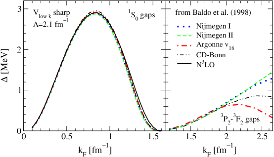
Figure 22: The ¹S₀ (left panel) and ³P${}_{2}-^{3}$F₂ (right panel) superfluid pairing gaps $\Delta$ at the Fermi surface as a function of Fermi momentum $k_{\text{F}}$ in neutron matter. The gaps are obtained from charge-dependent NN interactions at the BCS level. For details see Refs. Kai ; Baldo .

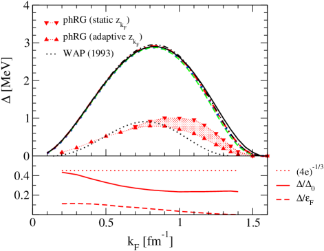
Figure 23: Top panel: Comparison of the ¹S₀ BCS gap to the results including polarization effects through the particle-hole RG (phRG), for details see Ref. RGnm , and to the results of Wambach et al. WAP2 . Lower panel: Comparison of the full superfluid gap $\Delta$ to the BCS gap $\Delta_{0}$ and to the Fermi energy $\varepsilon_{\rm F}$.

Understanding many-body effects beyond the BCS level constitutes an important open problem. For recent progress and a survey of results, see for instance Ref. Gezerlis . At low densities, induced interactions due to particle-hole screening and vertex corrections are significant even in the perturbative $k_{\text{F}}a$ limit Gorkov and lead to a reduction of the S-wave gap by a factor $(4e)^{-1/3}\approx 0.45$,

$$\frac{\Delta}{\varepsilon_{\rm F}} = \frac{8}{e^{2}}\,\exp\biggr{\{}\biggr{(}\,\begin{minipage}{125.19194pt} \includegraphics[scale={0.5},clip={}]{dilutegap.eps} \end{minipage}\biggr{)}^{-1}\biggr{\}}$$ (132)

$$= (4e)^{-1/3}\,\frac{8}{e^{2}}\,\exp\biggl{\{}\frac{\pi}{2k_{\text{F}}a}+{\mathcal{O}}(k_{\text{F}}a)\biggr{\}}\,.$$

This reduction is due to spin fluctuations, which are repulsive for spin-singlet pairing and overwhelm attractive density fluctuations.

Here, we discuss the particle-hole RG (phRG) approach to this problem using the BCS-channel-irreducible quasiparticle scattering amplitude as pairing interaction RGnm . The quasiparticle scattering amplitude is obtained, as discussed in the previous section, by solving the flow equations in the particle-hole channels, Eqs. (3) and (3), starting from $V_{{\rm low}\,k}$. This builds up many-body correlations from successive momentum shells, on top of an effective interaction with particle/hole polarization effects from all previous shells, and thereby efficiently includes induced interactions to low-lying states in the vicinity of the Fermi surface beyond a perturbative calculation.

The results for the ¹S₀ gap are shown in Fig. 23, where induced interactions lead to a factor 3–4 reduction to a maximal gap $\Delta\approx 0.8\,\text{MeV}$ RGnm . Similar values to those of Wambach et al. WAP2 are found. In addition, for the lower densities, the phRG is consistent with the dilute result $\Delta/\Delta_{0}=(4e)^{-1/3}$, and at the larger densities the dotted band indicates the uncertainty due to an approximate self-energy treatment.

Non-central spin-orbit and tensor interactions are crucial for ³P${}_{2}-^{3}$F₂ superfluidity. Without a spin-orbit interaction, neutrons would form a ³P₀ superfluid instead. The first perturbative calculation of non-central induced interactions shows that ³P₂ gaps below $10\,{\rm keV}$ are possible (while second-order contributions to the pairing interaction are not substantial $|V_{\rm ind}/V_{{\rm low}\,k}|<0.5$) tensor . This arises from a repulsive induced spin-orbit interaction due to the mixing with the stronger spin-spin interaction. As a result, neutron P-wave superfluidity (in the interior of neutron stars) may be reduced considerably below earlier estimates. This implies that low-mass neutron stars cool slowly slow . Smaller values for the ³P₂ gap compared to Fig. 22 are also required for consistency with observations in a minimal cooling scenario CasA .

4 Outlook

In these lecture notes we discussed RG approaches to Fermi liquids, based on the ideas of Shankar Shankar and Polchinski Polchinski , and formulated the flow equation in the framework of a functional RG Wetterich93 . The appeal of RG methods is that they allow a systematic study of non-perturbative correlations at different length scales. These lecture notes show that the RG approach developed for neutron matter in Ref. RGnm is equivalent to a functional RG. We reviewed results for the quasiparticle interaction and the superfluid pairing gaps in neutron matter, starting from low-momentum interactions and focusing on the effects of induced interactions due to long-range particle-hole fluctuations.

There are many important problems for RG methods applied to many-nucleon systems. These include the role of non-central interactions and of many-body forces. For example, we recently showed that novel non-central interactions are generated by polarization of the nuclear medium tensor . A non-perturbative RG treatment of these effects, which have important consequences for neutron stars, is of great interest. In recent years an alternative RG scheme, the similarity RG (SRG) SRG ; SRGnuc has emerged as a powerful tool for exploring the scale dependence of nuclear interactions and the role of many-body forces in nuclear systems. Moreover, the SRG can be applied directly to solve the many-body problem IMSRG . The SRG approach is formulated as a continuous matrix transformation acting on the Hamiltonian. An important open question is to understand the relation of the SRG to functional and field theory methods.

References

- (1) R. Shankar, Rev. Mod. Phys. 66, 129 (1994).
- (2) J. Polchinski, in Proceedings of the 1992 Theoretical Advanced Studies Institute in Elementary Particle Physics, Eds. J. Harvey and J. Polchinski (World Scientific, Singapore, 1993), hep-th/9210046.
- (3) H. Gies, lectures in this volume, hep-ph/0611146.
- (4) W. Metzner, M. Salmhofer, C. Honerkamp, V. Meden and K. Schönhammer, arXiv:1105.5289.
- (5) L. D. Landau, Sov. Phys. JETP 3, 920 (1957).
- (6) L. D. Landau, Sov. Phys. JETP 5, 101 (1957).
- (7) L. D. Landau, Sov. Phys. JETP 8, 70 (1959).
- (8) A. Larkin and A. B. Migdal, Sov. Phys. JETP 17, 1146 (1963).
- (9) A. J. Leggett, Phys. Rev. A 140, 1869 (1965); ibid. 147, 119 (1966).
- (10) G. Baym and C. J. Pethick, Landau Fermi Liquid Theory: Concepts and Applications (Wiley, New York, 1991).
- (11) A. B. Migdal, Theory of Finite Fermi Systems and Applications to Atomic Nuclei (Interscience, New York, 1967).
- (12) S.-O. Bäckman, G. E. Brown and J. Niskanen, Phys. Rept. 124, 1 (1985).
- (13) A. Schwenk and B. Friman, Phys. Rev. Lett. 92, 082501 (2004).
- (14) I. Y. Pomeranchuk, Sov. Phys. JETP 8, 361 (1959).
- (15) D. Pines and P. Nozières, The Theory of Quantum Liquids (Volume 1, Advanced Book Classics, Westview Press, 1999).
- (16) D. Vollhardt and P. Wölfle, The Superfluid Phases of Helium 3 (Taylor and Francis Ltd., London, 1990).
- (17) S. K. Bogner, T. T. S. Kuo and A. Schwenk, Phys. Rept. 386, 1 (2003); S. K. Bogner, R. J. Furnstahl and A. Schwenk, Prog. Part. Nucl. Phys. 65, 94 (2010).
- (18) A. Schwenk, B. Friman and G. E. Brown, Nucl. Phys. A 713, 191 (2003).
- (19) A. Schwenk, G. E. Brown and B. Friman, Nucl. Phys. A 703, 745 (2002).
- (20) N. Kaiser, Nucl. Phys. A 768, 99 (2006); J. W. Holt, N. Kaiser and W. Weise, Nucl. Phys. A 870-871, 1 (2011).
- (21) E. Epelbaum, H.-W. Hammer and U.-G. Meißner, Rev. Mod. Phys. 81, 1773 (2009).
- (22) S. K. Bogner, A. Schwenk, R. J. Furnstahl and A. Nogga, Nucl. Phys. A 763, 59 (2005); K. Hebeler and A. Schwenk, Phys. Rev. C 82, 014314 (2010); K. Hebeler, S. K. Bogner, R. J. Furnstahl, A. Nogga and A. Schwenk, Phys. Rev. C 83, 031301(R) (2011).
- (23) T. Otsuka, T. Suzuki, J. D. Holt, A. Schwenk and Y. Akaishi, Phys. Rev. Lett. 105, 032501 (2010); J. D. Holt, T. Otsuka, A. Schwenk and T. Suzuki, arXiv:1009.5984.
- (24) C. J. Pethick, in Lectures in Theoretical Physics, Vol. XI-B, Boulder, Colorado, 1968, Ed. K. T. Mahantappa and W. E. Brittin (Gordon and Breach, New York, 1969), p. 187.
- (25) A. L. Fetter and J. D. Walecka, Quantum Theory of Many-Particle Systems (Dover, New York, 2003).
- (26) A. A. Abrikosov, L. P. Gor’kov and I. E. Dzyaloshinski, Methods of Quantum Field Theory in Statistical Physics (Dover, New York, 1963).
- (27) J. W. Negele and H. Orland, Quantum Many-Particle Systems (Advanced Book Classics, Westview Press, 1998).
- (28) A. Altland and B. Simons, Condensed Matter Field Theory (Cambridge University Press, 2007).
- (29) A. A. Abrikosov and I. M. Khalatnikov, Rept. Prog. Phys. 22, 329 (1959).
- (30) S.-O. Bäckman, O. Sjöberg and A. D. Jackson, Nucl. Phys. A 321, 10 (1979).
- (31) B. L. Friman and A. K. Dhar, Phys. Lett. B 85, 1 (1979).
- (32) J. M. Cornwall, R. Jackiw and E. Tomboulis, Phys. Rev. D 10, 2428 (1974).
- (33) J. M. Luttinger and J. C. Ward, Phys. Rev. 118, 1417 (1960).
- (34) G. Baym, Phys. Rev. 127, 1391 (1962).
- (35) C. Wetterich, Phys. Rev. B 75, 085102 (2007).
- (36) P. Nozières, Theory of Interacting Fermi Systems (Westview Press, Boulder, 1997).
- (37) S. Babu and G. E. Brown, Ann. Phys. 78 (1973) 1.
- (38) C. Wetterich, Phys. Lett. B 301, 90 (1993).
- (39) J. Berges, N. Tetradis and C. Wetterich, Phys. Rept. 363, 223 (2002).
- (40) N. Dupuis, Eur. Phys. J. B 48, 319 (2005).
- (41) K. Hebeler, PhD Thesis, Technische Universität Darmstadt (2007).
- (42) T. M. Morris, Nucl. Phys. B 458, 477 (1996).
- (43) U. Ellwanger, Z. Physik C 62, 503 (1994).
- (44) S. K. Bogner, R. J. Furnstahl, S. Ramanan and A. Schwenk, Nucl. Phys. A 773, 203 (2006); S. Ramanan, S. K. Bogner and R. J. Furnstahl, Nucl. Phys. A 797, 81 (2007).
- (45) T. L. Ainsworth, J. Wambach and D. Pines, Phys. Lett. B 222, 173 (1989).
- (46) J. Wambach, T. L. Ainsworth and D. Pines, Nucl. Phys. A 555, 128 (1993).
- (47) S.-O. Bäckman, C.-G. Källman and O. Sjöberg, Phys. Lett. B 43, 263 (1973).
- (48) A. D. Jackson, E. Krotschek, D. E. Meltzer and R. A. Smith, Nucl. Phys. A 386, 125 (1982).
- (49) L. G. Cao, U. Lombardo and P. Schuck, Phys. Rev. C 74, 064301 (2006).
- (50) D. G. Yakovlev and C. J. Pethick, Annu. Rev. Astron. Astrophys. 42, 169 (2004); D. Blaschke, H. Grigorian and D. N. Voskresensky, Astron. Astrophys. 424, 979 (2004); D. Page, J. M. Lattimer, M. Prakash and A. W. Steiner, Astrophys. J. Suppl. 155, 623 (2004).
- (51) E. M. Cackett, R. Wijnands, M. Linares, J. M. Miller, J. Homan and W. Lewin, Mon. Not. Roy. Astron. Soc. 372, 479 (2006); E. M. Cackett, R. Wijnands, J.M. Miller, E. F. Brown and N. Degenaar, Astrophys. J. 687, L87 (2008); E. F. Brown and A. Cumming, Astrophys. J. 698, 1020 (2009).
- (52) T. Lesinski, T. Duguet, K. Bennaceur and J. Meyer, Eur. Phys. J. A 40, 121 (2009); K. Hebeler, T. Duguet, T. Lesinski and A. Schwenk, Phys. Rev. C 80, 044321 (2009); T. Lesinski, K. Hebeler, T. Duguet and A. Schwenk, J. Phys. G 39, 015108 (2012).
- (53) K. Hebeler, A. Schwenk and B. Friman, Phys. Lett. B 648, 176 (2007).
- (54) M. Baldo, O. Elgaroy, L. Engvik, M. Hjorth-Jensen and H.-J. Schulze, Phys. Rev. C 58, 1921 (1998).
- (55) A. Gezerlis and J. Carlson, Phys. Rev. C 81, 025803 (2010).
- (56) L. P. Gorkov and T. K. Melik-Barkhudarov, Sov. Phys. JETP 13, 1018 (1961); H. Heiselberg, C. J. Pethick, H. Smith and L. Viverit, Phys. Rev. Lett. 85, 2418 (2000).
- (57) F. Barranco, R. A. Broglia, G. Colo, G. Gori, E. Vigezzi and P. F. Bortignon, Eur. Phys. J. A 21, 57 (2004); A. Pastore, F. Barranco, R. A. Broglia and E. Vigezzi, Phys. Rev. C 78, 024315 (2008).
- (58) A. Schwenk and C. J. Pethick, Phys. Rev. Lett. 95, 160401 (2005).
- (59) D. Page, M. Prakash, J. M. Lattimer and A. W. Steiner, Phys. Rev. Lett. 106, 081101 (2011); P. S. Shternin, D. G. Yakovlev, C. O. Heinke, W. C. G. Ho and D. J. Patnaude, Mon. Not. Roy. Astron. Soc. 412, L108 (2011).
- (60) S. D. Glazek and K. G. Wilson, Phys. Rev. D 48, 5863 (1993); F. Wegner, Ann. Phys. (Leipzig) 3, 77 (1994).
- (61) S. K. Bogner, R. J. Furnstahl and R. J. Perry, Phys. Rev. C 75, 061001(R) (2007).
- (62) K. Tsukiyama, S. K. Bogner and A. Schwenk, Phys. Rev. Lett. 106, 222502 (2011).