Analytical properties of horizontal visibility graphs in the Feigenbaum scenario

Abstract

Time series are proficiently converted into graphs via the horizontal visibility (HV) algorithm, which prompts interest in its capability for capturing the nature of different classes of series in a network context. We have recently shown plos that dynamical systems can be studied from a novel perspective via the use of this method. Specifically, the period-doubling and band-splitting attractor cascades that characterize unimodal maps transform into families of graphs that turn out to be independent of map nonlinearity or other particulars. Here we provide an in depth description of the HV treatment of the Feigenbaum scenario, together with analytical derivations that relate to the degree distributions, mean distances, clustering coefficients, etc., associated to the bifurcation cascades and their accumulation points. We describe how the resultant families of graphs can be framed into a renormalization group scheme in which fixed-point graphs reveal their scaling properties. These fixed points are then re-derived from an entropy optimization process defined for the graph sets, confirming a suggested connection between renormalization group and entropy optimization. Finally, we provide analytical and numerical results for the graph entropy and show that it emulates the Lyapunov exponent of the map independently of its sign.

In recent years a new general framework to make time series analysis has been coined. This framework is based on the mapping of a time series into a network representation and the subsequent graph theoretical analysis of the network, offering the possibility of describing the structure of complex signals and the associated dynamical systems from a new and complementary viewpoint, and with a full set of alternative measures. Here we focus on a specific type of mapping called the horizontal visibility algorithm, and via this approach we address the specific case of the period-doubling route to chaos. We extend our preliminary results on this topic plos , and provide a complete graph theoretical characterization of unimodal iterated maps undergoing period doubling route to chaos that, we show, evidence a universal character. Our approach allows us to visualize, classify and characterize periodic, chaotic and onset of chaos dynamics in terms of their associated networks.

I Introduction

Very recently plos , a connection between nonlinear dynamical systems and complex networks has been accounted for by means of the horizontal visibility (HV) algorithm pre ; submitted , as the latter transforms time series into graphs. The families of trajectories generated by nonlinear low-dimensional iterated maps conform a distinctive class of time series. Accordingly, they make up ideal candidates to test the capabilities of the HV algorithm for capturing meaningfully the information contained in them, and, if so, see how these manifest in the network central quantities. The possibility of observation of novel properties adds to the motivation to carry on these studies. We have chosen to inspect first the well-known one-dimensional (therefore dissipative) unimodal maps and their common period-doubling route to chaos, when periodic attractors transform into aperiodic attractors, the bifurcation cascade or Feigenbaum scenario chaos ; chaos2 . This route to chaos appears an infinite number of times amongst the family of attractors generated by unimodal maps within the windows of periodic attractors that interrupt sections of chaotic attractors. In the opposite direction, a route out of chaos accompanies each period-doubling cascade by a chaotic band-splitting cascade, and their shared bifurcation accumulation points form transitions between order and chaos that possess universal properties chaos ; chaos2 ; steve . Low-dimensional dynamics benefits from added interest as systems with many degrees of freedom relevant to various problems in physics and elsewhere are known to undergo a drastic simplification and display this type of dynamics Strogatz .

There is a growing number of methods designed to transform series into networks, involving concepts such as recurrence in phase space zhang1 ; review_grafos or Markov processes amaral to cite a few, and our approach forms part of this enterprise pnas . Once a time series is converted into a network the interest lies in the observation of the characteristic properties of dynamical systems in a different environment. And to achieve this it is necessary to use the characteristic tools of network analysis stro1 ; redes ; redes2 ; redes3 ; bollobas . The family of visibility algorithms has been successful in obtaining information relevant to the description of fractal behavior epl or to the distinction between random and chaotic series submitted . Here we detail the Feigenbaum scenario as seen through the HV formalism by providing a complete description of its associated set of graphs. These graphs represent the time evolution of all trajectories that take place within the attractors of unimodal maps. The outline of the presentation is the following: We start in Section II by recalling the construction of an HV graph from a time series and deduce general expressions for the mean degree and distance when the series is periodic. We advance a visual illustration of the graphs and their location in the Feigenbaum diagram. In Section III we focus on the period-doubling cascade and derive a simple closed-form expression for the degree distribution of periodic attractor graphs and their accumulation point. We obtain from the latter the mean degree, the variance and the clustering coefficient. In Section IV we center on the reverse bifurcation cascade of chaotic-band attractors and derive the expression for the degree distribution and the mean degree. As the number of bands increases there is a growing similarity with the same quantities for the period-doubling cascade, since, as shown, the contribution from chaotic motion is confined only to the shrinking top band. The properties of graphs stemming from both chaotic-band attractors and windows of periodicity are derived with help of the self-affine properties of the bifurcation cascades. In Section V we describe a renormalization group (RG) transformation, equivalent to the original functional composition RG transformation, but specially designed for the Feigenbaum graphs, that leads to a set of fixed point graphs that further explain, and give unity to, the two previous sections. In Section VI we turn attention to the entropy associated to the degree distributions and find that under optimization we recover the RG fixed points. Finally we compare the behavior of this entropy as we move along the bifurcation cascades and notice that this quantity follows closely the variation of the map’s Lyapunov exponent, pointing out to a property reminiscent of the Pesin equality but suitable for both periodic and chaotic graphs. In Section VII we summarize our results. A brief preliminary account of the contents of this paper is given in plos .

II Feigenbaum graphs

Figure 1: Feigenbaum graphs from the Logistic map $x_{t+1}=f(x_{t})=\mu x_{t}(1-x_{t})$. The main figure portrays the family of attractors of the Logistic map and indicates a transition from periodic to chaotic behavior at $\mu_{\infty}=3.569946...$ through period-doubling bifurcations. For $\mu\geq\mu_{\infty}$ the figure shows merging of chaotic-band attractors where aperiodic behavior appears interrupted by windows that, when entered from their left-hand side, display periodic motion of period $T=m\cdot 2^{0}$ with $m>1$ (for $\mu<\mu_{\infty}$, $m=1$) that subsequently develops into $m$ period-doubling cascades with new accumulation points $\mu_{\infty}(m)$. Each accumulation point $\mu_{\infty}(m)$ is in turn the limit of a chaotic-band reverse bifurcation cascade with $m$ initial chaotic bands, reminiscent of the self-affine structure of the entire diagram. All unimodal maps exhibit a period-doubling route to chaos with universal asymptotic scaling ratios between successive bifurcations that depend only on the order of the nonlinearity of the map Feigenbaum , the Logistic map belongs to the quadratic case. Adjoining the main figure, we show time series and their associated Feigenbaum graphs according to the HV mapping criterion for several values of $\mu$ where the map evidences both regular and chaotic behavior (see the text). Inset: Numerical values of the mean normalized distance $\bar{d}$ as a function of mean degree $\bar{k}$ of the Feigenbaum graphs for $3<\mu<4$ (associated to time series of $1500$ data after a transient and a step $\delta\mu=0.05$), in good agreement with the theoretical linear relation (see the text).

The HV graph pre associated with a given time series $\{x_{i}\}_{i=1,...,N}$ of $N$ real data is constructed as follows: First, a node $i$ is assigned to each datum $x_{i}$, and then two nodes $i$ and $j$ are connected if the corresponding data fulfill the criterion $x_{i},x_{j}>x_{n}$ for all $n$ such that $i<n<j$. Let us now focus on the Logistic map chaos defined by the quadratic difference equation $x_{t+1}=f(x_{t})=\mu x_{t}(1-x_{t})$ where $x_{t}\in[0,1]$ and the control parameter $\mu\in{\rm[0,4]}$. According to the HV algorithm, a time series generated by the Logistic map for a specific value of its control parameter $\mu$ (after an initial transient of approach to the attractor) is converted into a Feigenbaum graph (see figure 1). Notice that this is a well-defined subclass of HV graphs where consecutive nodes of degree $k=2$, that is, consecutive data with the same value, do not appear, what is actually the case for series extracted from maps (besides the trivial case of a constant series). Also, as proven in simone , an HV graph is, by construction, a planar graph, that is, it has a diagram representation in which any pair of links intersect only at their endpoints. Moreover, an HV graph is also outerplanar: each node contacts the infinite face, where a face is a bounded region of a planar graph and the infinite face is its outer region. In what follows we take advantage of these facts and outline some generic properties of Feigenbaum graphs.

Mean degree $\bar{k}$.

Figure 2: Graphical illustration of the constructive proof of the expression for the mean degree $\bar{k}(T)$ through consideration of a motif extracted from a periodic series of period $T=5$. Observe that the second data is the one with the lowest value. By deleting it, the graph loses $2$ links. This process is iterated three more times. A total amount of $2\cdot(5-1)=8$ links has been deleted, independently of the inner structure of the $T=5$ motif.

Consider a periodic orbit of period $T$. Without lack of generality, we represent the orbit as the infinite time series $\{...,x_{0},x_{1},...,x_{T},x_{1},x_{2},...\}$, where $x_{0}=x_{T}$ corresponds to the largest value of the series. By construction, the associated Feigenbaum graph consists of a concatenation of identical motifs of $T+1$ nodes associated to the subseries $\{x_{0},x_{1},...,x_{T}\}$. Suppose that the motif is a graph with $V$ links, and let $x_{i}$ be the smallest datum of the subseries which, by construction, will have degree $k=2$ (and since no data repetitions are allowed in the motif, $x_{i}$ will always be well defined). Now remove this node and its two links from the motif. The resulting motif will have $V-2$ links and $T$ nodes. Iterate this operation $T-1$ times (see figure 2 for a graphical illustration of this process in a particular case with $T=5$). The resulting graph will have only two nodes, associated with $x_{0}$ and $x_{T}$, connected by a single link, and the total number of deleted links will be $2(T-1)$. The mean degree $\bar{k}$ of the graph corresponds to the mean degree of the motif made of $T$ nodes (the nodes associated with $x_{0}$ and $x_{T}$ only introduce half of their degree in the motif, what is equivalent to an effective reduction of one node). Hence,

$$\bar{k}(T)\equiv 2\frac{\#\ edges}{\#\ nodes}=\frac{2(2(T-1)+1)}{T}\Rightarrow\bar{k}(T)=4\bigg{(}1-\frac{1}{2T}\bigg{)}.$$ (1)

The above result holds for every periodic or aperiodic ($T\rightarrow\infty$) series, independent of the deterministic process that generates them, as the only constraint in its derivation is that data within a period are not repeated. It therefore includes all graphs generated by unimodal maps irrespective of their degree of nonlinearity. Observe that the maximum mean degree (achieved for aperiodic series) is $\bar{k}(\infty)=4$, in agreement with previous theory (see simone ).

Normalized mean distance $\bar{d}$. On the other hand, the normalized mean distance $\bar{d}$ of the graph is defined as $\bar{d}=\bar{D}/N$, where $\bar{D}$ is the mean distance (the average over all pairs of nodes of the smallest path that connects each pair) and $N$ the number of nodes. For graphs associated with periodic orbits $\bar{d}$ depends on $T$ (as this is the maximal amount of nodes that can be jumped through a link), and straightforwardly gives $\bar{d}(T)=\frac{1}{3T}$ for $N\rightarrow\infty$. Therefore, for HV graphs $\bar{d}$ and $\bar{k}$ are linearly related by

$$\bar{d}(\bar{k})=\frac{1}{6}(4-\bar{k}).$$ (2)

This latter analytical relation is checked numerically in the inset of figure 1. The limiting solution $\bar{k}\rightarrow 4$, $\bar{d}\rightarrow 0$ holds for all aperiodic, chaotic or random series. In addition to the numerical results shown in the inset of figure 1 for the specific case of the Logistic map, we have also examined the accuracy of the latter relation for several unimodal maps, giving perfect agreement in every case (data not shown).

III Period-doubling route to chaos: Results

Figure 3: Periodic Feigenbaum graphs for $\mu<\mu_{\infty}$. The sequence of graphs associated to periodic attractors with increasing period $T=2^{n}$ undergoing a period-doubling cascade. The pattern that occurs for increasing values of the period is related to the universal ordering with which an orbit visits the points of the attractor. Observe that the hierarchical self-similarity of these graphs requires that the graph for $n-1$ is a subgraph of that for $n$.

III.1 Order of visits of stable branches and chaotic bands

A deep-seated feature of the period-doubling cascade is that the order in which the positions of a periodic attractor are visited is universal schroeder . That is, the visiting order of the positions $\{x_{i}\}$ (where the subindex $i$ denotes the iteration time) of a periodic attractor along the period-doubling route to chaos is the same for all unimodal maps schroeder . This ordering turns out to be a decisive property in the derivation of the structure of the Feigenbaum graphs (see figure 3 where we plot the graphs for a family of attractors of increasing period $T=2^{n}$, that is, for increasing values of $\mu<\mu_{\infty}$). Here we describe the rule that such ordering follows for orbits of period $T=2^{n}$, and how this in turn induces the structure of the associated Feigenbaum graphs. This is illustrated graphically in figure 4.

Figure 4: Graphical illustration that explains how the order of visits to the stable branches of the map induces the structure of the Feigenbaum graphs all along the period-doubling bifurcation cascade ($\mu<\mu_{\infty}$).

Consider the first period-doubling bifurcation that produces attractors with period $T=2^{1}$ and for which repeated jumps are observed between two positions in time, $x_{1}$, $x_{2}$, $x_{1}$, …, with $x_{1}>x_{2}$ (figure 4.a). Without lack of generality label $x_{1}$ as the largest data. This series is transformed into a Feigenbaum graph made up of a concatenation of a root motif of $3$ nodes, where by construction the inner node is associated with datum $x_{2}$. As the family of attractors reaches the next period-doubling bifurcation, each point $x_{i}$ of the period-2 attractor splits into two new stable ‘offspring’ positions: $x_{i}$ and $x_{i+T}$, and the visiting order is such that $x_{1}>x_{3}>x_{4}>x_{2}$ (figure 4.b). This ordering is reminiscent of the $T=2^{1}$ orbit that was present before the bifurcation (namely, the orbit returns to a neighborhood of the point after a journey along the attractor). In particular, this means that the second largest value $x_{3}$ (the offspring of $x_{1}$) is visited only after a $T=2^{1}$ journey, that is, in the middle of the $T=2^{2}$ periodic orbit. Observe also that the bottom pair of offspring positions appears inverted (grey box in the figure). The corresponding Feigenbaum graph is a concatenation of the $T=2^{1}$ motif (blue and red portions in the figure) linked by the largest node $x_{1}$, which repeats after $T=2^{2}$ iteration times. Blue and red portions in the graph are equivalent since the orbit follows the same pattern of visits across the stable branches (each portion according to a given offspring). The same procedure can be iterated for increasing period-doubling bifurcations (see figure 4.c), leading to Feigenbaum graphs which are progressively self-similar and become so in the limit $n\rightarrow\infty$. Summing up, the period-doubling bifurcation of an orbit of period $T=2^{n}$ generates two identical copies of the $T=2^{n}$ root motif of the graph that are now concatenated by the node associated to datum $x_{1+2^{n}}$ and linked by the bounding nodes $x_{1}$, and this in turn is the root motif of the $T=2^{n+1}$ Feigenbaum graph. In the following section we will take advantage of this structure to analytically derive several topological properties of the Feigenbaum graphs along the period-doubling cascade.

III.2 Topological properties of Feigenbaum graphs along the period-doubling cascade

III.2.1 Degree distribution $P(n,k)$

Figure 5: Dots: Semi-log plot of the degree distribution of a Feigenbaum graph associated with a time series of $10^{6}$ data extracted from a Logistic map at the onset of chaos $\mu_{\infty}=3.5699456...$. The straight line corresponds to equation III.2.1, in agreement with the numerical calculation (the deviation for large values of the degree are due to finite size effects).

The above-described order of visits generates a hierarchy of self-similar Feigenbaum graphs along the period-doubling bifurcation cascade. The degree distribution of a graph is defined as a discrete probability distribution that expresses the probability of finding a node with degree $k$ redes ; redes2 ; redes3 . By construction, the degree distribution of a Feigenbaum graph for a series of period $T=2^{n}$, $n=0,1,2,...,$ is

$$P(n,k)=\left({\frac{1}{2}}\right)^{k/2},\quad k=2,4,6,...,2n,$$

$$P(n,k)=\left({\frac{1}{2}}\right)^{n},\quad k=2(n+1),$$

$$P(n,k)=0,\quad k=3,5,7,...,\quad\text{or}\quad k>2(n+1).$$ (3)

At the accumulation point $\mu_{\infty}=3.5699456...$ the period diverges ($n\rightarrow\infty$), and the degree distribution of the Feigenbaum graph at the onset of chaos becomes a (non truncated) exponential for even values of the degree,

$$P(\infty,k)=\left(\frac{1}{2}\right)^{k/2},\quad k=2,4,6,...,$$

$$P(\infty,k)=0,\quad k=3,5,7,...$$ (4)

In figure 5 we show the accuracy with which this analytical result is reproduced by a finite series of $10^{6}$ data. Numerical and theoretical distributions are in good agreement.

III.2.2 Mean degree $\bar{k}(n)$ and normalized distance $\bar{d}(n)$

The mean degree $\bar{k}(n)$ is the first moment of the degree distribution

$$\bar{k}(n)=\sum_{k=2}^{2(n+1)}{kP(n,k)}=4\bigg{(}1-\frac{1}{2^{n+1}}\bigg{)},$$ (5)

which at the accumulation point yields $\bar{k}(\infty)=4$, indeed the maximal degree for an HV graph.

Furthermore, by induction it can be shown that the mean distance $D(n,N)$ within a Feigenbaum graph of $N$ nodes after $n$ period-doubling bifurcations is given approximately by

$$\bar{D}(n,N)\approx\frac{1}{2^{n}}\left\{\frac{N+1}{3}+\frac{1}{9}\left[(6n-1)2^{n}+(-1)^{n}\right]\right\}.$$ (6)

Observe that for a fixed period $T=2^{n}$ the mean distance increases linearly with the size $N$ of the graph. Normalization of this measure in the limit of infinite size leads to a well-defined mean distance per node $\bar{d}(n)$ with the simple form

$$\bar{d}(n)=\frac{1}{3}\frac{1}{2^{n}},$$ (7)

such that the linear relation depicted in equation 2 is recovered.

III.2.3 Clustering coefficient $c(n,k)$

The local clustering coefficient is a topological measure that quantify how close a given node’s neighbors are to being a clique redes ; redes2 ; redes3 . The local clustering coefficient of a Feigenbaum graph that corresponds to an attractor of period $T=2^{n}$ is given by

$$c(n,k)=\frac{k-1}{{\binom{k}{2}}}=\frac{2}{k},\quad k=2,4,6,...,2n,$$

$$c(n,k)=\frac{k-2}{{\binom{k}{2}}}=\frac{2(k-2)}{k(k-1)},\quad k=2(n+1),$$ (8)

a result indicative of a so-called hierarchical structure hierar . Since the degree distribution $P(n,k)$ is known in closed form throughout the period-doubling cascade, use of the approximation $c(n,2(n+1))\approx 1/(n+1)$ leads to

$$P(n,k)=\left({\frac{1}{2}}\right)^{k/2}=P(n,2/c(n,k)),\quad k=2,4,6,...,2n,2(n+1),$$

$$P(n,c)=\left({\frac{1}{2}}\right)^{1/c}.$$ (9)

Consequently, the mean clustering coefficient $\bar{c}(n)$ is given by

$$\bar{c}(n)=\sum_{k=2}^{2(n+1)}{c(n,k)P(n,k)}=\sum_{k=2}^{2n}{\frac{2}{k}\left({\frac{1}{2}}\right)^{k/2}}+\frac{2n}{(n+1)(2n+1)}\left({\frac{1}{2}}\right)^{n}$$ (10)

$$= \sum_{m=1}^{n}{\frac{1}{m2^{m}}}+\frac{n}{2^{n-1}(n+1)(2n+1)}.$$

This last summation does not possess a solution in closed form except in the limit $n\rightarrow\infty$ which yields $\bar{c}(\infty)=\log 2=0.693..$. Nevertheless, the series converges to $\log 2$ extremely fast: $c(0)=0,c(1)=0.666...,c(2)=0.691666...,c(3)=0.693452...$, which suggests that $\bar{c}(n)$ rapidly loses its dependence on the bifurcation order $n$ and remains basically constant for all $n$.

III.2.4 Higher moments of the degree distribution: variance $\sigma^{2}(n)$

The moments of the degree distribution $P(n,k)$ can be easily calculated by making use of the generating function

$$M(t)=\langle e^{tk}\rangle=1+\left(4-\frac{2}{2^{n}}\right)t+$$

$$\left(12-\frac{10+4n}{{2}^{n}}\right){t}^{2}+\left(\frac{104}{3}-\frac{(100/3)+20n+4n^{2}}{2^{n}}\right){t}^{3}+O\left({t}^{4}\right).$$

In particular, the variance is given by

$$\sigma^{2}(n)=8-\frac{4+8n}{2^{n}}-{4}^{1-n},$$

which at the accumulation point becomes $\sigma^{2}(\infty)=8$.

IV Reverse bifurcation cascade of chaotic bands: results

Figure 6: Aperiodic Feigenbaum graphs for $\mu>\mu_{\infty}$. A sequence of graphs associated with chaotic series after $n$ chaotic-band reverse bifurcations, starting at $\mu=4$ for $n=0$, when the attractor extends along a single band and the degree distribution does not present any regularity (red links). For $n>0$ the phase space is partitioned in $2^{n}$ disconnected chaotic bands and the $n$-th self-affine image of $\mu=4$ is the $n$-th Misiurewicz point $\mu_{2^{n-1}-2^{n}}$. In all cases, the orbit visits each chaotic band in the same order as in the periodic region $\mu<\mu_{\infty}$. This order of visits induces an ordered structure in the graphs (black links) analogous to that found for the period-doubling cascade.

The Logistic map at $\mu=4$ is said to be fully chaotic as the Lyapunov exponent attains its maximum value of $\log 2$ there, and also the single-band attractor spans the unit interval. As $\mu$ is decreased smoothly from $\mu=4$ towards $\mu_{\infty}$, this first chaotic band ($n=0$) suffers a contraction and a series of successive band splittings (see figure 1) that are in several respects analogous to the period-doubling bifurcations at $\mu<\mu_{\infty}$. Since the band splittings occur from right to left, they are called reverse bifurcations chaos ; chaos2 ; steve ; schroeder . After the first reverse bifurcation ($n=1$), the first chaotic band splits into two disconnected chaotic bands, such that the iteration of an initial condition in this zone generates an orbit that alternates between these two bands. While the exact location of each position gives evidence of sensitive dependence on initial conditions the band alternation is fixed. Significantly, while in the chaotic zone orbits are aperiodic, for reasons of continuity they visit each of the $2^{n}$ chaotic bands in the same order as positions are visited in the attractors of period $T=2^{n}$ schroeder . In figure 6 we have plotted the Feigenbaum graphs generated through chaotic time series at different values of $\mu$ that correspond to an increasing number of reverse bifurcations.

Figure 7: Self-affinity in the chaotic region: the two disconnected chaotic bands at $\mu_{2-4}<\mu<\mu_{1-2}$ are rescaled copies of the first chaotic band $\mu_{1-2}<\mu<4$. An orbit at $\mu_{2-4}<\mu<\mu_{1-2}$ makes an alternating journey between both bands.

The first of the reverse bifurcation points, called Misiurewicz points, is located at $\mu_{1-2}=3.6785...$. As in the period-doubling region $\mu<\mu_{\infty}$, a cascade of chaotic band reverse bifurcations takes place in the complementary region $\mu>\mu_{\infty}$, such that after $n$ bifurcations the attractor consists of $2^{n}$ non-overlapping chaotic bands. The location of the Misiurewicz points converges to $\mu_{\infty}$ in the limit $n\rightarrow\infty$, and their relative locations also obey the same asymptotic ratio $\delta=4.669...$ (Feigenbaum constant for quadratic maps) as $n$ increases as that occurring for the period-doubling bifurcations at $\mu<\mu_{\infty}$ chaos ; grosman .
Furthermore, the chaotic bands that are formed after each reverse bifurcation are self-affine copies of the previous ones mandelbrot . This is illustrated in figure 7, where it can be observed that the two chaotic bands (blue and orange boxes) appearing after the first reverse bifurcation (at $\mu_{1-2}$) are rescaled copies of the first chaotic band (red box). Accordingly, each value of $\mu$ within the first chaotic band has $n$ self-affine images after $n$ reverse bifurcations. For instance, the first Misiurewicz point $\mu_{1-2}=3.6785...$ is a self-affine image of $\mu=4$ after the first reverse bifurcation, the second Misiurewicz point $\mu_{2-4}=3.5925...$ is also a self-affine image of $\mu=4$ after the second reverse bifurcation, and so on. Consider now a chaotic time series extracted at $\mu\in[\mu_{2-4}-\mu_{1-2}]$ in which the iterate position values alternate between both chaotic bands. Now separate this series into two time-ordered subseries, each of which contain only data belonging to either the top or the bottom chaotic bands. These subseries are indeed rescaled copies of a series extracted from the first chaotic band at the corresponding preimage value of $\mu$. Notice that the HV algorithm is invariant under affine transformations in the series. Accordingly, the Feigenbaum graphs of these subseries are the same as the graph obtained for the self-affine value of $\mu$ belonging to the first chaotic band.

IV.1 Self-affine properties of chaotic bands: mean degree and degree distribution

As mentioned, the interband motion that an orbit experiences within an attractor composed of $2^{n}$ chaotic bands follows the same order of visits as that we described for a periodic orbit of period $2^{n}$. And as in the case of the periodic region, this property possibilitates the derivation of the main characteristics of the Feigenbaum graphs in the chaotic region. Consider the Feigenbaum graph of a chaotic series generated by the Logistic map after $n$ reverse bifurcations. By construction, the structure of this graph is in many respects a mirror image of the Feigenbaum graph in the periodic region after $n$ period-doubling bifurcations. The only differences originate from the data located within the top chaotic band. This feature is due to the fact that chaotic bands do not overlap and that the HV algorithm filters out the precise locations of data in favor of unspecified relative positions. Denote by $P_{\mu}(n,k)$ its degree distribution, where, in order to not overburden the notation, we refer to $\mu$ indistinctly of the self-affine image of $\mu$ we study. By construction, and up to $k=2n$, the degree distribution $P_{\mu}(n,k)$ is equivalent to its periodic region counterpart, i.e.

$$P_{\mu}(n,k)=\left(\frac{1}{2}\right)^{k/2},\quad k=2,4,6,...,2n.$$ (11)

Now, the data belonging to the top chaotic band transmits a specific contribution to the associated Feigenbaum graph which in general cannot be determined analytically, and as we shall see shows up in $P_{\mu}(n,k)$ for $k>2n$. This contribution is denoted $P_{\mu}^{\text{top}}(n,k)$, where, by definition, $P_{\mu}^{\text{top}}(0,k)=P_{\mu}(0,k)$, the degree distribution of the Feigenbaum graph at the first chaotic band $n=0$, $\mu_{1-2}<\mu\leq 4$. While the precise shape of the $\mu$-dependent distribution $P_{\mu}^{\text{top}}(n,k)$ is unknown, the self-affine structure of the band-splitting cascade described previously makes it possible to relate it to the first chaotic band, i.e.

$$P_{\mu}^{\text{top}}(n,k)=P_{\mu}(0,k).$$

This important property, that, as we shall comment below, corresponds to a crossover phenomenon in the RG flows, breaks down the structure of the Feigenbaum graphs within the chaotic region into two contributions: (i) an interband contribution stemming from the order of visits amongst chaotic bands that is equivalent to that for periodic attractors (with associated black links in figure 6), and (ii) a contribution from the first chaotic band (with associated red links in figure 6). For normalization reasons, this second contribution can be coarse-grained as a cumulative distribution, leading to

$$P_{\mu}(n,k)=\left(\frac{1}{2}\right)^{k/2},\quad k=2,4,6,...,2n,$$

$$P_{\mu}(n,k\geq 2(n+1))=\left(\frac{1}{2}\right)^{n}.$$ (12)

Interestingly, as $n$ increases the contributions from the interband motion of the chaotic attractor these become more and more dominant and the contribution associated with the first chaotic band is progressively smeared out, disappearing at the accumulation point $\mu_{\infty}$ (see figure 6).

Based on the previous arguments on self-affinity, the contribution from the first chaotic band can be determined quantitatively as follows. For concreteness, let us focus on a chaotic attractor located after the first reverse bifurcation. The attractor is divided into two non-overlapping chaotic bands, and every orbit in it alternates between the ‘top’ and ‘bottom’ bands. While the precise location of the visits within each band is unknown, by construction the nodes associated to the data located in the ‘bottom’ band have degree $k=2$, and this occurs for half of the iteration times, so

$$P_{\mu}(1,2)=\frac{1}{2}.$$

Also, for parity reasons (even number of chaotic bands) one has

$$P_{\mu}(1,3)=0,$$

independently of $\mu$. For $k>3$, the contribution comes necessarily from the top band, and normalization yields

$$P_{\mu}(1,k)=\frac{1}{2}P_{\mu}^{\text{top}}(1,k-2),\quad k\geq 4.$$

Finally, self-affinity implies

$$P_{\mu}^{\text{top}}(1,k)=P_{\mu}(0,k).$$

Repeating this same procedure, we find that after $n$ reverse bifurcations the degree distribution of a Feigenbaum graph fulfills the expressions

$$P_{\mu}(n,k)=\left(\frac{1}{2}\right)^{k/2},\quad k=2,4,6,...,2n,$$ (13)

$$P_{\mu}(n,k)=0,\quad k=3,5,7,...,2n+1,$$ (14)

independently of $\mu$, and

$$P_{\mu}(n,k)=\left(\frac{1}{2}\right)^{n}P_{\mu}^{\text{top}}(n,k-2n)=\left(\frac{1}{2}\right)^{n}P_{\mu}(0,k-2n),\quad k\geq 2(n+1),$$ (15)

that depends on $\mu$. As expected, the last expression only depends on the structure of the first chaotic band, decreases for increasing values of $n$ and disappears in the limit $n\rightarrow\infty$.

The above expressions for $P_{\mu}(n,k)$ can be used to derive the mean degree $\bar{k}_{\mu}(n)$ of a Feigenbaum graph in the chaotic regime:

$$\bar{k}_{\mu}(n)=\sum_{k=2}^{2n}{k\left({\frac{1}{2}}\right)^{k/2}}+\left(\frac{1}{2}\right)^{n}\sum_{k=2(n+1)}^{\infty}{\ kP_{\mu}(0,k-2n)}=4\left(1-\frac{1}{2^{n}}\right)+\frac{\bar{k}_{\mu}(0)}{2^{n}}.$$ (16)

This last expression relates the mean degree after $n$ reverse bifurcations to that in the first chaotic band. Interestingly, the only solution with constant mean degree in the chaotic regime is $\bar{k}_{\mu}(0)=\bar{k}_{\mu}(n)=4$, in full agreement with the general theory.

IV.2 Periodic windows: self-affine copies of the Feingenbaum diagram

Figure 8: Zoom of the Feigenbaum diagram close to the period $m=3$ window. Starting with a period $3$ orbit, each one of the stable branches develops into a period-doubling bifurcation cascade with a new accumulation point $\mu_{\infty}(3)$, beyond which the attractor becomes chaotic, interwoven with periodic windows: each part of the diagram is indeed a rescaled copy of the full Feigenbaum tree. The locations of several Feigenbaum graphs (with the notation defined in the text) within the period three window are depicted.

The Feigenbaum diagram shows a rich self-affine structure: periodic windows of initial period $m$ that undergo successive period-doubling bifurcations with new accumulation points $\mu_{\infty}(m)$ appear interwoven with chaotic attractors at $\mu>\mu_{\infty}$. These period-doubling cascades taking place beyond $\mu_{\infty}$ are self-affine copies of the fundamental period-doubling route to chaos ($\mu<\mu_{\infty}$). For instance, the window that initiates with period $m=3$ ($\mu\approx 3.84$) generates three period-doubling cascades, each one being a properly rescaled copy of the fundamental one (see figure 8 for a graphical illustration). In order to take into account such phenomenology in the labeling of Feigenbaum graphs, we make use of the following notation: $G(m,n)$ is the Feigenbaum graph associated with a periodic attractor of period $T=m\cdot 2^{n}$, that is, the graph belonging to a periodic window of initial period $m$, after $n$ period-doubling bifurcations. Observe that the process of chaotic band reverse bifurcations that take place from $\mu=4$ towards $\mu_{\infty}$ is again repeated in a self-affine manner, indeed, each accumulation point $\mu_{\infty}(m)$ is the limiting value of a chaotic-band reverse bifurcation cascade. In figure 8 this aspect is also illustrated. Accordingly, we may also extend the notation of Feigenbaum graphs belonging to chaotic regions, such that $G_{\mu}(m,n)$ is associated with a chaotic attractor composed by $m\cdot 2^{n}$ bands (that is, after $n$ reverse bifurcations of $m$ initial chaotic bands).

Given a periodic window with initial period $m$ within the first chaotic band ($\mu_{1-2}<\mu\leq 4$), we note that after $n$ reverse bifurcations, the chaotic-band attractors contain a self-affine image of that window, where there is an initial periodic attractor of period $m\cdot 2^{n}$ developing into $m\cdot 2^{n}$ period-doubling cascades inside the window. In this case, equation 16 reads

$$\bar{k}_{\mu}(n,m\cdot 2^{n})=4\left(1-\frac{1}{2^{n}}\right)+\frac{\bar{k}_{\mu}(0,m)}{2^{n}},$$

that together with equation 1 yields

$$\bar{k}_{\mu}(n,m\cdot 2^{n})=4\bigg{(}1-\frac{1}{2(m2^{n})}\bigg{)},$$

as expected.

V Renormalization Group approach

Figure 9: Renormalization process and network RG flow structure. (a) Illustration of the renormalization process $\cal R$: a node with degree $k=2$ is coarse-grained with one of its neighbors (indistinctively) into a block node that inherits the links of both nodes. This process coarse-grains every node with degree $k=2$ present at each renormalization step. (b) Example of an iterated renormalization process in a sample Feigenbaum graph at a periodic window with initial period $m=9$ after $n=2$ period-doubling bifurcations (an orbit of period $T=m\cdot 2^{n}=36$). (c) RG flow diagram, where $m$ identifies the periodic window that is initiated with period $m$ and ñ designates the order of the bifurcation, ñ $=n+1$ for period-doubling bifurcations and ñ $=-(n+1)$ for reverse bifurcations. $\Delta\mu(m)=\mu_{\infty}(m)-\mu$ denotes the reduced control parameter of the map, and $\mu_{\infty}(m)$ is the location of the accumulation point of the bifurcation cascades within that window. Feigenbaum graphs associated with periodic series ($\Delta\mu(m)>0$, ñ $>0$) converge to $G(1,0)\equiv G_{0}$ under the RG, whereas those associated with aperiodic ones ($\Delta\mu(m)<0$, ñ $<0$) converge to $G_{\text{rand}}$. The accumulation point $\mu_{\infty}\equiv\mu_{\infty}(1)$ corresponds to the unstable (nontrivial) fixed point $G(1,\infty)\equiv G_{\infty}$ of the RG flow, which is nonetheless approached through the critical manifold of graphs $G(m,\infty)$ at the accumulation points $\mu_{\infty}(m)$. In summary, the nontrivial fixed point of the RG flow is only reached via the family of the accumulation points, otherwise the flow converges to trivial fixed points for periodic or chaotic regions.

V.1 RG transformation: definition, flows and fixed points

In order to recast previous findings in the context of the renormalization group, let us define an RG operation $\cal R$ on a graph as the coarse-graining of every couple of adjacent nodes where one of them has degree $k=2$ into a block node that inherits the links of the previous two nodes (see figure 9.a). This is a real-space RG transformation on the Feigenbaum graph newmannRG , dissimilar from recently suggested box-covering complex network renormalization schemes rg ; rg2 ; rg3 . As a matter of fact, this scheme turns out to be equivalent for $\mu<\mu_{\infty}$ to the construction of an HV graph from the composed map $f^{(2)}$ instead of the original $f$, in correspondence to the original Feigenbaum renormalization procedure Feigenbaum ; steve . We first note that ${\cal R}\{G(1,n)\}=G(1,n-1)$, thus, an iteration of this process yields an RG flow that converges to the (1st) trivial fixed point ${\cal R}^{(n)}\{G(1,n)\}=G(1,0)\equiv G_{0}={\cal R}\{G_{0}\}$. This is the stable fixed point of the RG flow $\forall\mu<\mu_{\infty}$. We note that there is only one relevant variable in our RG scheme, represented by the reduced control parameter $\Delta\mu=\mu_{\infty}-\mu$, hence, to identify a nontrivial fixed point we set $\Delta\mu=0$ or equivalently $n\to\infty$, where the structure of the Feigenbaum graph turns to be completely self-similar under $\cal R$. Therefore we conclude that $G(1,\infty)\equiv G_{\infty}$ is the nontrivial fixed point of the RG flow, ${\cal R}\{G_{\infty}\}=G_{\infty}$. In connection with this, let $P_{t}(k)$ be the degree distribution of a generic Feigenbaum graph $G_{t}$ in the period-doubling cascade after $t$ iterations of $\cal R$, and point out that the RG operation, ${\cal R}\{G_{t}\}=G_{t+1}$, implies a recurrence relation $(1-P_{t}(2))P_{t+1}(k)=P_{t}(k+2)$, whose fixed point coincides with the degree distribution found in equation III.2.1. This confirms that the nontrivial fixed point of the flow is indeed $G_{\infty}$.

Next, under the same RG transformation, the self-affine structure of the family of chaotic attractors yields ${\cal R}\{G_{\mu}(1,n)\}=G_{\mu}(1,n-1)$, generating a RG flow that converges to the Feigenbaum graph associated to the 1st chaotic band, ${\cal R}^{(n)}\{G_{\mu}(1,n)\}=G_{\mu}(1,0)$. Repeated application of $\cal R$ breaks temporal correlations in the series, and the RG flow leads to a 2nd trivial fixed point ${\cal R}^{(\infty)}\{G_{\mu}(1,0)\}=G_{\text{rand}}={\cal R}\{G_{\text{rand}}\}$, where $G_{\text{rand}}$ is the HV graph generated by a purely uncorrelated random process. This graph has a universal degree distribution $P(k)=(1/3)(2/3)^{k-2}$, independent of the random process underlying probability density (see pre ; submitted ).

Finally, let us consider the RG flow inside a given periodic window of initial period $m$. As the renormalization process addresses nodes with degree $k=2$, the initial applications of $\cal R$ only change the core structure of the graph associated with the specific value $m$ (see figure 9.b for an illustrative example). The RG flow will therefore converge to the 1st trivial fixed point via the initial path ${\cal R}^{(p)}\{G(m,n)\}=G(1,n)$, with $p\leq m$, whereas it converges to the 2nd trivial fixed point for $G_{\mu}(m,n)$ via ${\cal R}^{(p)}\{G_{\mu}(m,n)\}=G_{\mu}(1,n)$. In the limit of $n\rightarrow\infty$ the RG flow proceeds towards the nontrivial fixed point via the path ${\cal R}^{(p)}\{G(m,\infty)\}=G(1,\infty)$. Incidentally, extending the definition of the reduced control parameter to $\Delta\mu(m)=\mu_{\infty}(m)-\mu$, the family of accumulation points is found at $\Delta\mu(m)=0$. A complete schematic representation of the RG flows can be seen in figure 9.c.

Interestingly, and at odds with standard RG applications to (asymptotically) scale-invariant systems, we find that invariance at $\Delta\mu=0$ is associated in this instance to an exponential (rather than power-law) function of the observables, concretely, that for the degree distribution. The reason is straightforward: ${\cal R}$ is not a conformal transformation (i.e. a scale operation) as in the typical RG, but rather, a translation procedure. The associated invariant functions are therefore non homogeneous (with the property $\text{g}(ax)=b\text{g}(x)$), but exponential (with the property $\text{g}(x+a)=c\text{g}(x)$).

V.2 Crossover phenomenon

When the RG transformation for a Feigenbaum graph is applied repeatedly, it generates flows terminating at two different trivial fixed points $G(1,0)\equiv G_{0}$ and $G_{\text{rand}}$ or at a nontrivial fixed point $G(1,\infty)\equiv G_{\infty}$. $G_{0}$ is a chain graph where every node has two links, $G_{\text{rand}}$ is a graph associated with a purely random uncorrelated process, whereas $G_{\infty}$ is a self-similar graph that represents the onset of chaos. The RG properties within the periodic windows are incorporated into a general RG flow diagram (see figure 9.c and figure 10 for an alternative representation). Here we add a comment on the standard presence of crossover phenomena in the RG applications, in our case for large $n$ (or $\mu\simeq\mu_{\infty}$) for both $\mu<\mu_{\infty}$ and $\mu>\mu_{\infty}$. In both cases the graphs $G(1,n-j)$ and $G_{\mu}(1,n-j)$ with $j\ll n$ closely resemble the self-similar $G_{\infty}$ (obtained only when $\mu=\mu_{\infty}$) for a range of values of the number $j$ of repeated applications of the transformation $\cal R$ until a clear departure takes place towards $G_{0}$ or $G_{\text{rand}}$ when $j$ becomes comparable to $n$. Hence, for instance the graph ${\cal R}^{(j)}\{G_{\mu}(1,n)\}$ will only show its true chaotic nature (and therefore converge to $G_{\text{rand}}$) once $j$ and $n$ are of the same order. In other words, this happens once its degree distribution becomes dominated by the contribution of $P_{\mu}^{\text{top}}(n,k)$ (alternatively, once the graph core -related to the chaotic band structure and the order of visits to chaotic bands- is removed by the iteration of the renormalization process).

Figure 10: Illustrative cartoon incorporating the RG flow of Feigenbaum graphs along the entire Feigenbaum diagram: aperiodic (chaotic or random) series generate graphs whose RG flow converges to the trivial fixed point $G_{\text{rand}}$, whereas periodic series (both in the region $\mu<\mu_{\infty}$ and inside periodic windows) generate graphs whose RG flow converges to the trivial fixed point $G(0,1)$. The nontrivial fixed point of the RG flow $G(\infty,1)$ is only reached through the critical manifold of graphs at the accumulation points $\mu_{\infty}(m)$.

VI Network entropy

VI.1 Entropy optimization and RG fixed points

Recently robledo , it has been point out that there exists a connection between the extremal properties of entropy expressions and the renormalization group approach, when applied to systems with scaling symmetry. Namely, that the fixed points of RG flows can be obtained through a process of entropy optimization, providing the RG approach a variational flavor. In this section we investigate on this connection, and derive, via optimization of an entropic functional for the Feigenbaum graphs, all the RG flow directions and fixed points directly from the information contained in the degree distribution. We depart by applying Jayne’s principle of Maximum Entropy jaynes with two different restrictions and prove that the degree distribution $P(k)$ that maximizes its entropy $h$ is in each case related to the fixed points of the RG flow. We employ the standard optimization technique that involves Lagrange multipliers.

Let us begin by defining a graph entropy as the Shannon entropy of the graph degree distribution

$$h=-\sum_{k=2}^{\infty}{P(k)\log{P(k)}},$$ (17)

and assume that the degree distribution ${P(k)}$ has a well-defined mean $\bar{k}$ (this is true in general for HV graphs and in particular for Feigenbaum graphs according to equation 1). The, consider the Lagrangian

$$\mathcal{L}=-\sum_{k=2}^{\infty}{P(k)\log{P(k)}}-(\lambda_{0}-1)\left(\sum_{k=2}^{\infty}{P(k)}-1\right)-\lambda_{1}\left(\sum_{k=2}^{\infty}{kP(k)}-\bar{k}\right),$$

for which the extremum condition reads

$$\frac{\partial\mathcal{L}}{\partial P(k)}=-\log{P(k)}-\lambda_{0}-\lambda_{1}k=0,$$

and has the general solution

$$P(k)=e^{-\lambda_{0}-\lambda_{1}k}.$$

The Lagrange multipliers $\lambda_{0}$ and $\lambda_{1}$ can be calculated from their associated constraints. First, the normalization of the probability density,

$$\sum_{k=2}^{\infty}{e^{-\lambda_{0}-\lambda_{1}k}}=1,$$

implies the following relation between $\lambda_{0}$ and $\lambda_{1}$

$$e^{\lambda_{0}}=\sum_{k=2}^{\infty}{e^{-\lambda_{1}k}}=\frac{e^{-\lambda_{1}}}{e^{\lambda_{1}}-1},$$

and differentiation of this last expression with respect to $\lambda_{1}$ yields

$$-\sum_{k=2}^{\infty}{ke^{-\lambda_{1}k}}=\frac{e^{-\lambda_{1}}-2}{(e^{\lambda_{1}}-1)^{2}}.$$

Second, the assumption that the mean degree is a well-defined quantity (true for HV graphs) yields

$$\sum_{k=2}^{\infty}{ke^{-\lambda_{0}-\lambda_{1}k}}=\bar{k}=\frac{2-e^{-\lambda_{1}}}{1-e^{-\lambda_{1}}}.$$

Combining the above results we find

$$\lambda_{1}=\log\left(\frac{\bar{k}-1}{\bar{k}-2}\right),$$

and

$$\lambda_{0}=\log\left(\frac{(\bar{k}-2)^{2}}{\bar{k}-1}\right).$$

Hence, the degree distribution that maximizes $h$ is

$$P(k)=\frac{\bar{k}-1}{(\bar{k}-2)^{2}}\left(\frac{\bar{k}-2}{\bar{k}-1}\right)^{k},$$

which is an increasing function of $\bar{k}$. The maximal entropy is therefore found for the maximal mean degree $\bar{k}=4$, with an associated degree distribution

$$P(k)=\frac{3}{4}\left(\frac{2}{3}\right)^{k}=\frac{1}{3}\left(\frac{2}{3}\right)^{k-2}.$$

Remarkably, we conclude that the HV graph with maximal entropy is that associated with a purely uncorrelated random process, and coincides with $G_{\text{rand}}$, a trivial fixed point of the RG flow.

Observe now that, by construction, the Feigenbaum graphs along the period-doubling route to chaos ($\mu<\mu_{\infty}$) do not have odd values for the degree. Let us assume this additional constraint in the former entropy optimization procedure. The derivation proceeds along similar steps, although summations now run only over even terms. Concretely, we have

$$e^{\lambda_{0}}=\sum_{k=1}^{\infty}{e^{-\lambda_{1}2k}}=\frac{1}{e^{2\lambda_{1}}-1},$$

which after differentiation over $\lambda_{1}$ gives

$$\sum_{k=1}^{\infty}{ke^{-\lambda_{1}2k}}=\frac{e^{2\lambda_{1}}-2}{(e^{2\lambda_{1}}-1)^{2}}$$

and

$$\sum_{k=1}^{\infty}{2ke^{-\lambda_{0}-\lambda_{1}2k}}=\bar{k}=\frac{2e^{2\lambda_{1}}}{e^{2\lambda_{1}}-1}.$$

We obtain for the Lagrange multipliers

$$\lambda_{1}=\frac{1}{2}\log\left(\frac{\bar{k}}{\bar{k}-2}\right)$$

and

$$\lambda_{0}=\log\left(\frac{\bar{k}-2}{2}\right).$$

The degree distribution that maximizes the graph entropy turns now to be

$$P(k)=\frac{2}{\bar{k}-2}\left(\frac{\bar{k}-2}{\bar{k}}\right)^{k/2}.$$

As before, entropy is an increasing function of $\bar{k}$, attaining its larger value for the upper bound value $\bar{k}=4$, which reduces to $P(k)=\left(1/2\right)^{k/2}$, $k=2,4,6,...$, equation III.2.1. We conclude that the maximum entropy of the entire family of Feigenbaum graphs, if we require that odd values for the degree are not allowed, is achieved at the accumulation point, that is, the nontrivial fixed point of the RG flow.
Finally, the network entropy is trivially minimized for a degree distribution $P(2)=1$, that is, at the trivial fixed point $G_{0}$. These results indicate that the fixed point structure of a RG flow can be obtained from an entropy optimization process, confirming the aforementioned connection.

VI.2 Network entropy and Pesin theorem

VI.2.1 Periodic attractors

By making use of the expression we have for the degree distribution $P(n,k)$ in the region $\mu<\mu_{\infty}$ we obtain for the graph entropy $h(n)$, after the $n$-th period-doubling bifurcation, the following result

$$h(n)=-\sum_{k=2}^{2(n+1)}{P(n,k)\log P(n,k)}$$ (18)

$$= -\sum_{k=2}^{2n}{\frac{1}{2^{k/2}}\log\left(\frac{1}{2^{k/2}}\right)}-\frac{1}{2^{n}}\log\left(\frac{1}{2^{n}}\right)=\frac{\log 2}{2}(\bar{k}-\frac{2}{2^{n}})=\log 4\left(1-\frac{1}{2^{n}}\right).$$

We observe that the entropy increases with $n$ and, interestingly, depends linearly on the mean degree $\bar{k}$. This linear dependence between $h$ and $\bar{k}$ is related to the fact that, generally speaking, the entropy and the mean of a probability distribution are proportional for exponentially distributed functions, a property that holds exactly in the accumulation point (eq.III.2.1) and approximately in the periodic region (eq.III.2.1), where there is a finite cut off that ends the exponential law. Interestingly, HV graphs associated with chaotic series have also been found to have an asymptotically exponential degree distribution submitted . Finally, note that in the limit $n\rightarrow\infty$ (accumulation point) the entropy converges to a finite value $h(\infty)=\log 4$.

VI.2.2 Chaotic attractors

For Feigenbaum graphs $G_{\mu}(1,n)$ (in the chaotic region), in general $h$ cannot be derived exactly since the precise shape of $P(k)$ is unknown (albeit the asymptotic shape is also exponential submitted ). However, arguments of self-affinity similar to those used for describing the degree distribution of Feigenbaum graphs can be employed in order to find some regularity properties of the entropy $h_{\mu}(n)$. Concretely, the entropy after $n$ chaotic band reverse bifurcations can be expressed as a function of $n$ and of the entropy in the first chaotic band $h_{\mu}(0)$. Using the expression for the degree distribution, a little algebra yields

$$h_{\mu}(n)=\log 4+\frac{h_{\mu}^{\text{top}}(n)}{2^{n}}=\log 4+\frac{h_{\mu}(0)}{2^{n}}.$$

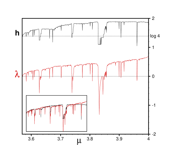
Figure 11: Horizontal visibility network entropy $h$ and Lyapunov exponent $\lambda$ for the Logistic map. We plot the numerical values of $h$ and $\lambda$ for $3.5<\mu<4$ (the numerical step is $\delta\mu=5\cdot 10^{-4}$ and in each case the processed time series have a size of $2^{12}$ data). The inset reproduces the same data but with a rescaled entropy $h-\log(4)$. The surprisingly good match between both quantities is reminiscent of the Pesin identity (see text). Unexpectedly, the Lyapunov exponent within the periodic windows ($\lambda<0$ inside the chaotic region) is also well captured by $h$.

In figure 1 we observe how the chaotic-band reverse bifurcation process takes place in the chaotic region from right to left, and therefore leads in this case to a decrease of entropy with an asymptotic value of $\log 4$ for $n\rightarrow\infty$ at the accumulation point. These results suggest that the graph entropy behaves qualitatively as the map’s Lyapunov exponent $\lambda$, with the peculiarity of having a shift of $\log 4$, as confirmed numerically in figure 11. This unexpected qualitative agreement is reasonable in the chaotic region in view of the Pesin theorem chaos2 , that relates the positive Lyapunov exponents of a map with its Kolmogorov-Sinai entropy (akin to a topological entropy) that for unimodal maps reads $h_{KS}=\lambda,\ \forall\lambda>0$, since $h$ can be understood as a proxy for $h_{KS}$. Unexpectedly, this qualitative agreement seems also valid in the periodic windows ($\lambda<0$), since the graph entropy is positive and approximately varies with the value of the associated (negative) Lyapunov exponent even though $h_{KS}=0$, hinting at a Pesin-like relation valid also out of chaos which deserves further investigation. The agreement between both quantities lead us to conclude that the Feigenbaum graphs capture not only the period-doubling route to chaos in a universal way, but also inherits the main feature of chaos, i.e. sensitivity to initial conditions.

VII Summary

In summary, we have described how the horizontal visibility algorithm transforms nonlinear dynamics into networks, in particular how the entire Feigenbaum scenario manifests in network language. The most important quality of the HV algorithm when applied to this category of time series is that it leads to definite and unique results, to well-defined families of graphs and to analytic expressions for their main property, the degree distribution. In obtaining these results two basic ingredients played a decisive role; these are the predetermined order in which positions or bands are visited in the time series and the self-affinity of periodic or chaotic-band attractors. As we have seen, the graphs generated by the algorithm store in the connectivity pattern amongst nodes, i.e. in their topological structure, the dynamical nature of the nonlinear map. A significant feature of the Feigenbaum graphs is their evident universality as the structure of all graphs and that of all families they form is independent of the specific form of the unimodal map including the degree of nonlinearity of its extremum. We have also shown that the families of networks and degree distributions obtained from periodic and chaotic attractor bifurcation cascades have scale-invariant limiting forms. And that the latter occupy the dominant positions of RG fixed points and extrema of the entropy associated with the degree distribution. The capability of the HV algorithm to expose new information is indicated by the property of the network entropy to emulate the Lyapunov exponent for both periodic and chaotic attractors. Applications of this approach to other low-dimensional nonlinear circumstances, such as the dynamical complexity associated with the quasiperiodic route to chaos and the vanishing of Lyapunov exponents are under study, and an obvious open question is how well would these precise analytical results work for experimental data.

Acknowledgments
The authors acknowledge suggestions from anonymous referees. BL and LL acknowledge financial support from the MEC and Comunidad de Madrid (Spain) through projects FIS2009-13690 and S2009ESP-1691. FJB acknowledges support from MEC through project AYA2006-14056, and AR acknowledges support from MEC (Spain) and CONACyT and DGAPA-UNAM (Mexican agencies).

References

- (1) Luque, B., Lacasa, L., Ballesteros, F. & Robledo, A., Feigenbaum graphs: a complex network description of chaos. PLoS ONE 6, 9 (2011).
- (2) Luque, B., Lacasa, L., Ballesteros, F. & Luque, J., Horizontal visibility graphs: exact results for random time series. Phys. Rev. E 80 (2009) 046103.
- (3) Lacasa, L. & Toral, R. Description of stochastic and chaotic series using visibility graphs. Phys. Rev. E 82, 036120 (2010).
- (4) Schuster, H.G. Deterministic Chaos. An Introduction (2nd revised edn, Weinheim: VCH, 1988).
- (5) Peitgen, H.O., Jurgens, H. & Saupe, D. Chaos and Fractals: New Frontiers of Science (Springer-Verlag, New York, 1992).
- (6) Strogatz S.H., Nonlinear dynamics and chaos (Perseus Books Publishing, LLC, 1994).
- (7) Marvel, S. A., Mirollo, R.E. & Strogatz, S., Identical phase oscillators with global sinusoidal coupling evolve by Möbius group action. Chaos 19, 043104 (2009).
- (8) Lacasa, L., Luque, B., Ballesteros, F., Luque, J. & Nuno, J.C., From time series to complex networks: the visibility graph. Proc. Natl. Acad. Sci. U.S.A. 105, 13 (2008) 4973.
- (9) Zhang, J. & Small, M., Complex Network from Pseudoperiodic Time Series: Topology versus Dynamics. Phys. Rev. Lett. 96, 238701 (2006).
- (10) R. V. Donner, M. Small, J. F. Donges, N. Marwan, Y. Zou, R. Xiang, J. Kurths, Recurrence-based time series analysis by means of complex network methods. Int. J. Bif. Chaos, 21(4), 1019 1046 (2011).
- (11) Campanharo, A.S. L. O., Sirer, M.I. I, Malmgren, R.D., Ramos, F.M. & Amaral, L.A.N., Duality between Time Series and Networks. PLoS ONE, 6, 8 (2011).
- (12) Strogatz, S.H., Exploring complex networks. Nature 410, 268-276 (2001).
- (13) Barabasi A,-L. & Albert R., Statistical mechanics of complex networks. Rev. Mod. Phys. 74, 47 (2002).
- (14) Newman M.E.J., The structure and function of complex networks. SIAM Rev. 45, 167 (2003).
- (15) S. Boccaletti, V. Latora, Y. Moreno, M. Chavez, and D. U. Hwang, Complex networks: Structure and dynamics. Phys. Rep. 424, 175 (2006).
- (16) B. Bollobas, Modern Graph Theory (Springer-Verlag, New York, 1998).
- (17) Lacasa, L., Luque, B., Luque, J. & Nuno, J.C., The Visibility Graph: a new method for estimating the Hurst exponent of fractional Brownian motion. EPL 86 (2009) 30001.
- (18) Gutin, G., Mansour, T. & Severini, S. A characterization of horizontal visibility graphs and combinatorics on words. arXiv:1010.1850v1.
- (19) Feigenbaum, M.J., Quantitative universality for a class of nonlinear transformations. J. Stat. Phys. 19, 25 (1978); The universal metric properties of nonlinear transformations. J. Stat. Phys. 21 (1979) 669.
- (20) Schroeder, M. Fractals, chaos, power laws: minutes from an infinite paradise (Freema and Co., New York, 1991).
- (21) Ravasz E., Somera A. L., Mongru D. A., Oltvai Z. N., & A.-L. Barabasi, Hierarchical Organization of Modularity in Metabolic Networks. Science 297, 1551 (2002).
- (22) Grosman, S., & Thomae S, Invariant distributions and stationary correlation functions of one-dimensional discrete processes. Zeitschrift fur Naturforschung 32 (1977) 1353-1363.
- (23) Crutchfield J.P., Farmer J.D. & Huberman B.A., Fluctuations and simple chaotic dynamics. Phys. Rep. 92, 2 (1982).
- (24) Newmann, M.E.J. & Watts, D.J. Renormalization group analysis of the small-world network model. Phys. Lett. A 263 (1999) pp. 341-346.
- (25) Song C., Havlin S., & Makse H.A., Self-similarity of complex networks. Nature 433 392 (2005).
- (26) Song C., Havlin S., & Makse H.A., Origins of fractality in the growth of complex networks. Nat. Phys. 2 (2006).
- (27) Radicchi F., Ramasco J.J., Barrat A., & Fortunato S., Complex Networks Renormalization: Flows and Fixed Points. Phys. Rev. Lett. 101, 148701 (2008).
- (28) Robledo, A., Renormalization group, entropy optimization, and nonextensivity at criticality. Phys. Rev. Lett. 83, 12 (1999).
- (29) E.T. Jaynes, Phys. Rev. 106, 4 (1957).