Nomads of the Galaxy

Abstract

We estimate that there may be up to $\sim 10^{5}$ compact objects in the mass range $10^{-8}-10^{-2}M_{\odot}$ per main sequence star that are unbound to a host star in the Galaxy. We refer to these objects as nomads; in the literature a subset of these are sometimes called free-floating or rogue planets. Our estimate for the number of Galactic nomads is consistent with a smooth extrapolation of the mass function of unbound objects above the Jupiter-mass scale, the stellar mass density limit, and the metallicity of the interstellar medium. We analyze the prospects for detecting nomads via Galactic microlensing. The Wide-Field Infrared Survey Telescope (WFIRST) will measure the number of nomads per main sequence star greater than the mass of Jupiter to $\sim 13\%$, and the corresponding number greater than the mass of Mars to $\sim 25\%$. All-sky surveys such as Gaia and LSST can identify nomads greater than about the mass of Jupiter. We suggest a dedicated drift scanning telescope that covers approximately 100 square degrees in the Southern hemisphere could identify nomads as small as $10^{-8}M_{\odot}$ via microlensing of bright stars with characteristic lightcurve timescales of a few seconds.

1. Introduction

The recent years have witnessed a rapid rise in the number of known planetary mass objects, $\lesssim 0.01M_{\odot}$, in the Galaxy. Searches for exoplanets from radial velocities find that $\sim 30-50\%$ of GK dwarf stars have planets greater than the mass of Neptune within periods $<50$ days (Wolfgang & Laughlin 2011). Transiting searches find that $\sim 15\%$ of main sequence dwarfs are orbited by short-period planets at less than four Earth-radii  (Borucki et al. 2010). Direct imaging and microlensing have also now started to uncover planets bound to host stars  (Gaudi 2010).

Much less is known about the population of $\lesssim 0.01M_{\odot}$ objects that are not bound to a host star. Several candidate unbound objects have been imaged in star clusters with mass possibly as small as a few times that of Jupiter, $10^{-3}M_{\odot}$ (e.g. Jayawardhana & Ivanov (2006); Caballero et al. (2007); Bihain et al. (2009)). However, the origin of these objects is uncertain; they may have formed directly in the collapse of the molecular cloud (Rees 1976), or have been ejected from their birthplace around a host star via a dynamical interaction  (Boss 2000). Free-floating objects at the Jupiter mass and below have been difficult to find via these methods.

Microlensing, however, does provide a way—and perhaps the only way—to detect objects below the deuterium-burning mass limit that are not bound to a host star. In a recent survey of the Galactic bulge, the MOA-II collaboration (Sumi et al. 2011) reported the discovery of planetary-mass objects either very distant from their host star ($\sim 100$ AU) or unbound from a host star entirely. This detection was obtained from analysis of the timescale distribution of the microlensing events, which showed a statistically-significant excess of events with timescale $\lesssim 2$ days as compared to a standard Galactic model with a stellar mass function cut-off at the low mass end of the brown dwarf regime. The mass function of this new population of objects can be described (for illustration) by a $\delta$-function with a best fit near the Jupiter mass. These results tell the surprising story that objects greater than about the mass of Jupiter are approximately twice as numerous as both main sequence stars and planets bound to host stars.

Though their existence is established, the origin of these unbound objects is far from clear. Do they form a continuation of the low end brown dwarf mass function near the deuterium burning mass limit, or did they form as a distinct population of objects ejected from their original host stars? Because of their uncertain origin and their present status, we prefer to refer to objects with mass $<0.01M_{\odot}$ that are not bound to a host star as Nomads; in the literature they have been also referred to as rogue or free-floating planets. The name “nomad” is invoked to include that allusion that there may be an accompanying “flock,” either in the form of a system of moons (Debes & Sigurdsson 2007) or in its own ecosystem. Though an interstellar object might seem an especially inhospitable habitat, if one allows for internal radioactive or tectonic heating and the development of a thick atmosphere effective at trapping infrared heat  (Stevenson 1999; Abbot & Switzer 2011), and recognizes that most life on Earth is bacterial and highly adaptive, then the idea that interstellar (and, given the prevalence of debris from major galaxy mergers, intergalactic) space is a vast ecosystem, exchanging mass through chips from rare direct collisions, is intriguing with obvious implications for the instigation of life on earth.

Understanding the bounds on the nomad population, and the prospects for detecting them with microlensing surveys, is the focus of this paper. In particular, what is the number and mass density of nomads in the Galaxy? What are the bounds on the minimum mass of a nomad, and what is the lightest detectable nomad? How well can we measure the nomad mass function, and how does this compare to the low mass brown dwarf mass function? And can we independently measure the mass function of nomads in the bulge and in the disk?

We will show that a dedicated space-based survey of the inner Galaxy, such as the proposed Wide-Field Infrared Survey Telescope (WFIRST ), will measure the number of nomads per main sequence star greater than the mass of Jupiter to $\sim 13\%$, and the corresponding number greater than the mass of Mars to $\sim 25\%$. We also show that large scale Galaxy surveys, in particular the Gaia  mission and the Large Synoptic Survey Telescope (LSST ), will be sensitive to nomads greater than about the mass of Jupiter without changing their proposed observing plan. Further, the back-to-back 15 second exposures in the planned design of LSST will allow for limits at least to be placed on nomads near the mass of Pluto, $\lesssim 10^{-8}M_{\odot}$. As an extension, we suggest that a dedicated drift scanning telescope could identify nomads as small as $10^{-8}M_{\odot}$ via microlensing of bright stars with characteristic lightcurve timescales of a few seconds.

This paper is organized as follows. In Section 2 we estimate the number of nomads in the Galaxy. In Section 3 we calculate the event rate of nomads in microlensing surveys. In Section 4 and Section 5 we outline methods for measuring the nomad population and simulating detection efficiencies. In Section 6 we present the results of these projections. In Section 7 we postulate a survey for short timescale nomads via a drift scanning telescope. In Section 8 we summarize our conclusions.

2. The Nomadic population

We begin by setting up the model for the nomad population. Objects with mass $<10^{-2}M_{\odot}$ are believed to originate from two distinct processes. Between the Jupiter mass and the deuterium-burning mass, many of these objects may form similar to stars by gravitational fragmentation. Below Jupiter masses, they likely are born in protoplanetary disks and dynamically-ejected during the evolution of the system. It is unknown from a theoretical perspective whether there is a smooth continuation of the mass function at the dividing mass that separates these populations.

In light of these uncertainties, we choose a simple broken power-law model for the nomad mass function, $dN/dM\propto M^{-\alpha}$, which is a smooth continuation of the mass function at higher masses,

$$\alpha\equiv\left\{\begin{array}[]{lcl@{\,}c@{\,}l}\alpha_{\mathrm{nm}}&{\rm for}&10^{-8}&M/M_{\odot}&<0.01\\ \alpha_{\mathrm{bd}}&{\rm for}&0.01\leq&M/M_{\odot}&<0.08\\ \alpha_{2}&{\rm for}&0.08\leq&M/M_{\odot}&<0.70\\ \alpha_{1}&{\rm for}&0.70\leq&M/M_{\odot}&.\end{array}\right.\\$$

In addition to these power law slopes, we define the minimum cut-off in the nomad mass function as $m_{\mathrm{min}}$, the number of objects in the nomad mass regime as $N_{\mathrm{nm}}$, and the number of main sequence stars in the mass regime of $0.08-1M_{\odot}$ as $N_{\mathrm{MS}}$. From the latter two quantities we define the ratio $\beta\equiv N_{\mathrm{nm}}/N_{\mathrm{MS}}$.

For the above parameterization, empirical bounds over the entire nomad range may be motivated from several considerations. First, the mass function of the lowest mass nomads that we consider may be estimated from bounds on the population of Kuiper Belt objects (KBOs). We start from the distribution of diameters of KBOs determined in Bernstein et al. (2004). At the high diameter end, $D\gtrsim 100$ km, the KBO distribution scales as $dN/dD\propto D^{-4}$. Below the break radius of $D\sim 100$ km, where collisional effects are believed to be important, the KBO distribution flattens, $dN/dD\propto$ const. Assuming that the bodies of the outer Solar System have approximately constant mass density of $\sim 1$ g cm^-3, the mass function scales as $dN/dM\propto m^{-2}$ above $10^{-12}M_{\odot}$, while below the mass function scales as $dN/dM\propto m^{-2/3}$.

At the highest mass end, corresponding to approximately several times the mass of Jupiter, there is evidence that nomadic objects in open clusters constitute a smooth continuation of the brown dwarf mass function at higher masses with $\alpha=0.6$ (Caballero et al. 2007). Further there may be a turnover in the mass function below $\sim 6$ times Jupiter mass (Bihain et al. 2009), though these results are subject to systematic uncertainties on the masses of the objects and the small number of objects known.

In comparison to these results from direct imaging, microlensing observations more strongly constrain the nomadic mass function, in particular at the high mass end. The microlensing results from  Sumi et al. (2011) find that the equivalent best-fitting slopes and one-sigma uncertainties are $\alpha_{\mathrm{nm}}=1.3_{-0.4}^{+0.3}$ and $\alpha_{\mathrm{bd}}=0.48_{-0.27}^{+0.24}$. In Sumi et al. (2011) the minimum mass was taken to be $m_{\mathrm{min}}=10^{-5}M_{\odot}$, though given the cadence of the survey they are insensitive to values of $m_{\mathrm{min}}$ at this mass scale and below. Taking $m_{\mathrm{min}}=10^{-5}M_{\odot}$ and these best-fitting slopes implies $\beta\simeq 5$. Extrapolation down to below Earth mass scales, $m_{\mathrm{min}}=10^{-6}M_{\odot}$, yields $\beta\simeq 10$, and further extrapolation down to $m_{\mathrm{min}}=10^{-8}M_{\odot}$ yields $\beta\sim 60$. Intriguingly for a continuous power law extrapolation down to $\sim 10^{-15}M_{\odot}$, the number of nomads per star approaches the bound on the abundance of interstellar comets  (Francis 2005; Jura 2011), and the corresponding nomad mass density is $\sim 1\%$ of the oxygen mass density in the interstellar medium (Baumgartner & Mushotzky 2006).

Assuming the above parameterization of the mass function, $\alpha_{\mathrm{nm}}$ is negatively correlated with $\alpha_{\mathrm{bd}}$ from microlensing observations. For example, for $\alpha_{\mathrm{bd}}=1$, the 95% c.l. lower limit on the nomad slope is $\alpha_{\mathrm{nm}}=0.5$. For this combination of slopes, extrapolating down to $m_{\mathrm{min}}=10^{-8}M_{\odot}$ implies that $\beta\gtrsim 1$. On the other hand for $\alpha_{\mathrm{bd}}=0$, the Sumi et al. (2011) 95% c.l. upper limit on the slope is $\alpha_{\mathrm{nm}}=2$. In this case assuming $m_{\mathrm{min}}=10^{-5}M_{\odot}$ implies $\beta\sim 50$. Extrapolation down to $m_{\mathrm{min}}=10^{-6}M_{\odot}$ implies an order of magnitude increase in $\beta\simeq 700$, while extrapolation down to $m_{\mathrm{min}}=10^{-8}M_{\odot}$ implies $\beta\simeq 10^{5}$.

The above estimates indicate that, when fixing to the measured abundance of nomads at $\gtrsim 10^{-3}M_{\odot}$ and smoothly extrapolating to lower masses, there is several orders of magnitude uncertainty on the nomad abundance. For an appropriately large ratio of the number of nomads to main sequence stars, the nomad mass function is constrained by the limits on the number of compact objects in the Galactic disk and halo. For masses $\gtrsim 10^{-7}M_{\odot}$, the abundance of compact objects in the halo is constrained by upper limits on MACHO dark matter (Tisserand et al. 2007). These bounds indicate that compact objects of mass $\gtrsim 10^{-7}M_{\odot}$ comprise $\lesssim 10\%$ of the Galactic dark matter halo. For more local measurements, a less stringent limit arises from the stellar mass density of the Galactic disk, which we take to be $\rho_{0}=0.1M_{\odot}$ pc^-3 (Holmberg & Flynn 2000). As an example, if we assume that the entire local mass distribution of the disk is comprised of objects at the mass scale $10^{-8}M_{\odot}$, the bound $\rho_{0}=0.1M_{\odot}$ pc^-3 corresponds to an upper limit of $10^{6}$ compact objects per main sequence star. Masses of compact objects at these scales and below may be probed by future short cadence microlensing observations with the Kepler satellite (see Griest et al. 2011, and the discussion below).

Predictions for the number of nomads, in comparison to constraints on the local mass density, are summarized in Figure 1. This shows the number of nomads greater than a given mass scale, $N(>M)$, relative to the number of main sequence stars, $N_{\mathrm{MS}}$. Four different slopes for the nomad mass function are labeled, $\alpha_{\mathrm{nm}}=2,1.3,0.5$, which have corresponding values for the slope of the brown dwarf mass function of $\alpha_{\mathrm{bd}}=0,0.5,1$. The upper limit, indicated as the diagonal line, is determined assuming that objects at that mass scale have a density of $\rho_{0}=0.1M_{\odot}$ pc^-3. For $\alpha_{\mathrm{nm}}\geq 2$, the total mass of the nomad population is dominated by the lowest mass objects.

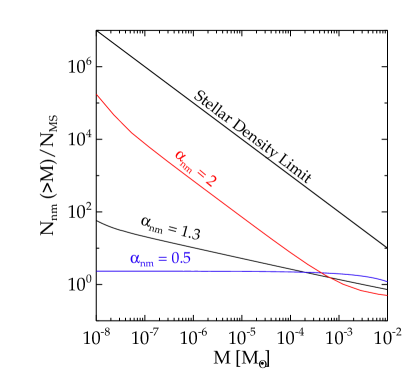
Figure 1.— Number of nomads greater than a given mass scale, $N_{nm}(>M)$, relative to the number of main sequence stars, $N_{\mathrm{MS}}$. Three different slopes for the nomad mass function are labeled, $\alpha_{\mathrm{nm}}=2,1.3,0.5$. The upper black curve is determined assuming that objects at that mass scale have a density of $\rho_{0}=0.1M_{\odot}$ pc^-3.

3. Event Rates

In this section we calculate the microlensing event rates from the nomad population. We begin by establishing the definitions and the Galactic model parameters, and then use this model to predict the timescale distribution of events and the integrated number of events detectable.

3.1. Definitions

We employ standard microlensing formalism. The distance to the source star is $D_{S}$, the distance to the lens is $D_{L}$, and the mass of the lens is $M$. The Einstein radius is $R_{E}^{2}=(4G/c^{2})MD_{L}(D_{S}-D_{L})/D_{S}$, and the Einstein crossing timescale is $t_{E}=R_{E}/v$. The amplification of a source star is $A(u)=(u^{2}+2)/(u\sqrt{u^{2}+4})$, where $u$ is the projected separation of the lens and source in units of the Einstein radius.

To calculate microlensing event rates we use Galactic model 1 of Rahal et al. (2009). This is characterized by an exponential thin disk with a scale length of $R_{d}=3.5$ kpc and scaleheight of $z_{h}=0.325$ kpc,

$$\rho_{d}(R)=\rho_{0}\exp\left[-(R-R_{0})/R_{d}-|z|/z_{h}\right],$$ (1)

where $R_{0}=8.5$ kpc, z_h = 0.35 kpc. We use the bulge density distribution from Dwek et al. (1995). The lens-source transverse velocity distribution, $f(v_{l},v_{b})$ is modeled as in Han & Gould (1996), with $v=\sqrt{v_{l}^{2}+v_{b}^{2}}$, where we indicate as $v_{l}$ and $v_{b}$, respectively, the velocity along the galactic longitude and latitude coordinates.

We determine the total event rate distribution by breaking the lenses-sources into the disk-bulge, bulge-bulge, and disk-disk components. We consider two different targets of source stars. First, bulge stars in the direction of Baade’s window, $(b,l)=(-3.9^{\circ},1^{\circ})$, and second, sources distributed over all-sky. For the bulge observations we can compare to observational determinations of the optical depth (Sumi et al. 2003; Popowski et al. 2005; Sumi et al. 2006; Hamadache et al. 2006) and to the theoretical optical depth calculations (Han & Gould 2003; Wood & Mao 2005) by smoothly extrapolating the rates from the nomad mass regime to the mass regime of main sequence stars and remnants.

3.2. Finite source effects

Since we extrapolate the nomad mass function down to low mass scale, it is important to properly account for finite source effects in the microlensing events. More specifically, we need to estimate by how much the peak amplification of an event is reduced when $R_{E}$ is of order the projected radius of the source star. To estimate finite source effects we take the source stars to have uniform surface brightness, and for a given projected lens-source separation we estimate the amplification as

$$A_{\mathrm{fs}}(u)=\int_{0}^{2\pi}\int_{0}^{\rho_{\star}}d\phi\,\rho d\rho A(\sqrt{u^{2}+\rho^{2}-2u\rho\cos\phi}\,),$$ (2)

where $\rho_{\star}=R_{\odot}/R_{E}$. For typical lens and source distances, $D_{L}\simeq 5$ kpc and $D_{S}\simeq 8$ kpc, and assuming a lens mass $M=10^{-8}M_{\odot}$, the peak amplification is $A_{\mathrm{fs}}\simeq 1.1$. Though this is less than the standard point lens-point mass amplification by $\sim 15\%$, surveys that we consider below will still be sensitive to brightness fluctuations of this magnitude. Extrapolating further down to $M=10^{-9}M_{\odot}$, the peak amplification is only $A_{\mathrm{fs}}\simeq 1.01$. Though extraction of events at this brightness may still be detectable, to provide conservative estimates we restrict our analysis to lens masses $\geq 10^{-8}M_{\odot}$.

3.3. Bulge event rate

The microlensing event rate per source star in a direction $(b,l)$ is given by an integral over the lens-source transverse velocity distribution, the lens density distributions $\rho_{L}$ and the mass function (Griest 1991; Kiraga & Paczynski 1994),

$$\frac{d\Gamma(b,l)}{dt_{E}} = u_{T}\int_{0}^{D_{S}}dD_{L}\int dv_{l}dv_{b}vf(v_{b},v_{l})\delta(t_{E}-R_{E}/v)$$ (3)

$$\times \int_{m_{\mathrm{min}}}^{\infty}dM\zeta(M)R_{E}\rho_{L}(l,b,D_{L}).$$

The mass function $\zeta(M)$ is normalized to the mean mass of the lens population. The optical depth is $\tau\simeq\pi\Gamma/2$, where $\Gamma$ is the integral of the event rate distribution over all $t_{E}$. In Eq. 3, $u_{T}=(A^{2}/\sqrt{A^{2}-1}-1)^{1/2}$, with $A=1.34$ corresponding to $u_{T}=1$. This corresponds to the event rate for source stars within a circular area of one Einstein radius of the lens star. This is a conservative criteria that is appropriate for our analysis; event rates are increased for $u_{T}>1$ when allowing for $A<1.34$.

Figure 2 shows the event rate distributions in the direction of the bulge, with each panel corresponding to a different assumption for the slope of the nomad mass function. In all panels we take $\alpha_{1}=2.0$ and $\alpha_{2}=1.3$ for the main sequence stellar mass function. Within each of the panels there are three different assumptions for $m_{\mathrm{min}}$. The three curves in all of the panels represent the sum of the event rate distribution from bulge and disk lenses. For all curves in the middle and right panels, the mean timescale of a microlensing event is $\langle t_{E}\rangle\simeq 50$ days. However, for the curves in the left panel, $\langle t_{E}\rangle$ depends strongly on $m_{\mathrm{min}}$ because of the steep power law to low masses. Specifically for $m_{\mathrm{min}}=(10^{-2},10^{-5},10^{-8})M_{\odot}$, the respective mean timescales are $\langle t_{E}\rangle\simeq(50,35,3)$ days. For all curves, the optical depths are $\sim 1.5\times 10^{-6}$, consistent with the theoretical calculations above and the observations. The inclusion of the nomad population does not affect the total optical depth because this quantity is independent of the mean mass of the lens population.

Figure 2.— The event rate timescale distribution for several mass functions and cut-off masses. In all panels the solid, dotted, and dashed curves assume $m_{\mathrm{min}}=10^{-2},10^{-5},10^{-8}M_{\odot}$, respectively. The slopes of the mass function in the planetary mass regime ($\alpha_{\mathrm{nm}}$) are indicated in each of the panels.

3.4. All-sky event rate

We now move on to examining the all-sky event rate distribution. In addition to the ingredients input into Eq. 3, here we require two additional pieces of information: the luminosity function of sources, $\phi(m)$, where $m$ is the source apparent magnitude, and the radial distribution of sources $n_{S}(r)$. For the former we use the solar neighborhood $V$-band luminosity function as compiled in Binney & Merrifield (1998), and the $V$-band dust extinction model for the Galaxy as parameterized in Belokurov & Evans (2002). For the latter, we scale the disk density profile by the local density $\rho_{0}$, i.e. $n_{S}=\rho_{d}/\rho_{0}$. Note that here we exclude bulge sources because they only have a few percent contribution to the all-sky microlensing event rate.

With the definitions above, the total microlensing event rate brighter than a limiting magnitude, $m_{\mathrm{lim}}$, is

$$\Gamma(<m_{\mathrm{lim}}) = u_{T}\int_{0}^{m_{\rm lim}}\phi(m)\,dm\int_{0}^{\infty}dD_{S}D_{S}^{2}n_{S}(l,b,D_{L})$$ (4)

$$\times \int_{0}^{D_{S}}dD_{L}\int dv_{l}dv_{b}vf(v_{b},v_{l})$$

$$\times \int_{m_{\mathrm{min}}}^{\infty}dM\zeta(M)\int R_{E}\rho_{L}(l,b,D_{L})\,.$$

Figure 3 shows the integrated all-sky event rate as a function of the limiting magnitude, for the same sets of nomad and brown dwarf mass function parameters that are shown in Figure 2. Here we have included only the event rate for 30 minutes $<t_{E}<$ 1 day. The lower bound for this timescale distribution is motivated by considering the mean timescale for an object of mass $10^{-8}M_{\odot}$, while the upper bound is motivated from Fig. 2, which shows that events from objects with mass $<10^{-2}M_{\odot}$ predominantly have timescales $\lesssim 1$ day. We will further motivate the lower cut-off of 30 minutes when we discuss analysis of observational prospects below. For each curve, the value of $m_{\mathrm{min}}$ is indicated. As Figure 3 shows, there is $\sim 4$ orders of magnitude uncertainty in the predicted nomad event rate brighter than 20th magnitude. For the most shallow allowable nomad mass function, $\alpha_{\mathrm{nm}}=0.5$, the event rate in this range of timescales is $\sim 0.2$ per year, while for the steepest allowable mass function, $\alpha_{\mathrm{nm}}=2$, the event rate is $\gtrsim 10^{3}$ per year.

We note that, when restricting to lens masses $\gtrsim 10^{-2}M_{\odot}$, the event rates determined in Fig. 3 are consistent with prior estimates of $\sim$ few per year for $V<15$ (Nemiroff 1998; Han 2008). Including the entire population of nomads, stars, and remnants, in fact we estimate $\sim 2500$ photometric microlensing events for sources greater than 20th magnitude. Again the vast majority of these events are from disk sources from the high density region towards the Galactic center, with a few percent contribution from bulge sources. The challenge for future observations will clearly be to achieve the appropriate efficiency to extract these short timescale events.

4. Forecast Methodology

The results from the section above provide an estimate of the nomad event rate, independent of the survey specification. In this section, we use the above predictions to estimate how well the nomad population can be measured, given some basic input variables for a survey.

As a general strategy, we would like to determine the constraints on $\alpha_{\mathrm{nm}}$, $\alpha_{\mathrm{bd}}$ and $m_{\mathrm{min}}$ likely to be available from surveys of varying cadence, exposure, and sky coverage. Here we define the exposure in a standard manner as the number of stars monitored, $N_{\star}$, during an observational time period, $T_{\mathrm{obs}}$. For the given exposure and the Galactic model discussed above, we take the data as the observed timescale distributions for a set of microlensing events. We assume that there are $n$ bins distributed over the range of observed $t_{E}$. The minimum and maximum detectable timescale for a survey is set by the detection efficiency, which we estimate below for surveys of different cadence and exposure.

We denote $\Gamma_{\imath}$ as the mean event rate in the $\imath^{th}$ $t_{E}$ bin for a specified exposure, where $\Gamma_{\imath}$ is a function of the model parameters $\alpha_{\mathrm{nm}}$, $\alpha_{\mathrm{bd}}$ and $m_{\mathrm{min}}$. Our goal is to estimate how well we can measure these parameters for an observed event rate distribution. All of the other parameters, such as the local stellar density, the disk scale length and scale height, the bulge mass distribution, and stellar mass function in the regime of main sequence stars and above are fixed to their fiducial values. We do this primarily for simplicity in order to effectively isolate the impact of the nomad population. We assume that the probability for obtaining $N_{\imath}$ events in the $\imath^{th}$ timescale bin follows a Poisson distribution with a mean $\mu_{\imath}=T_{\mathrm{obs}}N_{\star}\Gamma_{\imath}$. For the assumptions above, we can define the elements of the inverse covariance matrix as

$$F_{ab}=\sum_{\imath=1}^{n}\frac{T_{\mathrm{obs}}N_{\star}}{\Gamma_{\imath}}\frac{\partial\Gamma_{\imath}}{\partial\theta_{a}}\frac{\partial\Gamma_{\imath}}{\partial\theta_{b}},$$ (5)

where the indices $a$ and $b$ represent the model parameters, which in our case are $\alpha_{\mathrm{nm}}$, $\alpha_{\mathrm{bd}}$, and $m_{\mathrm{min}}$. From Eq. 5, the one-sigma uncertainty on parameter $a$ is ${\bf F}_{aa}^{-1}$, evaluated at the fiducial values for the parameters. To evaluate Eq. 5 we choose the number of bins $n$ to be equally spaced in log intervals. The main constraint on the bin size will be to ensure that they are wide enough to accommodate a 50% uncertainty in the reconstructed $t_{E}$.

5. Detection Efficiency

In the analysis above, we assumed 100% efficiency when detecting nomads over the entire range of event timescales. In order to obtain a more realistic event rate for a specific survey, we must gain an understanding of how the detection efficiency scales as a function of event timescale. In this section, we describe the basic set-up for our efficiency simulations, and how they are adapted to specific surveys in the sections that follow.

We estimate the detection efficiency via a basic procedure for generating microlensing events. We begin by drawing source and lens objects from the appropriate disk or bulge density distribution. The relative transverse velocity is then drawn from the velocity distribution (Han & Gould 1996). We draw the impact parameter for the source and lens randomly on a uniform interval out to the Einstein radius, and the peak timescale of the event, $t_{0}$, uniformly during the duration of a given survey, $T_{obs}$.

The above set of parameters, $(D_{S},D_{L},v,t_{0})$, along with the event timescale $t_{E}$ fully describe the microlensing event. For this set of parameters, we compute the amplification of the source as a function of time, which by definition peaks at $t_{0}$. The amplification is calculated at time-steps specified by the cadence of the survey. Motivated by the two different survey set-ups that we discuss below, we consider two different models for the survey cadence. First, we consider a uniform cadence model in which the number of time-steps is simply $T_{obs}/t_{\mathrm{cad}}$, where $t_{\mathrm{cad}}$ is the cadence of the survey. Second, we consider a quasi-uniform cadence, in which there are a total of $n_{e}$ epochs for the survey, and $n_{m}$ measurements uniformly spaced per epoch. As discussed below this is most relevant when discussing results for the Gaia survey.

For each point on the lightcurve, the error is estimated from the expected photometric precision. Since the focus of our analysis is on bright microlensing events, we take the error to be uniform for all source stars, and characteristic of the survey that is considered. We then simulate a lightcurve point by sampling from a normal distribution centered on the true point with a variance given by the photometric error. The specific error assumed for each survey will be provided below.

With the above procedure in place, it remains to quantify a criteria for detection for a microlensing event; we choose a relatively simple one that is appropriate for the scope of this work. For our primary analysis we demand that three consecutive points on the lightcurve are $>3\sigma$ deviations from the mean baseline magnitude of a star. This has been used in previous studies (Griest et al. 2011), and provides a good approximation to the criteria discussed in Sumi et al. (2011). The detection efficiency for an input timescale is then the ratio of the number of simulated events that pass the selection criteria to the total number of simulated events at the input timescale.

Figure 3.— Event rate for sources brighter than a limiting magnitude, for different assumed mass functions and cadences. Left panel assumes the nomad and brown dwarf mass function is described by $\alpha_{\mathrm{nm}}=2$ and $\alpha_{\mathrm{bd}}=0$; middle panel assumes $\alpha_{\mathrm{nm}}=1.3$ and $\alpha_{\mathrm{bd}}=0.48$; right panel assumes $\alpha_{\mathrm{nm}}=0.5$ and $\alpha_{\mathrm{bd}}=1.0$. In each panel, the event rate is integrated between timescales of $30$ minutes $<t_{E}<1$ day, and the value of $m_{\mathrm{min}}$ for each curve is indicated in the upper right panel.

6. Projections and Constraints for Specific Surveys

With the above ingredients in place, we now move on to discussing event rates and constraints for specific surveys. We begin by examining next-generation bulge surveys with WFIRST, and then move on to discuss forthcoming all sky surveys Gaia and LSST. We conclude by examining the detection prospects in the short term for the Kepler satellite.

6.1. WFIRST

We first consider the case of a dedicated survey to monitor the inner Galaxy region. This is similar in spirit to the modern MOA, OGLE, and EROS surveys, and to a larger scale, space-based extension such as the proposed WFIRST mission (Green et al. 2011). For the former set of surveys, we can directly use their published detection efficiencies to predict the event rates and model the error distributions, while for a WFIRST type mission this requires simulating events as described above.

For WFIRST, we use a cadence of 15 minutes, a total exposure time of 1 year, and photometric errors of $0.1\%$, which will be achievable down to $J=20.5$. Using the above model, at $t_{E}\sim 0.03$ days we find a detection efficiency of $\sim 50\%$. This high efficiency at short timescale is primarily driven by the order of magnitude increase in the photometric precision relative to modern microlensing experiments. We note that if we assume the MOA-II cadence and photometric uncertainty in their high cadence fields, which we approximate as $\sim 30$ observations per night at $\sim 15$ minute cadence, at $t_{E}=(0.5,1,10)$ days, we find efficiencies of $(10,20,40)\%$, which provides a good approximation to the efficiencies reported in Sumi et al. (2011).

In Figure 4 we show the resulting one- and two-sigma uncertainties on the combination $\alpha_{\mathrm{nm}}$-$\alpha_{\mathrm{bd}}$, for modern and for future dedicated surveys. Here we have assumed fiducial values of $\alpha_{\mathrm{bd}}=0.48$ and $\alpha_{\mathrm{nm}}=1.3$, though we generally find that our results are insensitive to the specific value for these quantities. In plotting the unfilled contours in the left panel, we have assumed an exposure and detection efficiency similar to the MOA-II analysis, which provides a total of $\sim 500$ events for 2 years of observations of 50 million stars; we have assumed $n=20$ bins distributed uniformly in log between timescales of 1-200 days. In this case the errors from our model are in good agreements with the one-sigma uncertainties on $\alpha_{\mathrm{bd}}$ and $\alpha_{\mathrm{nm}}$ presented in Sumi et al. (2011), with slight departures due to the non-gaussian behavior in the tails of the results from the later. In this case the one-sigma errors are $\sigma_{\alpha_{\mathrm{bd}}}\simeq 0.30$ and $\sigma_{\alpha_{\mathrm{nm}}}\simeq 0.40$.

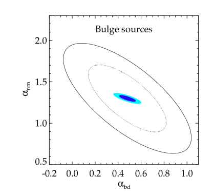
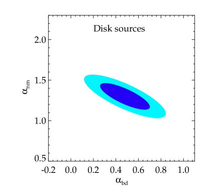
Figure 4.— Left Panel: Joint constraints on the slope of the mass function in the nomad region, $\alpha_{\mathrm{nm}}$, and the slope in the low mass stellar regime, $\alpha_{\mathrm{bd}}$ for bulge sources. Unfilled contours assume the exposure and efficiency of modern bulge surveys, and match the results from Sumi et al. (2011). Inner contour is 68% c.l. and outer contour is 95% c.l. Filled contours are the projected constraints for an exposure and efficiency expected for WFIRST. Right panel: Similar to filled contours on the left, except assuming disk sources.

The filled set of contours in the left panel of Figure 4 show the projected constraints assuming a cadence of 15 minutes and $2\times 10^{8}$ monitored stars for one year. This cadence and exposure is motivated by the preliminary specifications for WFIRST (Bennett et al. 2010). To provide the most optimistic predictions, and as motivated by the photometric precision and the simulations described above, here we have assumed a 100% detection efficiency at all $t_{E}>0.04$ days. In this case, the one-sigma uncertainties are reduced to $\sigma_{\alpha_{\mathrm{nm}}}=0.03$ and $\sigma_{\alpha_{\mathrm{bd}}}\simeq 0.05$, representing nearly an order of magnitude improvement relative to the modern constraints. If we assume $m_{\mathrm{min}}=10^{-3}M_{\odot}$, this corresponds to a measurement of $\beta$ to $\sim 13\%$ precision, and for $m_{\mathrm{min}}=3\times 10^{-7}M_{\odot}$ we have a measurement of $\beta$ to $\sim 25\%$ precision.

For comparison to the bulge results, in the right panel of Figure 4 we show the resulting constraints for disk observations towards $(-2.4^{\circ},331^{\circ})$. This direction is specifically chosen to compare to the results of Rahal et al. (2009). In this case, the constraints on the combination $\alpha_{\mathrm{nm}}$-$\alpha_{\mathrm{bd}}$ are $\sim 3$ times weaker primarily because in this direction only disk lenses are contributing to the event rate.

How well can we determine the minimum mass of a nomad, $m_{\mathrm{min}}$, from a WFIRST type survey? Because a given mass nomad will produce events over a fixed range of timescales (for an assumed velocity distribution function) the answer to this question depends on the value of $m_{\mathrm{min}}$ itself. If the mean event timescale at a given $m_{\mathrm{min}}$ is significantly less than the cadence of the survey, then observations will not effectively be able to probe this mass scale.

In Figure 5 we show the resulting fractional uncertainty on $m_{\mathrm{min}}$ for a cadence of 15 minutes and bulge observations. In this case, for $m_{\mathrm{min}}\gtrsim 10^{-5}M_{\odot}$ we find fractional uncertainty $\gtrsim 30\%$. In fact down below the Earth mass scale for $m_{\mathrm{min}}\gtrsim 10^{-6}M_{\odot}$ we still find fractional uncertainty $\sim 50\%$, below which there is degradation of the constraints because the event rate in the observable timescale window becomes too low.

Figure 5.— Fractional uncertainty on $m_{\mathrm{min}}$ for a cadence of 15 minutes and bulge observations.

6.2. Large-Scale Surveys: Gaia and LSST

We now extend to consider projected constraints on $\alpha_{\mathrm{nm}}$-$\alpha_{\mathrm{bd}}$ from all-sky observations. In this case, estimating the detection efficiency of the survey will be crucial in order to understand what fraction of the total event rate shown in Figure 3 will be accessible.

The two primary templates we consider for large scale surveys are those being planned for Gaia and LSST. These multi-purpose surveys are not expected to have cadence as high as the dedicated inner Galaxy observations discussed above, so they will not be as sensitive to very short timescale microlensing events. However by their nature all-sky observations do probe the nomad population on a Galaxy-scale that are inaccessible to dedicated pointings towards a fixed region of the Galaxy.

6.2.1 Gaia

As our first example of a survey with a non-uniform cadence, we consider Gaia, which is scheduled to launch in 2013. Though Gaia is primarily designed as an astrometric mission, it will have a single measurement photometric accuracy of $\sim 10$ mmag for sources brighter than its broadband 20th magnitude. Because of the Gaia scanning strategy, the sampling for each star is not uniform during the mission lifetime. Measurements will be grouped into epochs, during which an observation is performed in $\sim 6$ hr intervals. The mean number of measurements per epoch is $\sim 5$, though some epochs will have a minimum of $7$ measurements  (Eyer & Mignard 2005). The mean number of visits between epochs is 25-35 days, though depending on Galactic latitude we estimate from the results of Eyer & Mignard (2005) that $\sim 10\%$ of the stars will have $\sim 5$ days between epochs.

Motivated by these specifications, we model Gaia observations by considering a quasi-irregular sampling pattern. For the baseline model we assume 25 days between epochs, and within each epoch there are five photometric measurements. This is the approximate mean sampling rate of Gaia (Eyer & Mignard 2005). The survey is run for a total of $T_{obs}=5$ years, resulting in a mean of 300-400 photometric samples for the lifetime of the survey. To model the distribution of disk sources we use the $V$-band luminosity function described above, along with the Belokurov & Evans (2002) dust extinction parameterization.

For a Gaia-like sampling, the short timescale events, $t_{E}\sim 1$ day, will occur during an epoch, and it is possible that a peak of the microlensing event will not be discernible. To account for this, we modify the detection criteria. For a simulated event at an input timescale, we again search for three points on the lightcurve that are greater than 3-$\sigma$ deviations from the baseline magnitude of the source. In addition we include a second, stricter cut to the detection criteria, namely that the peak of the event is observable.

Given the above algorithm, for the Gaia sampling pattern, at $t_{E}=1$ day we find a detection efficiency of $1\%$.

For the Gaia cadence and estimated efficiency, in Figure 6 we show the joint constraints on $\alpha_{\mathrm{nm}}$ and $\alpha_{\mathrm{bd}}$ for all-sky observations. Here we have assumed a five year lifetime of the mission. In this case the constraints are similar to the current constraints on these parameters because of the similar event rates after our detection efficiency cuts have been implemented.

6.2.2 LSST

As our second example, we examine the somewhat deeper survey we anticipate being carried out by the LSST. This system will repeatedly survey the entire visible southern sky to a $5$-sigma point source depth of $g=25.0$, $r=24.7$ per epoch. LSST is expected to have a mean cadence (across all filters) of less than 4 days and a mission lifetime of 10 years (LSST Science Collaborations et al. 2009). To achieve a synoptic survey, the LSST will follow a logarithmic sampling pattern, with 15-second exposures separated by 15 seconds, 30 minutes, 3–4 days and one year, with considerable scatter in the two intermediate cadences to allow flexible scheduling. Two back-to-back exposures constitute a “visit”; the baseline plan has each field being visited twice on any of its observation nights. As with Gaia, detection of a nomad by microlensing requires seeing both sides of a peak in the lightcurve, suggesting that events with timescales less than 3 days may be difficult to detect.

To approximate the sampling strategy of LSST, we assume a uniform cadence for the lifetime of the survey. From the formalism above we have calculated the detection efficiency for cadences of both 1 and 4 days; we consider higher cadence dedicated campaigns with LSST below. We find that only for a 1 day cadence is it possible to achieve 1% detection efficiency for timescales $t_{E}\gtrsim 1$ day. For a 4-day cadence, the efficiency for detecting nomads drastically drops (though in this case a large number of brown dwarf events will still be measured very precisely). We utilize this optimistic 1% efficiency when we calculate the projected constraints on $\alpha_{\mathrm{nm}}$-$\alpha_{\mathrm{bd}}$ for the uniform cadence model.

To model the distribution of sources for our LSST predictions we use the $I$-band luminosity function from Zheng et al. (2004). In this case, dust extinction modeled by adopted in the model of Belokurov & Evans (2002) and scaling according to the standard extinction law between wavebands (Rieke & Lebofsky 1985).

The left panel of Figure 6 shows the results of the analysis. As indicated, the constraints are weaker relative to the left panel; this is mainly due to the reduced efficiency as compared to the Gaia sampling model.

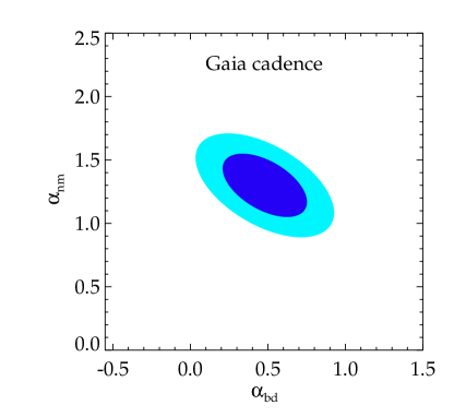
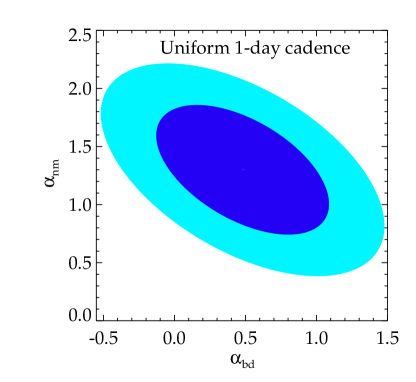
Figure 6.— Joint constraints on $\alpha_{\mathrm{nm}}$ and $\alpha_{\mathrm{bd}}$ for all-sky observations. The left panel shows results for the irregular sampling pattern that represents the Gaia mission, while the right panel represents the uniform sampling pattern that may be achievable with LSST.

6.3. Kepler

As our final example we study the nomad event rate measurable by the Kepler satellite. Kepler monitors $\sim 100$ deg² towards the Cygnus region, and has a photometric precision of approximately 80 ppm for sources brighter than $V=13$, and a few percent for sources at $V=20$. Kepler is complete down to $V=17$. The integration time is 30 minutes for the majority of Kepler sources. For $\alpha_{\mathrm{nm}}=2$ and $m_{\mathrm{min}}=10^{-8}M_{\odot}$, and assuming $m_{\mathrm{min}}=10^{-8}$ down to 20th magnitude, the raw event rate is a few per year for 30 minutes $<t_{E}<$ 1 day. For $\alpha_{\mathrm{nm}}<2$ we find less than one event per year. However, these predictions are for $u_{T}=1$; due to its precise photometry of $\sim 80$ ppm for bright stars with $V<13$ the event rate is proportionally larger for $u_{T}>1$. Thus discovery of anomalous microlensing events in the Kepler data may indicate a steep value for the nomad mass function, and warrant a dedicated analysis of the photometry of Kepler stars.

7. Detecting Short Timescale Events

In the above analysis we have restricted only to events with timescales sufficiently long to be detectable according to the criteria above. What if we relax this criteria, and expand to consider events with shorter timescales, over which the lightcurves are much more sparsely sampled? Is it still possible to detect microlensing events from lighter nomads over much shorter timescales?

As an example let us consider the planned survey strategy of LSST. In a given LSST filter, each visit will consist of two consecutive 15 second exposures separated by a 4 second readout interval. When possible, each field will be observed twice, with visits separated by $\sim 15-60$ minutes. For stars with $r\lesssim 20$, the single visit photometric precision of each measurement is $\sim 10$ mmag. Though per visit the photometry is very precise and the 30 second cadence is short, two points on a lightcurve are not adequate to claim the detection of a microlensing event. However, the lack of variation of a source star over this timescale in between visits could allow us to bound the existence of nomads with characteristic timescales $\sim 30$ seconds. Assuming both the lenses and the sources to be in the disk, this timescale corresponds to a lens of mass $\lesssim 10^{-10}M_{\odot}$.

Will lenses with such a small mass cause noticeable brightness fluctuations in a star when accounting for finite source effects? For our uniform source surface brightness model, we find that this depends on the lensing geometry. For example, with $D_{L}=1$ kpc and $D_{S}=5$ kpc, a lens of mass $[10^{-9},10^{-10}]M_{\odot}$ will have a peak brightness of $A_{\mathrm{fs}}\simeq[1.01,1.001]$. For lenses nearer to the source, $A_{\mathrm{fs}}$ is reduced from these values. Though these are smaller brightness fluctuations than typically searched for in microlensing events, the presence of these objects may be limited given the photometric precision of LSST.

In perhaps more near of a term, we may entertain the prospect of a dedicated telescope that is capable of detecting short timescale microlensing events that last for as little as tens of seconds. As an example, we will consider a liquid mirror telescope similar in design to the six-meter Large Zenith Telescope  , only in our case positioned in the Southern hemisphere to cover the Galactic bulge. For a $4000\times 4000$ CCD chip with $1^{{}^{\prime\prime}}$ per pixel and a 6-m aperture, in less than a day a patch of area $\sim 100$ square degrees could be scanned. We focus on the $I$-band, and take the bulge as an example with an surface brightness of $17.6$ mag arcsec^-2 (Terndrup 1988). Assuming that the signal-to-noise is dominated by the unresolved light from the bulge and shot noise, for a star with $I=19$ the signal-to-noise is $S/N\simeq 37\sqrt{t/{\rm sec}}$. A 10-second exposure then gives a photometric precision of $\sim 1\%$, and during this time a star crosses through $\sim 10^{3}$ pixels. This would likely be sufficient to obtain several points on a lightcurve to measure a microlensing event with $t_{E}\sim 30$. sec.

For a nomad mass function of $dN/dM\sim M^{-2}$ with $m_{\mathrm{min}}=10^{-9}M_{\odot}$, for a 100 deg² patch that passes through the Galactic center we find $\sim 50$ events per year with $t_{E}>30$ seconds for source stars with $I<19$. The event rate may even be up to an order of magnitude larger for steeper values of the mass function over the range $10^{-9}M_{\odot}$. It is also worthwhile to point out that a telescope designed along these lines could also be a relatively inexpensive endeavor. Further, a liquid mirror telescope with mercury could extend to the near-infrared, where the reflectivity would be similar to that in the optical.

8. Discussion and Conclusions

We have estimated that there may be up to about $10^{5}$ compact objects per main sequence star in the Galaxy that are greater than the mass of Pluto. A dedicated high cadence survey of the inner Galaxy, such as would be possible with WFIRST, could measure the number of nomads greater than the mass of Jupiter per main sequence star to $\sim 13\%$ , and the corresponding number greater than the mass of Mars to $\sim 25\%$. Also WFIRST can measure the minimum mass of the nomad population to about 30%. Large-scale surveys, in particular that of Gaia, could identify nomads in the Galactic disk that are greater than about the mass of Jupiter.

Observations along the lines that we discuss will constrain the nomad population of the disk relative to the bulge, and will also more generally improve the star-star microlensing event rate in the disk and the solar neighborhood, about which very little is now known (Gaudi et al. 2008; Fukui et al. 2007; Rahal et al. 2009). Further, they will improve our understanding of the mass function of low mass brown dwarfs and super-Jupiters, and the distinction between these classes of objects (Spiegel et al. 2011).

How will these measurements compare to modern microlensing measurements of low mass brown dwarf population from disk observations? To answer this question we can briefly consider the results from Rahal et al. (2009). These authors find a total of $\sim 20$ events in three fields in which the lenses are primarily disk sources, and in particular there are two very short timescale lenses, at $t_{E}=7$ and $12$ days. While the data are not sufficient at present to perform a full statistical analysis and constrain $\alpha_{\mathrm{nm}}$ and $\alpha_{\mathrm{bd}}$, from an analysis of these data one may deduce that a steeper model brown dwarf mass function is favored over a more shallow model. The inclusion of the nomad population does mildly improve the statistical fit, though in order to probe this population with disk observations a survey must build up a sufficient event rate in the $\sim 1-10$ day timescale bin.

How will the future microlensing measurements we discuss compare to direct measurements of the brown dwarf mass function? Metchev et al. (2007) find that for warm brown dwarfs the mass function may be flat, $\alpha_{\mathrm{bd}}=0$. For cooler brown dwarfs the recent WISE observations are consistent with a wide range of $\alpha_{\mathrm{bd}}$ between $0-1$ (Kirkpatrick et al. 2011). Other microlensing observations shed light on the brown dwarf mass function, though they do not clarify the picture. For example, Gould et al. (2009) uncover an extreme magnification microlensing event and interpret it as due to a thick disk brown dwarf. According to  Gould et al. (2009), there is a very low probability to observe this event given our standard population of brown dwarfs in the Galactic disk given the large velocity of the event. The existence of these events either implies that we have been lucky to observe events at all (in particular with the large observed magnifications), or that the local population of low mass and low luminosity stellar remnants is larger than is presently predicted.

If a nomad is identified via the methods described in this paper, there are a number of follow-up observations that are possible. For example even though Gaia will only do on average 1-2 one-dimensional astrometric measurements per epoch, it may be possible to confirm the photometric detection with astrometry for the brightest sources by comparing the centroid of the source during the event to the baseline centroid as determined over several epochs during the course of the mission.

Finally we note that an additional outcome of the observational approach discussed above, especially regarding the detection of short timescale microlensing events, is that upper limits may be set on the density of nomads. This could set very interesting constraints on the population of planetesimals in nascent planetary systems.

References

- Abbot & Switzer (2011) Abbot, D. S., & Switzer, E. R. 2011, ApJ, 735, L27
- Baumgartner & Mushotzky (2006) Baumgartner, W. H., & Mushotzky, R. F. 2006, Astrophys. J. , 639, 929
- Belokurov & Evans (2002) Belokurov, V., & Evans, N. 2002, Mon.Not.Roy.Astron.Soc., 331, 649
- Bennett et al. (2010) Bennett, D. P., et al. 2010, ArXiv e-prints, 1012.4486
- Bernstein et al. (2004) Bernstein, G. M., Trilling, D. E., Allen, R. L., Brown, M. E., Holman, M., & Malhotra, R. 2004, Astron. J., 128, 1364
- Bihain et al. (2009) Bihain, G., et al. 2009, Astron.&Astrophys, 506, 1169
- Binney & Merrifield (1998) Binney, J., & Merrifield, M. 1998, Galactic Astronomy, ed. Binney, J. & Merrifield, M.
- Borucki et al. (2010) Borucki, W. J., et al. 2010, Science, 327, 977
- Boss (2000) Boss, A. P. 2000, ApJ, 536, L101
- Caballero et al. (2007) Caballero, J. A., et al. 2007, Astron.&Astrophys, 470, 903
- Debes & Sigurdsson (2007) Debes, J. H., & Sigurdsson, S. 2007, ApJ, 668, L167
- Dwek et al. (1995) Dwek, E., Arendt, R., Hauser, M., Kelsall, T., Lisse, C., et al. 1995, Astrophys.J., 445, 716, fermilab Library Only
- Eyer & Mignard (2005) Eyer, L., & Mignard, F. 2005, Mon.Not.Roy.Astron.Soc.
- Francis (2005) Francis, P. J. 2005, Astrophys. J. , 635, 1348
- Fukui et al. (2007) Fukui, A., et al. 2007, Astrophys. J., 670, 423
- Gaudi (2010) Gaudi, B. S. 2010, ArXiv e-prints
- Gaudi et al. (2008) Gaudi, B. S., et al. 2008, Astrophys. J., 677, 1268
- Gould et al. (2009) Gould, A., et al. 2009, Astrophys. J., 698, L147
- Green et al. (2011) Green, J., et al. 2011, ArXiv e-prints, 1108.1374
- Griest (1991) Griest, K. 1991, Astrophys.J., 366, 412
- Griest et al. (2011) Griest, K., Lehner, M. J., Cieplak, A. M., & Jain, B. 2011, ArXiv e-prints, 1109.4975
- Hamadache et al. (2006) Hamadache, C., Le Guillou, L., Tisserand, P., Afonso, C., Albert, J., et al. 2006, Astron.Astrophys., 454, 185
- Han (2008) Han, C. 2008, Astrophys. J. , 681, 806, 0708.1215
- Han & Gould (2003) Han, C., & Gould, A. P. 2003, Astrophys.J., 592, 172
- Han & Gould (1996) Han, C.-h., & Gould, A. 1996, Astrophys.J., 467, 540
- Holmberg & Flynn (2000) Holmberg, J., & Flynn, C. 2000, Mon.Not.Roy.Astron.Soc., 313, 209
- Jayawardhana & Ivanov (2006) Jayawardhana, R., & Ivanov, V. D. 2006, Science, 313, 1279
- Jura (2011) Jura, M. 2011, Astron. J., 141, 155
- Kiraga & Paczynski (1994) Kiraga, M., & Paczynski, B. 1994, Astrophys. J., 430, L101
- Kirkpatrick et al. (2011) Kirkpatrick, J. D., et al. 2011, ApJS, 197, 19
- LSST Science Collaborations et al. (2009) LSST Science Collaborations et al. 2009, ArXiv e-prints, 0912.0201
- Metchev et al. (2007) Metchev, S., Kirkpatrick, J., Berriman, G., & Looper, D. 2007, Astrophys.J.
- Nemiroff (1998) Nemiroff, R. J. 1998, Astrophys. J., 509, 39
- Popowski et al. (2005) Popowski, P., et al. 2005, Astrophys.J., 631, 879
- Rahal et al. (2009) Rahal, Y. R., et al. 2009, Astron. Astrophys., 500, 1027
- Rees (1976) Rees, M. J. 1976, Mon. Not. R. Astron. Soc., 176, 483
- Rieke & Lebofsky (1985) Rieke, G. H., & Lebofsky, M. J. 1985, Astrophys. J., 288, 618
- Spiegel et al. (2011) Spiegel, D. S., Burrows, A., & Milsom, J. A. 2011, Astrophys.J., 727, 57
- Stevenson (1999) Stevenson, D. J. 1999, Nature, 400, 32
- Sumi et al. (2003) Sumi, T., Abe, F., Bond, I., Dodd, R., Hearnshaw, J., et al. 2003, Astrophys.J., 591, 204
- Sumi et al. (2011) Sumi, T., Kamiya, K., Udalski, A., Bennett, D., Bond, I., et al. 2011, Nature, 473, 349
- Sumi et al. (2006) Sumi, T., Wozniak, P., Udalski, A., Szymanski, M., Kubiak, M., et al. 2006, Astrophys.J., 636, 240
- Terndrup (1988) Terndrup, D. M. 1988, Astron. J., 96, 884
- Tisserand et al. (2007) Tisserand, P., et al. 2007, Astron.&Astrophys, 469, 387
- Wolfgang & Laughlin (2011) Wolfgang, A., & Laughlin, G. 2011, ArXiv e-prints
- Wood & Mao (2005) Wood, A., & Mao, S. 2005, Mon.Not.Roy.Astron.Soc., 362, 945
- Zheng et al. (2004) Zheng, Z., Flynn, C., Gould, A., Bahcall, J. N., & Salim, S. 2004, Astrophys.J., 601, 500