Force localization in contracting cell layers

Abstract

Epithelial cell layers on soft elastic substrates or pillar arrays are commonly used as model systems for investigating the role of force in tissue growth, maintenance and repair. Here we show analytically that the experimentally observed localization of traction forces to the periphery of the cell layers does not necessarily imply increased local cell activity, but follows naturally from the elastic problem of a finite-sized contractile layer coupled to an elastic foundation. For homogeneous contractility, the force localization is determined by one dimensionless parameter interpolating between linear and exponential force profiles for the extreme cases of very soft and very stiff substrates, respectively. If contractility is sufficiently increased at the periphery, outward directed displacements can occur at intermediate positions, although the edge itself still retracts. We also show that anisotropic extracellular stiffness leads to force localization in the stiffer direction, as observed experimentally.

Actively generated forces have emerged as a central element in the way tissue cells interact with their environment, for example during development and tissue maintenance Wozniak and Chen (2009). It is becoming increasingly clear that cells use physical force to probe the mechanical properties of their environments and to create a structurally coherent state within the cell and tissue. Experimentally, however, it is challenging to measure cellular forces in a physiological context. Therefore their effect is usually assessed in an indirect manner, for example by mechanical relaxation after laser cutting Hutson et al. (2003).

In order to directly measure the forces that cells exert on their environments, two complementary techniques have been established over the last decade. Embedding marker beads into soft elastic gels enables the measurement of the displacement field generated by cell traction forces applied to the surface of the gel, which can then be estimated using elasticity theory Dembo and Wang (1999). Alternatively, microfabrication techniques are used to create an array of elastomeric pillars, which for small displacements each act as a linear spring Tan et al. (2003).

In order to address the role of forces for larger cell clusters, both soft elastic substrates and pillar assays have been used for confluent layers of epithelial cells. Placing such cells on a pillar array, it was found that cellular traction forces are localized to the edge of the cell layer du Roure et al. (2005); Saez et al. (2010). A qualitatively similar effect has also been observed for cell sheets migrating over soft elastic substrates Trepat et al. (2009), although in this case the length scales over which the stresses decayed were greater. It is tempting to assume that force localization to the edge reflects increased mechanical activity of the cells at the edge, for example of putative leader cells Khalil and Friedl (2010). However, a more detailed analysis requires a mechanical analysis of the cell sheet coupled to the elastic foundation.

In this Letter, we analytically solve the problem of a contracting cell layer coupled to a layer of springs. For homogeneous contraction, we show that the problem is determined by one dimensionless parameter which interpolates between the extreme cases of soft pillars with a linear force profile and stiff pillars with an exponential force profile. We also show how our results change for increased contractile activity at the rim and for substrates with anisotropic stiffness.

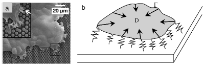
Figure 1: (a) Scanning electron micrographs of an epithelial cell layer on an array of microfabricated elastomeric pillars (image reproduced from du Roure et al. (2005).) (b) A schematic representation of the pillar assay. The cell layer contracts and is resisted by a distribution of linear springs on the surface.

Elastic model. Microstructured surface assays consist of a regular array of flexible elastomeric pillars with defined surface chemistry, see Fig. 1. For small displacements and slender pillars, the relation between the traction applied to the pillars $\mathbf{T}$ and the displacement $\mathbf{u}$ follows from linear elasticity theory Landau and Lifschitz (1986),

$$\mathbf{T} = k\mathbf{u}\,=\,\left(\frac{3\pi}{4}E_{\mathrm{p}}\frac{r^{4}}{L^{3}}\right)\mathbf{u},$$ (1)

where $r$ and $L$ are the radius and height of the pillar, respectively, and $E_{\mathrm{p}}$ is the Young’s modulus. The pillars thus behave as simple linear springs with effective spring constant $k$.

In the assays of interest the substrate is usually coated with adhesion-promoting molecules so that the cells spread thinly and form a confluent layer. We thus assume the layer behaves as a continuous elastic solid. In addition, as the typical lateral extension of the sheet is much larger than the layer thickness $h$, we have the conditions for plane-stress in the layer and can use a two-dimensional model for the cells. The force balance then reads

$$\mathrm{div}\cdot\mathbf{F}-kN\mathbf{u} = \mathbf{0},$$ (2)

where $\mathbf{F}$ is the two-dimensional in-plane stress tensor obtained by averaging the layer stress over the thickness, and $N$ is the number density of pillars. For a continuous elastic substrate, the restorative force applied to the cell layer would not take this simple form. Moreover more detailed assumptions would be required to define the elastic problem of the two coupled elastic layers. Nevertheless, the linear traction force term from Eq. 2 can be also considered as a first order approximation for soft elastic substrates Murray (2003); Edwards and Chapman (2007).

The cell layer is mechanically active, with cells simultaneously repositioning and contracting. Here we consider only the final configuration of a contractile cell layer. Then the problem of modelling layer contraction is similar to that of thermoelasticity, where temperature changes generate expansion or contraction in the material Murray (2003). In thermoelasticity one typically introduces an expansion term proportional to the target volume change into the constitutive relation Landau and Lifschitz (1986). In analogy we take

$$F_{ij}=\frac{hE_{\mathrm{c}}}{1+\nu}\left(e_{ij}+\frac{\nu}{1-\nu}e_{kk}\delta_{ij}\right)-\frac{hE_{\mathrm{c}}}{2(1-\nu)}P\delta_{ij}.$$ (3)

The first term is the usual plane-stress linear elastic constitutive relation with $E_{\mathrm{c}}$ the cellular Young’s modulus, $\nu$ the cellular Poisson’s ratio, and $e_{ij}$ the strain tensor. The second term in Eq. (3) captures cellular contractility, where we have assumed that the contraction is isotropic. If the layer is under no stress, $F_{ij}=0$ and thus $P=e_{ii}$ (summation convention applies), and so $P$ is the local target volume change of a material element in the cell layer.

At the layer boundary no stress is applied, giving the boundary condition $\mathbf{F}\cdot\mathbf{n}=\mathbf{0}$ on $\Gamma$. Integrating Eq. (2) over the cell area $D$ and applying the zero-stress boundary condition gives $\int_{D}kN\mathbf{u}=\mathbf{0}$. Thus momentum is not generated in the system, as expected for a closed system.

Solution for a contracting stripe. It is instructive to first solve our elastic problem in one dimension, although experimentally even very anisotropic cell layers always contract in both lateral directions. We consider a rectangular sheet with $e_{yy}=0$, such that the layer contracts only in the $x$-direction over the stripe width $l_{0}$. Substituting Eq. (3) into Eq. (2) we find that $u(x)$ satisfies

$$\frac{\mathrm{d}^{2}u}{\mathrm{d}x^{2}}-\frac{1}{l^{2}}u \,=\,\frac{1}{2}(1+\nu)\frac{\mathrm{d}P}{\mathrm{d}x}$$ (4)

with the zero stress boundary condition $\mathrm{d}u/\mathrm{d}x=(1+\nu)P/2$ at $x=\pm l_{0}$ and with $u=0$ at $x=0$. Here we have introduced a new length scale, the localization length

$$l=\sqrt{\frac{hE_{\mathrm{c}}}{kN(1-\nu^{2})}}=\sqrt{\frac{4hE_{\mathrm{c}}L^{3}}{3\pi(1-\nu^{2})E_{\mathrm{p}}Nr^{4}}},$$ (5)

with the second expression following from Eq. (1).

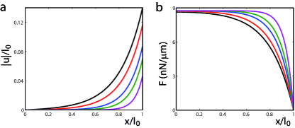
Figure 2: (Color online) Plot of (a) displacement $|u|$ and (b) stress $F$ within the cell layer for the stripe geometry with $P_{0}=0.7$, $E_{\mathrm{c}}=10\,\mathrm{kPa}$, $h=1\,\mu\mathrm{m}$, $\nu=0.45$ and $\gamma=$5, 6, 8, 10, 15 (from top to bottom in (a) and from bottom to top in (b)).

Assuming that the cell layer contracts uniformly, $P$ is constant. For the stripe case, it is convenient to set $P=-2P_{0}/(1+\nu)$ where $P_{0}$ is then the target contraction in the $x$-direction. We then find that Eq. (4) is solved by

$$\frac{u}{l_{0}} = -P_{0}\frac{\mathrm{sinh}(\gamma x/l_{0})}{\gamma\mathrm{cosh}\gamma}$$ (6)

where we have defined the dimensionless localization parameter $\gamma=l_{0}/l$, the ratio of layer dimension to the localization length $l$. The internal stress $F(x)$ can be obtained by substituting Eq. (6) into the constitutive relation Eq. (3), see SI SI .

In Fig. 2 the displacement $u$ and internal stress $F$ are plotted for different values of $\gamma$. We see that a constant cellular contraction leads to non-constant pillar displacement, with greatest deflections at the edge. The non-dimensional parameter $\gamma$ controls the profile of the solution and the rate of decrease of observed tractions away from the layer edge. When $\gamma$ is large, the pillars dominate the system and restrict the displacements to a small region near the rim. When $\gamma$ is small, the substrate resists less and the tractions decay slower. Note that both displacement and stress scale linearly with cell contraction $P_{0}$.

Solution for a contracting disc. We now consider the two-dimensional problem of a circular cell layer with isotropic contraction, which is directly comparable to experiments with finite-sized and isotropically contracting cell layers. From symmetry arguments $\mathbf{u}=u(r)\mathbf{e}_{r}$, where $r$ is the radial distance from the centre of the plate. The radially symmetric equivalent to Eq. (4) reads

$$r^{2}\frac{\mathrm{d}^{2}u}{\mathrm{d}r^{2}}+r\frac{\mathrm{d}u}{\mathrm{d}r}-\left(1+\frac{r^{2}}{l^{2}}\right)u = \frac{1}{2}(1+\nu)r^{2}\frac{\mathrm{d}P}{\mathrm{d}r}.$$ (7)

The boundary conditions are now $u=0$ at $r=0$, while at $r=r_{0}$ we have $P=2(\mathrm{d}u/\mathrm{d}r+u/r)/(1+\nu)$.

Considering again the case of constant cellular contraction, $P=-P_{0}$, the solution of Eq. (7) with the specified boundary conditions can be calculated in terms of modified Bessel functions:

$$\frac{u}{r_{0}} = -\frac{1}{2\gamma}P_{0}(1+\nu)A(\gamma)I_{1}(\gamma r/r_{0}),$$ (8)

$$A(\gamma) = \left(I_{0}(\gamma)+\frac{\nu-1}{\gamma}I_{1}(\gamma)\right)^{-1}.$$ (9)

Again $\gamma=r_{0}/l$ is the ratio of sample dimension and localization length, i.e. the decay length scale for the traction forces $l$. From Eq. (8) the radial stresses $F_{rr}$ and hoop stresses $F_{\theta\theta}$ in the layer can be calculated, see SI SI , which show a similar behaviour as in the one-dimensional case from Fig. 2(b), except that the hoop stress does not vanish at the boundary. The plot for displacement essentially looks like the one for the stripe case, Fig. 2(a), see SI SI . Our results are consistent with the simulations in Mohrdieck et al. (2005), where a uniformly contracting network of actin fibres on a discrete pillar array was also observed to exhibit localisation of force to the edges of the network.

Regarding the comparison with experiments, typical parameter values are $N=0.25\,\mu\mathrm{m}^{-2}$ for the pillar density, $r_{0}=50\,\mu\mathrm{m}$ for layer dimension, $h=1\,\mu\mathrm{m}$ for layer thickness, $E_{\mathrm{c}}=10\,\mathrm{kPa}$ for cellular Young’s modulus and $\nu=0.45$ for Poisson’s ratio. With pillar stiffness ranging over 1 - 200 $\mathrm{nN}\,\mu\mathrm{m}^{-1}$ Saez et al. (2010), this gives a typical range for the dimensionless parameter $\gamma\sim 7-100$. The clear decay of the traction profile reported in Saez et al. (2010) agrees nicely with our results. A more spread-out traction profile has been reported in Trepat et al. (2009), which may be attributable to a low value of $\gamma$. However, as this study focused on the dynamics in a migrating sheet, direct comparison is difficult in this case.

To further examine the role of $\gamma$ in determining the profile of the solution, we consider the limiting cases of $\gamma$ small and large. When $\gamma$ is small, the pillars are very weak and the layer will be able to contract by a large amount. When $\gamma\ll 1$, we obtain to lowest order a linear profile $u\sim-P_{0}r/2$, as one can infer either directly from the differential equation or from the Bessel function. Alternatively, in the case $\gamma\gg 1$, when the springs dominate the behaviour of the sheet, the displacement localizes strongly to the edge and we get an exponential profile,

$$u \sim -\frac{P_{0}r_{0}(1+\nu)}{2\gamma}e^{-\gamma(1-r/r_{0})}.$$ (10)

The exact profile of the solution is thus clearly controlled by the non-dimensional parameter, $\gamma$, which quantifies the relative strengths of pillars versus cells.

Effect of a contractile rim. Up to now, we have assumed that the layer undergoes a uniform contraction. We now apply our model for the contractile cell layer to two further situations of large practical interest, namely non-homogeneous contraction in the layer and anisotropic layer stiffness. We first consider what the displacements would look like if the layer had a more mechanically active rim. We consider that the contraction jumps up at the rim:

$$P=\left\{\begin{array}[]{l l}-P_{0}&\quad\text{$x<x_{1}$ or $r\leq r_{1}$ }\\ -P_{1}&\quad\text{$x_{1}<x<l_{0}$ or $r_{1}<r<r_{0}$}\\ \end{array}\right.,$$ (11)

for both the contracting stripe and disc. Eqs. (4) and (7) are unchanged, as are the boundary conditions applied at both the origin ($u=0$) and edge of the layer (zero normal stress). At the interface between the two contractile regions (i.e. at $x=x_{1}$ and $r=r_{1}$, for the stripe and disc case, respectively), however, we impose the additional conditions that the displacement $u$ and stresses $F$ (for stripes) and $F_{rr}$ (for discs) are continuous across the interface. With these additional boundary conditions it is possible to obtain analytical solutions for the displacement $u$, see SI SI .

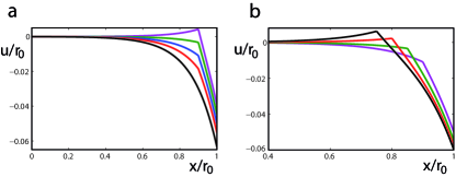
Figure 3: (Color online) Plot of displacement $u$ in a disc with contractile rim for (a) $P_{0}/P_{1}=$0.1, 0.3, 0.5, 0.7, 1 with $r_{1}/r_{0}=0.9$ (from top to bottom), (b) $r_{1}/r_{0}=$0.75, 0.8, 0.85, 0.9, with $P_{0}/P_{1}=0.5$ (from top to bottom). In both plots $\gamma=8$, $P_{1}=0.7$, $\nu=0.45$.

For the disc geometry, the resulting displacement is plotted in Fig. 3(a). Note that the plot of the displacement $u$ has a kink at the point of transition between the two contractilities, and that as the inner region becomes weaker and $P_{0}/P_{1}$ decreases, this feature is accentuated. Equally, as $P_{0}/P_{1}\to 1$, this feature disappears and we recover the solution for constant contractility. The displacements for the contracting stripe solution are qualitatively the same.

For a sufficiently inactive inner region, there is the possibility that contraction of the outer rim dominates to such an extent that it can pull the inner region towards it, resulting in positive displacements at intermediate positions, although the layer as a whole retracts its edge. This effect depends sensitively on the spatial extent of the contracile rim. For the stripe case with $x_{1}/x_{0}=1-\epsilon$ and $\epsilon\ll 1$, positive displacements are possible only when $P_{0}\sim\epsilon^{2}\gamma^{2}P_{1}/2$, see SI SI . This dependence on the extent of the more contractile region is also seen in Fig. 3(b). In summary, the existence of kinks and positive displacements in experiments would be a clear signature of increased contractility at the rim.

Solution for anisotropic pillars. In a natural setting, cells are often confronted with highly anisotropic environments, which can have a strong effect on their response. This important effect can be investigated experimentally by using pillars with elliptical cross-sections Tan et al. (2003); Saez et al. (2007, 2010). Then the apparent stiffness of the substrate depends on the direction,

$$k(\theta)=K\left(1+\epsilon\cos^{2}\theta\right),$$ (12)

where $\theta$ is defined to be the angle of the pillar deflection with respect to the major axis $a$. The minor axis is given by the relation $a^{2}=b^{2}(1+\epsilon)$. The spring constant is now $K=3\pi E_{\mathrm{p}}b^{3}a/4L^{3}$ and so we redefine $\gamma^{2}=r_{0}^{2}KN(1-\nu^{2})/hE_{\mathrm{c}}$. Using these arrays it is observed in Saez et al. (2007, 2010) that tissues elongate along the major axes of the pillars, with cellular force being concentrated at the pointed ends of the layers.

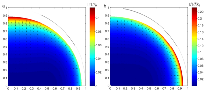
Figure 4: (Color online) Plot of (a) displacement $|u|$, arrows indicate displacement directions and magnitude, (b) traction force $f/Kr_{0}$ exerted on pillars. In both plots $\gamma=5$, $P_{0}=0.8$ and $\nu=0.45$, $\epsilon=3$ (major axis in $x$-direction), the dotted black line indicates the initial shape of the layer.

Combining Eqs. (2) and (3) with $k$ given by Eq. (12), and with the boundary conditions as before, the problem is now fully two-dimensional. We consider again the paradigm problem of an initially circular layer, contracting isotropically, and solve the system numerically using finite element methods for pillars with $a/b=2$ (i.e. $\epsilon=3$) and the major axis in $x$-direction (MATLAB PDE toolbox, The Mathworks, Natick, MA). For isotropic pillar elasticity, our numerical solutions agree perfectly with the analytical results given above. The numerical results for the anisotropic case are plotted in Fig. 4. Due to the symmetry of the problem, it is sufficient to solve the problem on a quadrant, imposing zero $x,y$ displacement on $y=0,\,x=0$, respectively. We see that an initially circular layer on the anisotropic surface can be induced by uniform isotropic contraction into a shape that is elongated in the direction of larger stiffness ($x$-direction). We also see that the traction forces $f=k(\theta)\mathbf{u}$ are concentrated at the pointed ends of the layer. We do not expect this effect to be sufficient to account for the shape of the elongated tissue islands reported in Saez et al. (2007, 2010), but it is important to note that an anisotropy in tissue shape and force profile can be induced purely through the substrate properties. Indeed this result of uniform cellular tension generating anisotropic internal stresses could be used by cellular assemblies to sense the direction of maximal stiffness and to polarize accordingly.

I Acknowledgments

CME was supported by a postdoctoral fellowship from the Center for Modelling and Simulation in the Biosciences (BIOMS) at Heidelberg. USS is a member of the Heidelberg cluster of excellence CellNetworks.

References

- Wozniak and Chen (2009) M. A. Wozniak and C. S. Chen, Nature Rev. Mol. Cell Biol. 10, 34 (2009).
- Hutson et al. (2003) M. S. Hutson, Y. Tokutake, M.-S. Chang, J. W. Bloor, S. Venakides, D. P. Kiehart, and G. S. Edwards, Science 300, 145 (2003).
- Dembo and Wang (1999) M. Dembo and Y.-L. Wang, Biophys. J. 76, 2307 (1999).
- Tan et al. (2003) J. L. Tan, J. Tien, D. M. Pirone, D. S. Gray, K. Bhadriraju, and C. S. Chen, Proc. Natl. Acad. Sci. USA 100, 1484 (2003).
- du Roure et al. (2005) O. du Roure, A. Saez, A. Buguin, R. H. Austin, P. Chavrier, P. Silberzan, and B. Ladoux, Proc. Natl. Acad. Sci. USA 102, 2390 (2005).
- Saez et al. (2010) A. Saez, E. Anon, M. Ghibaudo, O. du Roure, J.-M. Di Meglio, P. Hersen, P. Silberzan, A. Buguin, and B. Ladoux, J. Phys.: Condens. Matter 22, 194119 (2010).
- Trepat et al. (2009) X. Trepat, M. R. Wasserman, T. E. Angelini, E. Millet, D. A. Weitz, J. P. Butler, and J. J. Fredberg, Nature Phys. 5 (2009).
- Khalil and Friedl (2010) A. Khalil and P. Friedl, Integr. Biol. 2 (2010).
- Landau and Lifschitz (1986) L. D. Landau and E. M. Lifschitz, Theory of Elasticity, 3rd ed. (Butterworth-Heinemann, Oxford, 1986).
- Murray (2003) J. D. Murray, Mathematical Biology II: Spatial Models and Biomedical Applications, 3rd ed. (Springer, New York, 2003).
- Edwards and Chapman (2007) C. Edwards and S. Chapman, Bull. of Math. Biol. 69, 1927 (2007).
- (12) See Supplemental Material at [URL will be inserted by publisher].
- Mohrdieck et al. (2005) C. Mohrdieck, A. Wanner, W. Roos, A. Roth, E. Sackmann, J. P. Spatz, and E. Arzt, ChemPhysChem 6, 1492 (2005).
- Saez et al. (2007) A. Saez, M. Ghibaudo, A. Buguin, P. Silberzan, and B. Ladoux, Proc. Natl. Acad. Sci. USA 104, 8281 (2007).