Optimal stability polynomials for numerical integration of initial value problems

Abstract

We consider the problem of finding optimally stable polynomial approximations to the exponential for application to one-step integration of initial value ordinary and partial differential equations. The objective is to find the largest stable step size and corresponding method for a given problem when the spectrum of the initial value problem is known. The problem is expressed in terms of a general least deviation feasibility problem. Its solution is obtained by a new fast, accurate, and robust algorithm based on convex optimization techniques. Global convergence of the algorithm is proven in the case that the order of approximation is one and in the case that the spectrum encloses a starlike region. Examples demonstrate the effectiveness of the proposed algorithm even when these conditions are not satisfied.

1 Stability of Runge–Kutta methods

Runge–Kutta methods are among the most widely used types of numerical integrators for solving initial value ordinary and partial differential equations. The time step size should be taken as large as possible since the cost of solving an initial value problem (IVP) up to a fixed final time is proportional to the number of steps that must be taken. In practical computation, the time step is often limited by stability and accuracy constraints. Either accuracy, stability, or both may be limiting factors for a given problem; see e.g. [24, Section 7.5] for a discussion. The linear stability and accuracy of an explicit Runge–Kutta method are characterized completely by the so-called stability polynomial of the method, which in turn dictates the acceptable step size [7, 13]. In this work we present an approach for constructing a stability polynomial that allows the largest absolutely stable step size for a given problem.

In the remainder of this section, we review the stability concepts for Runge–Kutta methods and formulate the stability optimization problem. Our optimization approach, described in Section 2, is based on reformulating the stability optimization problem in terms of a sequence of convex subproblems and using bisection. We examine the theoretical properties of the proposed algorithm and prove its global convergence for two important cases.

A key element of our optimization algorithm is the use of numerical convex optimization techniques. We avoid a poorly conditioned numerical formulation by posing the problem in terms of a polynomial basis that is well-conditioned when sampled over a particular region of the complex plane. These numerical considerations, which become particularly important when the number of stages of the method is allowed to be very large, are discussed in Section 3.

In Section 4 we apply our algorithm to several examples of complex spectra. Cases where optimal results are known provide verification of the algorithm, and many new or improved results are provided.

Determination of the stability polynomial is only half of the puzzle of designing optimal explicit Runge–Kutta methods. The other half is the determination of the Butcher coefficients. While simply finding methods with a desired stability polynomial is straightforward, many additional challenges arise in that context; for instance, additional nonlinear order conditions, internal stability, storage, and embedded error estimators. The development of full Runge–Kutta methods based on optimal stability polynomials is the subject of ongoing work [29].

1.1 The stability polynomial

A linear, constant-coefficient initial value problem takes the form

$$u^{\prime}(t) =Lu u(0) =u_{0},$$ (1)

where $u(t):\mathbb{R}\to\mathbb{R}^{N}$ and $L\in\mathbb{R}^{N\times N}$. When applied to the linear IVP (1), any Runge–Kutta method reduces to an iteration of the form

$$u_{n}=R(hL)u_{n-1},$$ (2)

where $h$ is the step size and $u_{n}$ is a numerical approximation to $u(nh)$. The stability function $R(z)$ depends only on the coefficients of the Runge–Kutta method [10, Section 4.3][7, 13]. In general, the stability function of an $s$-stage explicit Runge-Kutta method is a polynomial of degree $s$

$$R(z) =\sum_{j=0}^{s}a_{j}z^{j}.$$ (3)

Recall that the exact solution of (1) is $u(t)=\exp(tL)u_{0}$. Thus, if the method is accurate to order $p$, the stability polynomial must be identical to the exponential function up to terms of at least order $p$:

$$a_{j}=\frac{1}{j!}\ \mbox{ for }\ \ \ \ \ 0\leq j\leq p.$$ (4)

1.2 Absolute stability

The stability polynomial governs the local propagation of errors, since any perturbation to the solution will be multiplied by $R(z)$ at each subsequent step. The propagation of errors thus depends on $\|R(hL)\|$, which leads us to define the absolute stability region

$$S=\{z\in\mathbb{C}:|R(z)|\leq 1\}.$$ (5)

For example, the stability region of the classical fourth-order method is shown in Figure 1(b).

Given an initial value problem (1), let $\Lambda\in\mathbb{C}$ denote the spectrum of the matrix $L$. We say the iteration (2) is absolutely stable if

$$h\lambda\in S \ \ \mbox{ for all }\ \ \lambda\in\Lambda.$$ (6)

Condition (6) implies that $u_{n}$ remains bounded for all $n$. More importantly, (6) is a necessary condition for stable propagation of errors. Thus the maximum stable step size is given by

$$h_{\textup{stable}}=\max\{h\geq 0:|R(h\lambda)|\leq 1\mbox{ for }\lambda\in\Lambda\}.$$ (7)

As an example, consider the advection equation

$$\frac{\partial}{\partial t}u(x,t)+\frac{\partial}{\partial x}u(x,t)=0,\ \ \ \ \ x\in(0,M),$$

discretized in space by first-order upwind differencing with spatial mesh size $\Delta x$

$$U_{i}^{\prime}(t)=-\frac{U_{i}(t)-U_{i-1}(t)}{\Delta x}\ \ \ \ \ \ \ \ 0\leq i\leq N$$

with periodic boundary condition $U_{0}(t)=U_{N}(t)$. This is a linear IVP (1) with $L$ a circulant bidiagonal matrix. The eigenvalues of $L$ are plotted in Figure 1(a) for $\Delta x=1,N=M=20$. To integrate this system with the classical fourth-order Runge–Kutta method, the time step size must be taken small enough that the scaled spectrum $\{h\lambda_{i}\}$ lies inside the stability region. Figure 1(c) shows the (maximally) scaled spectrum superimposed on the stability region.

The motivation for this work is that a larger stable step size can be obtained by using a Runge–Kutta method with a larger region of absolute stability. Figure 1(d) shows the stability region of an optimized ten-stage Runge–Kutta method of order four that allows a much larger step size. The ten-stage method was obtained using the technique that is the focus of this work. Since the cost of taking one step is typically proportional to the number of stages $s$, we can compare the efficiency of methods with different numbers of stages by considering the effective step size $h/s$. Normalizing in this manner, it turns out that the ten-stage method is nearly twice as fast as the traditional four-stage method.

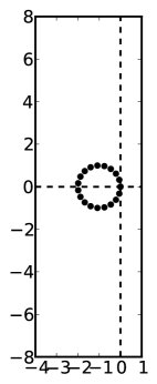
(a)

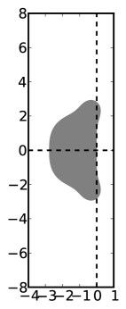
(b)

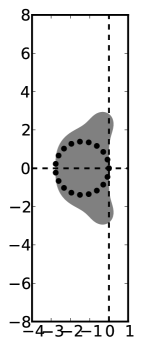
(c)

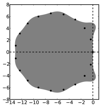
(d)

Figure 1: (a) spectrum of first-order upwind difference matrix using $N=20$ points in space; (b) stability region of the classical fourth-order Runge–Kutta method; (c) Scaled spectrum $h\lambda$ with $h=1.39$; (d) Scaled spectrum $h\lambda$ for optimal 10-stage method with $h=6.54$.

1.3 Design of optimal stability polynomials

We now consider the problem of choosing a stability polynomial so as to maximize the step size under which given stability constraints are satisfied. The objective function $f(x)$ is simply the step size $h$. The stability conditions yield nonlinear inequality constraints. Typically one also wishes to impose a minimal order of accuracy. The monomial basis representation (3) of $R(z)$ is then convenient because the first $p+1$ coefficients $\{a_{0},a_{1},\dots,a_{p}\}$ of the stability polynomial are simply taken to satisfy the order conditions (4). As a result, the space of decision variables has dimension $s+1-p$, and is comprised of the coefficients $\{a_{p+1},a_{p+2},\dots,a_{s}\}$, as well as the step size $h$. Then the problem can be written as

Problem 1 (stability optimization).

Given $\Lambda\subset\mathbb{C}$, order $p$, and number of stages $s$,

$$\operatorname*{maximize}_{a_{p+1},a_{p+2},\dots,a_{s},h} h$$

subject to $$|R(h\lambda)|-1\leq 0,\ \ \ \ \ \forall\lambda\in\Lambda.$$

We use $H_{\textup{opt}}$ to denote the solution of Problem 1 (the optimal step size) and $R_{\textup{opt}}$ to denote the optimal polynomial.

The set $\Lambda$ may be finite, corresponding to a finite-dimensional ODE system or PDE semi-discretization, or infinite (but bounded), corresponding to a PDE or perhaps its semi-discretization in the limit of infinitesimal mesh width. In the latter case, Problem 1 is a semi-infinite program (SIP). In Section 4 we approach this by using a finite discretization of $\Lambda$; for a discussion of this and other approaches to semi-infinite programming, see [14].

1.4 Previous work

The problem of finding optimal stability polynomials is of fundamental importance in the numerical solution of initial value problems, and its solution or approximation has been studied by many authors for several decades [23, 32, 42, 16, 17, 18, 45, 21, 20, 30, 22, 31, 43, 27, 26, 1, 3, 2, 44, 6, 37, 35, 5, 4, 25, 28, 38, 34]. Indeed, it is closely related to the problem of finding polynomials of least deviation, which goes back to the work of Chebyshev. A nice review of much of the early work on Runge–Kutta stability regions can be found in [43]. The most-studied cases are those where the eigenvalues lie on the negative real axis, on the imaginary axis, or in a disk of the form $|z+w|\leq w$. Many results and optimal polynomials, both exact and numerical, are available for these cases. Much less is available regarding the solution of Problem 1 for arbitrary spectra $\lambda_{i}$.

Two very recent works serve to illustrate both the progress that has been made in solving these problems with nonlinear programming, and the challenges that remain. In [38], optimal schemes are sought for integration of discontinuous Galerkin discretizations of wave equations, where the optimality criteria considered include both accuracy and stability measures. The approach used there is based on sequential quadratic programming (local optimization) with many initial guesses. The authors consider methods of at most fourth order and situations with $s-p\leq 4$ “because the cost of the optimization procedure becomes prohibitive for a higher number of free parameters.” In [28], optimally stable polynomials are found for certain spectra of interest for $2\leq p\leq 4$ and (in a remarkable feat!) $s$ as large as $14$. The new methods obtained achieve a 40-50% improvement in efficiency for discontinuous Galerkin integration of the 3D Maxwell equations. The optimization approach employed therein is again a direct search algorithm that does not guarantee a globally optimal solution but “typically converges … within a few minutes”. However, it was apparently unable to find solutions for $s>14$ or $p>4$. The method we present in the next section can rapidly find solutions for significantly larger values of $s,p$, and is provably globally convergent under certain assumptions (introduced in section 2).

2 An efficient algorithm for design of globally optimal stability polynomials

Evidently, finding the global solution of Problem 1 is in general quite challenging. Although the Karush-Kuhn-Tucker (KKT) conditions provide necessary conditions for optimality in the solution of nonlinear programming problems, the stability constraints in Problem 1 are nonconvex, hence suboptimal local minima may exist.

2.1 Reformulation in terms of the least deviation problem

The primary theoretical advance leading to the new results in this paper is a reformulation of Problem 1. Note that Problem 1 is (for $s>2$) nonconvex since $R(h\lambda)$ is a nonconvex function in $h$.

Instead of asking for the maximum stable step size we now ask, for a given step size $h$, how small the maximum modulus of $R(h\lambda)$ can be. This leads to a generalization of the classical least deviation problem.

Problem 2 ((Least Deviation)).

Given $\Lambda\subset\mathbb{C}$, $h\in\mathbb{R}^{+}$ and $p,s\in\mathbb{N}$

$$\operatorname*{minimize}_{a_{p+1},a_{p+2},\dots,a_{s}} \max_{\lambda\in\Lambda}\left(|R(h\lambda|-1\right).$$

We denote the solution of Problem 2 by $r_{p,s}(h,\Lambda)$, or simply $r(h,\Lambda)$. Note that $|R(z)|$ is convex with respect to $a_{j}$, since $R(z)$ is linear in the $a_{j}$. Therefore, Problem 2 is convex. Furthermore, Problem 1 can be formulated in terms of Problem 2.

Problem 3 (Reformulation of Problem 1).

Given $\Lambda\subset\mathbb{C}$, and $p,s\in\mathbb{N}$,

$$\operatorname*{maximize}_{a_{p+1},a_{p+2},\dots,a_{s}} h$$

subject to $$r_{p,s}(h,\Lambda)\leq 0.$$

2.2 Solution via bisection

Although Problem 3 is not known to be convex, it is an optimization in a single variable. It is natural then to apply a bisection approach, as outlined in Algorithm 1.

Algorithm 1 Simple bisection

$h_{\textup{min}}=0$

while $h_{\textup{max}}-h_{\textup{min}}>\epsilon$ do

     $h=(h_{\textup{max}}+h_{\textup{min}})/2$

     Solve Problem 2

     if $r_{p,s}(h,\Lambda)\leq 0$ then

         $h_{\textup{min}}=h$

     else

         $h_{\textup{max}}=h$

     end if

end while

return $H_{\epsilon}=h_{\textup{min}}$

As long as $h_{\textup{max}}$ is chosen large enough, it is clear that $r(h,\Lambda)=0$ for some $h\in[h_{\textup{min}},h_{\textup{max}}]$. Global convergence of the algorithm is assured only if the following condition holds:

$$r_{p,s}(h_{0},\Lambda)=0\implies r_{p,s}(h,\Lambda)\leq 0\text{ for all }0\leq h\leq h_{0}.$$ (8)

We now consider conditions under which condition (8) can be established. We have the following important case.

Theorem 1 (Global convergence when $p=1$).

Let $p=1$, $\Lambda\subset\mathbb{C}$ and $s\geq 1$. Take $h_{\textup{max}}$ large enough so that $r(h_{\textup{max}},\Lambda)>0$. Let $H_{\textup{opt}}$ denote the solution of Problem 1. Then the output of Algorithm 1 satisfies

$$\lim_{\epsilon\to 0}H_{\epsilon}=H_{\textup{opt}}.$$

Proof.

Since $r(0,\Lambda)=0<r(h_{\textup{max}},\Lambda)$ and $r(h,\Lambda)$ is continuous in $h$, it is sufficient to prove that condition (8) holds. We have $|R_{\textup{opt}}(H_{\textup{opt}}\lambda)|\leq 1$ for all $\lambda\in\Lambda$. We will show that there exists $R_{\mu}(z)=\sum_{j=0}^{s}a_{j}(\mu)z^{j}$ such that $a_{0}=a_{1}=1$ and

$$|R_{\mu}(\mu H_{\textup{opt}}\lambda)|\leq 1\ \ \ \forall\lambda\in\Lambda,\ \ 0\leq\mu\leq 1.$$

Let $\hat{a}_{j}$ be the coefficients of the optimal polynomial:

$$R_{\textup{opt}}(z)=1+z+\sum_{j=2}^{s}\hat{a}_{j}z^{j},$$

and set

$$a_{j}(\mu)=\mu^{1-j}\hat{a_{j}}.$$

Then

$$R_{\mu}(\mu H_{\textup{opt}}\lambda) =1+\mu H_{\textup{opt}}\lambda+\sum_{j=2}^{s}\mu^{1-j}\hat{a}_{j}\mu^{j}H_{\textup{opt}}^{j}\lambda^{j}=1+\mu\left(\sum_{j=1}^{s}\hat{a}_{j}H_{\textup{opt}}^{j}\lambda^{j}\right)$$

$$=1+\mu(R_{\textup{opt}}(H_{\textup{opt}}\lambda)-1),$$

where we have defined $\hat{a}_{1}=1$. Define $g_{\lambda}(\mu)=R_{\mu}(\mu H_{\textup{opt}}\lambda)$. Then $g_{\lambda}(\mu)$ is linear in $\mu$ and has the property that, for $\lambda\in\Lambda$, $|g_{\lambda}(0)|=1$ and $|g_{\lambda}(1)|\leq 1$ (by the definition of $H_{\textup{opt}},R_{\textup{opt}}$). Thus by convexity $|g(\mu)|\leq 1$ for $0\leq\mu\leq 1$. ∎

For $p>1$, condition (8) does not necessarily hold. For example, take $s=p=4$; then the stability polynomial (3) is uniquely defined as the degree-four Taylor approximation of the exponential, corresponding to the classical fourth-order Runge–Kutta method that we saw in the introduction. Its stability region is plotted in Figure 1(b). Taking, e.g., $\lambda=0.21+2.3i$, one finds $|R(\lambda)|<1$ but $|R(\lambda/2)|>1$. Although this example shows that Algorithm 1 might formally fail, it concerns only the trivial case $s=p$ in which there is only one possible choice of stability polynomial. We have searched without success for a situation with $s>p$ for which condition (8) is violated.

2.3 Convergence for starlike regions

In many important applications the relevant set $\Lambda$ is an infinite set; for instance, if we wish to design a method for some PDE semi-discretization that will be stable for any spatial discretization size. In this case, Problem 1 is a semi-infinite program (SIP) as it involves infinitely many constraints. Furthermore, $\Lambda$ is often a closed curve whose interior is starlike with respect to the origin; for example, upwind semi-discretizations of hyperbolic PDEs have this property. Recall that a region $S$ is starlike if $t\in S$ implies $\mu t\in S$ for all $0\leq\mu\leq 1$.

Lemma 1.

Let $\Lambda\in\mathbb{C}$ be a closed curve passing through the origin and enclosing a starlike region. Let $r(h,\Lambda)$ denote the solution of Problem 2. Then condition (8) holds.

Proof.

Let $\Lambda$ be as stated in the lemma. Suppose $r(h_{0},\Lambda)=0$ for some $h_{0}>0$; then there exists $R(z)$ such that $|R(h\lambda)|\leq 1$ for all $\lambda\in\Lambda$. According to the maximum principle, the stability region of $R(z)$ must contain the region enclosed by $\Lambda$. Choose $h$ such that $0\leq h\leq h_{0}$; then $h\Lambda$ lies in the region enclosed by $\Lambda$, so $|R(h\lambda)|\leq 1$ for $\lambda\in\Lambda$. ∎

The proof of Lemma 1 relies crucially on $\Lambda$ being an infinite set, but in practice we numerically solve Problem 2 with only finitely many constraints. To this end we introduce a sequence of discretizations $\Lambda_{n}$ with the following properties:

1. $\Lambda_{n}\subset\Lambda$

2. $n_{1}\leq n_{2}\implies\Lambda_{n_{1}}\subset\Lambda_{n_{2}}$

3. $\lim_{n\to\infty}\Lambda_{n}=\Lambda$

4. $\lim_{n\to\infty}\nu_{n}=0$ where $\nu_{n}$ denotes the maximum distance from a point in $\Lambda$ to the set $\Lambda_{n}$:

   $$\nu_{n}=\max_{\gamma\in\Lambda}\min_{\lambda\in\Lambda_{n}}|\gamma-\lambda|.$$

For instance, $\Lambda_{n}$ can be taken as an equispaced (in terms of arc-length, say) sampling of $n$ points.

By modifying Algorithm 1, we can approximate the solution of the semi-infinite programming problem for starlike regions to arbitrary accuracy. At each step we solve Problem 2 with $\Lambda_{n}$ replacing $\Lambda$. The key to the modified algorithm is to only increase $h_{\textup{min}}$ after obtaining a certificate of feasibility. This is done by using the Lipschitz constant of $R(z)$ over a domain including $h\Lambda$ (denoted by $L(R,h\Lambda)$) to ensure that $|R(h\Lambda)|\leq 1$. The modified algorithm is stated as Algorithm 2.

Algorithm 2 Bisection for SIP

$h_{\textup{min}}=0$

$h_{\textup{max}}=2s^{2}/\max|\lambda|$

$n=n_{0}$

while $h_{\textup{max}}-h_{\textup{min}}>\epsilon$ do

     $h=(h_{\textup{max}}+h_{\textup{min}})/2$ $\triangleright$ Bisect

     Solve Problem 2

     if $r(h,\Lambda_{n})<0$ and $\nu_{n}<-2r/L(R,h\Lambda)$ then $\triangleright$ Certifies that $r(h,\Lambda)<0$

         $h_{\textup{min}}=h$

     else if $r(h,\Lambda_{n})>0$ then $\triangleright$ Certifies that $r(h,\Lambda)>0$

         $h_{\textup{max}}=h$

     else$\triangleright$ $-\delta<r(h,\Lambda_{n})\leq 0$

         $n\leftarrow 2n$ $\triangleright$ Reduce the discretization spacing

     end if

end while

return $H_{\epsilon}=h_{\textup{min}}$

The following lemma, which characterizes the behavior of Algorithm 2, holds whether or not the interior of $\Lambda$ is starlike.

Lemma 2.

Let $h^{[k]}$ denote the value of $h$ after $k$ iterations of the loop in Algorithm 2. Then either

• Algorithm 2 terminates after a finite time with outputs satisfying $r(h_{\textup{min}},\Lambda)\leq 0$, $r(h_{\textup{max}},\Lambda)>0$; or

• there exists $j<\infty$ such that $r(h^{[j]},\Lambda)=0$ and $h^{[k]}=h^{[j]}$ for all $j\geq k$.

Proof.

First suppose that $r(h^{[j]},\Lambda)=0$ for some $j$. Then neither feasibility nor infeasibility can be certified for this value of $h$, so $h^{[k]}=h^{[j]}$ for all $j\geq k$.

On the other hand, suppose that $r(h^{[k]},\Lambda)\neq 0$ for all $k$. The algorithm will terminate as long as, for each $h^{[k]}$, either feasibility or infeasibility can be certified for large enough $n$. If $r(h^{[k]},\Lambda)>0$, then necessarily $r(h^{[k]},\Lambda_{n})>0$ for large enough $n$, so infeasibility will be certified. We will show that if $r(h^{[k]},\Lambda)<0$, then for large enough $n$ the condition

$$\nu_{n}<-2r/L(R,h\Lambda)$$ (9)

must be satisfied. Since $r(h,\Lambda_{n})\leq r(h,\Lambda)$ is bounded away from zero and $\lim_{n\to\infty}\nu_{n}=0$, (9) must be satisfied for large enough $n$ unless the Lipschitz constant $L(R,h\Lambda)$ is unbounded (with with respect to $n$) for some fixed $h$. Suppose by way of contradiction that this is the case, and let $R^{[1]},R^{[2]},\dots$ denote the corresponding sequence of optimal polynomials. Then the norm of the vector of coefficients $a_{j}^{[i]}$ appearing in $R^{[i]}$ must also grow without bound as $i\to\infty$. By Lemma 3, this implies that $|R^{[i]}(z)|$ is unbounded except for at most $s$ points $z\in\mathbb{C}$. But this contradicts the condition $|R^{[i]}(h\lambda)|\leq 1$ for $\lambda\in\Lambda_{n}$ when $n>s$. Thus, for large enough $n$ we must have $\nu_{n}<-2r/L(R,h\Lambda$). ∎

In practical application, $r(h,\Lambda)=0$ will not be detected, due to numerical errors; see Section 3.1. For this reason, in the next theorem we simply assume that Algorithm 2 terminates. We also require the following technical result, whose proof is deferred to the appendix.

Lemma 3.

Let $R^{[1]},R^{[2]},\dots$ be a sequence of polynomials of degree at most $s$ ($s\in\mathbb{N}$ fixed) and denote the coefficients of $R^{[i]}$ by $a_{j}^{[i]}\in\mathbb{C}$ ($i\in\mathbb{N}$, $0\leq j\leq s$):

$$R^{[i]}(z)=\sum_{j=0}^{s}a_{j}^{[i]}z^{j},\quad z\in\mathbb{C}.$$

Further, let $a^{[i]}:=(a_{0}^{[i]},a_{1}^{[i]},\dots,a_{s}^{[i]})^{T}$ and suppose that the sequence $\|a^{[i]}\|$ is unbounded in $\mathbb{R}$. Then the sequences $R^{[i]}(z)$ are unbounded for all but at most $s$ points $z\in\mathbb{C}$.

Proof.

Suppose to the contrary there are $s+1$ $\mathit{distinct}$ complex numbers, say, $z_{0},z_{1},\ldots,z_{s}$ such that the vectors $r_{i}:=(R^{[i]}(z_{0}),R^{[i]}(z_{1}),\ldots,R^{[i]}(z_{s}))^{T}$ ($i\in\mathbb{N}$) are bounded in $\mathbb{C}^{s+1}$. Let $V$ denote the $(s+1)\times(s+1)$ Vandermonde matrix whose $k^{\mathrm{th}}$ row ($0\leq k\leq s+1)$ is $(1,z_{k},z_{k}^{2},\ldots,z_{k}^{s})$. Then $V$ is invertible and we have $a^{[i]}=V^{-1}r_{i}$ ($i\in\mathbb{N}$), so if $\left|\!\left|\!\left|\cdot\right|\!\right|\!\right|$ denotes the induced matrix norm, then

$$\|a^{[i]}\|=\|V^{-1}r_{i}\|\leq\left|\!\left|\!\left|V^{-1}\right|\!\right|\!\right|\,\|r_{i}\|.$$

But, by assumption, the right hand side is bounded, whereas the left hand side is not. ∎

Theorem 2 (Global convergence for strictly starlike regions).

Let $\Lambda$ be a closed curve that encloses a region that is starlike with respect to the origin. Suppose that Algorithm 2 terminates for all small enough $\epsilon$, and let $H_{\epsilon}$ denote the value returned by Algorithm 2 for a given $\epsilon$. Let $H_{\textup{opt}}$ denote the solution of Problem 1. Then

$$\lim_{\epsilon\to 0}H_{\epsilon}=H_{\textup{opt}}.$$

Proof.

Due to the assumptions and Lemma 2, we have that $r(h_{\textup{min}},\Lambda)<0<r(h_{\textup{max}},\Lambda)$. Then Lemma 1 implies that $h_{\textup{min}}<H_{\textup{opt}}<h_{\textup{max}}$. Noting that also $h_{\textup{max}}-h_{\textup{min}}<\epsilon$, the result follows. ∎

Despite the lack of a general global convergence proof, Algorithm 1 works very well in practice even for general $\Lambda$ when $p>1$. In all cases we have tested and for which the true $H_{\textup{opt}}$ is known (see Section 4), Algorithm 1 appears to converge to the globally optimal solution. Furthermore, Algorithm 1 is very fast. For these reasons, we consider the (much slower) Algorithm 2 to be of primarily theoretical interest, and we base our practical implementation on Algorithm 1.

3 Numerical implementation

We have made a prototype implementation of Algorithm 1 in Matlab. The implementation relies heavily on the CVX package [12, 11], a Matlab-based modeling system for convex optimization, which in turn relies on the interior-point solvers SeDuMi [36] and SDPT3 [41]. The least deviation problem (Problem 2) can be succinctly stated in four lines of the CVX problem language, and for many cases is solved in under a second by either of the core solvers.

Our implementation re-attempts failed solves (see Section 3.2) with the alternate interfaced solver. In our test cases, we observed that the SDPT3 interior-point solver was slower, but more robust than SeDuMi. Consequently, our prototype implementation uses SDPT3 by default.

Using the resulting implementation, we were able to successfully solve problems to within $0.1\%$ accuracy or better with scaled eigenvalue magnitudes $|h\lambda|$ as large as 4000. As an example, comparing with results of [6] for spectra on the real axis with $p=3,s=27,$ our results are accurate to 6 significant digits.

3.1 Feasibility threshold

In practice, CVX often returns a small positive objective ($r\approx 10^{-7}$) for values of $h$ that are just feasible. Hence the bisection step is accepted if $r<\epsilon$ where $\epsilon\ll 1$. The results are generally insensitive (up to the first few digits) to the choice of $\epsilon$ over a large range of values; we have used $\epsilon=10^{-7}$ for all results in this work. The accuracy that can be achieved is eventually limited by the need to choose a suitable value $\epsilon$.

3.2 Conditioning and change of basis

Unfortunately, for large values of $h\lambda$, the numerical solution of Problem 2 becomes difficult due to ill-conditioning of the constraint matrix. Observe from (3) that the constrained quantities $R(h\lambda)$ are related to the decision variables $a_{j}$ through multiplication by a Vandermonde matrix. Vandermonde matrices are known to be ill-conditioned for most choices of abscissas. For very large $h\lambda$, the resulting CVX problem cannot be reliably solved by either of the core solvers.

A first approach to reducing the condition number of the constraint matrix is to rescale the monomial basis. We have found that a more robust approach for many types of spectra can be obtained by choosing a basis that is approximately orthogonal over the given spectrum $\{\Lambda\}$. Thus we seek a solution of the form

$$R(z) =\sum_{j=0}^{s}a_{j}Q_{j}(z) \mbox{where }\quad\quad\quad Q_{j}(z) =\sum_{k=0}^{j}b_{jk}z^{k}.$$ (10)

Here $Q_{j}(z)$ is a degree-$j$ polynomial chosen to give a well-conditioned constraint matrix. The drawback of not using the monomial basis is that the dimension of the problem is $s+1$ (rather than $s+1-p$) and we must now impose the order conditions explicitly:

$$\sum_{j=0}^{s}a_{j}b_{jk}=\frac{1}{k!}\quad\quad\mbox{ for }\ \ k=0,1,\dots,p.$$ (11)

Consequently, using a non-monomial basis increases the number of design variables in the problem and introduces an equality constraint matrix $B\in\mathbb{R}^{p\times s}$ that is relatively small (when $p\ll s$), but usually very poorly conditioned. However, it can dramatically improve the conditioning of the inequality constraints.

The choice of the basis $Q_{j}(z)$ is a challenging problem in general. In the special case of a negative real spectrum, an obvious choice is the Chebyshev polynomials (of the first kind) $T_{j}$, shifted and scaled to the domain $[hx,0]$ where $x=\min_{\lambda\in\Lambda}\operatorname{Re}(\lambda)$, via an affine map:

$$Q_{j}(z) =T_{j}\left(1+\frac{2z}{hx}\right).$$ (12)

The motivation for using this basis is that $|Q_{j}(h\lambda)|\leq 1$ for all $\lambda\in[hx,0]$. This basis is also suggested by the fact that $Q_{j}(z)$ is the optimal stability polynomial in terms of negative real axis inclusion for $p=1,s=j$. In Section 4, we will see that this choice of basis works well for more general spectra when the largest magnitude eigenvalues lie near the negative real axis.

As an example, we consider a spectrum of 3200 equally spaced values $\lambda$ in the interval $[-1,0]$. The exact solution is known to be $h=2s^{2}$. Figure 2 shows the relative error as well as the inequality constraint matrix condition number obtained by using the monomial (3) and Chebyshev (12) bases. Typically, the solver is accurate until the condition number reaches about $10^{16}$. This supports the hypothesis that it is the conditioning of the inequality constraint matrix that leads to failure of the solver. The Chebyshev basis keeps the condition number small and yields accurate answers even for very large values of $h$.

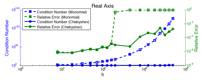
Figure 2: Condition number of principal constraint matrix and relative solution accuracy versus optimal step size. The points along a given curve correspond to different choices of $s$.

3.3 Choice of initial upper bound

The bisection algorithm requires as input an initial $h_{\textup{max}}$ such that $r(h_{\textup{max}},\Lambda)>0$. Theoretical values can be obtained using the classical upper bound of $2s^{2}/x$ if $\Lambda$ encloses a negative real interval $[x,0]$, or using the upper bound given in [33] if $\Lambda$ encloses an ellipse in the left half-plane. Alternatively, one could start with a guess and successively double it until $r(h_{\textup{max}},\Lambda)>0$ is satisfied. Since evaluation of $r(h,\Lambda)$ is typically quite fast, finding a tight initial $h_{\textup{max}}$ is not an essential concern.

4 Examples

We now demonstrate the effectiveness of our algorithm by applying it to determine optimally stable polynomials (i.e., solve Problem 1) for various types of spectra. As stated above, we use Algorithm 1 for its simplicity, speed, and effectiveness. When $\Lambda$ corresponds to an infinite set, we approximate it by a fine discretization.

4.1 Verification

In this section, we apply our algorithm to some well-studied cases with known exact or approximate results in order to verify its accuracy and correctness. In addition to the real axis, imaginary axis, and disk cases below, we have successfully recovered the results of [28]. Our algorithm succeeds in finding the globally optimal solution in every case for which it is known, except in some cases of extremely large step sizes for which the underlying solvers (SDPT3 and SeDuMi) eventually fail.

4.1.1 Negative real axis inclusion

Here we consider the largest $h$ such that $[-h,0]\in S$ by taking $\Lambda=[-1,0]$. This is the most heavily studied case in the literature, as it applies to the semi-discretization of parabolic PDEs and a large increase of $H_{\textup{opt}}$ is possible when $s$ is increased (see, e.g., [32, 43, 27, 6, 34]). For first-order accurate methods ($p=1$), the optimal polynomials are just shifted Chebyshev polynomials, and the optimal timestep is $H_{\textup{opt}}=2s^{2}$. Many special analytical and numerical techniques have been developed for this case; the most powerful seems to be that of Bogatyrev [6].

We apply our algorithm to a discretization of $\Lambda$ (using 6400 evenly-spaced points) and using the shifted and scaled Chebyshev basis (12). Results for up to $s=40$ are shown in Table 1 (note that we list $H_{\textup{opt}}/s^{2}$ for easy comparison, since $H_{\textup{opt}}$ is approximately proportional to $s^{2}$ in this case). We include results for $p=10$ to demonstrate the algorithm’s ability to handle high-order methods. For $p=1$ and $2$, the values computed here match those available in the literature [42]. Most of the values for $p=3,4$ and $10$ are new results. Figure 3 shows some examples of stability regions for optimal methods. As observed in the literature, it seems that $H_{\textup{opt}}/s^{2}$ tends to a constant (that depends only on $p$) as $s$ increases. For large values of $s$, some results in the table have an error of about $10^{-3}$ due to inaccuracies in the numerical results provided by the interior point solvers.

	$H_{\textup{opt}}/s^{2}$
Stages	$p=1$	$p=2$	$p=3$	$p=4$	$p=10$
1	2.000
2	2.000	0.500
3	2.000	0.696	0.279
4	2.000	0.753	0.377	0.174
5	2.000	0.778	0.421	0.242
6	2.000	0.792	0.446	0.277
7	2.000	0.800	0.460	0.298
8	2.000	0.805	0.470	0.311
9	2.000	0.809	0.476	0.321
10	2.000	0.811	0.481	0.327	0.051
15	2.000	0.817	0.492	0.343	0.089
20	2.000	0.819	0.496	0.349	0.120
25	2.000	0.820	0.498	0.352	0.125
30	2.001	0.821	0.499	0.353	0.129
35	2.000	0.821	0.499	0.354	0.132
40	2.000	0.821	0.500	0.355	0.132

Table 1: Scaled size of real axis interval inclusion for optimized methods.

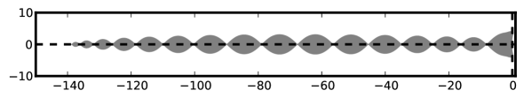
(a) $p=4,s=20$

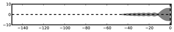
(b) $p=10,s=20$

Figure 3: Stability regions of some optimal methods for real axis inclusion.

4.1.2 Imaginary axis inclusion

Next we consider the largest $h$ such that $[-ih,ih]\in S$ by taking $\Lambda=xi,x\in[-1,1]$. Optimal polynomials for imaginary axis inclusion have also been studied by many authors, and a number of exact results are known or conjectured [42, 45, 20, 21, 22, 43]. We again approximate the problem, taking $N=3200$ evenly-spaced values in the interval $[0,i]$ (note that stability regions are necessarily symmetric about the real axis since $R(z)$ has real coefficients). We use a “rotated” Chebyshev basis defined by

$$Q_{j}(z)=i^{j}T_{j}\left(\frac{iz}{hx}\right),$$

where $x=\max_{i}(|\operatorname{Im}(\lambda_{i})|)$. Like the Chebyshev basis for the negative real axis, this basis dramatically improves the robustness of the algorithm for imaginary spectra. Table 2 shows the optimal effective step sizes. In agreement with [42, 21], we find $H=s-1$ for $p=1$ (all $s$) and for $p=2$ ($s$ odd). We also find $H=s-1$ for $p=1$ and $s$ even, which was conjectured in [45] and confirmed in [43]. We find $H_{\textup{opt}}=\sqrt{s(s-2)}$ for $p=2$ and $s$ even, strongly suggesting that the polynomials given in [20] are optimal for these cases; on the other hand, our results show that those polynomials, while third order accurate, are not optimal for $p=3$ and $s$ odd. Figure 4 shows some examples of stability regions for optimal methods.

	$H_{\textup{opt}}/s$
Stages	$p=1$	$p=2$	$p=3$	$p=4$
2	0.500
3	0.667	0.667	0.577
4	0.750	0.708	0.708	0.707
5	0.800	0.800	0.783	0.693
6	0.833	0.817	0.815	0.816
7	0.857	0.857	0.849	0.813
8	0.875	0.866	0.866	0.866
9	0.889	0.889	0.884	0.864
10	0.900	0.895	0.895	0.894
15	0.933	0.933	0.932	0.925
20	0.950	0.949	0.949	0.949
25	0.960	0.960	0.959	0.957
30	0.967	0.966	0.966	0.966
35	0.971	0.971	0.971	0.970
40	0.975	0.975	0.975	0.975
45	0.978	0.978	0.978	0.977
50	0.980	0.980	0.980	0.980

Table 2: Scaled size of imaginary axis inclusion for optimized methods.

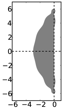
(a) $p=1,s=7$

(b) $p=4,s=7$

Figure 4: Stability regions of some optimal methods for imaginary axis inclusion.

4.1.3 Disk inclusion

In the literature, attention has been paid to stability regions that include the disk

$$D(h) =\{z:|1+z/h|\leq 1\},$$ (13)

for the largest possible $h$. As far as we know, the optimal result for $p=1$ ($H_{\textup{opt}}=s$) was first proved in [16]. The optimal result for $p=2$ ($H_{\textup{opt}}=s-1$) was first proved in [45]. Both results have been unwittingly rediscovered by later authors. For $p>2$, no exact results are available.

We use the basis

$$Q_{j}(z)=\left(1+\frac{z}{h}\right)^{j}.$$

Note that $Q_{j}(z)$ is the optimal polynomial for the case $s=j$, $p=1$. This basis can also be motivated by recalling that Vandermonde matrices are perfectly conditioned when the points involved are equally spaced on the unit circle. Our basis can be obtained by taking the monomial basis and applying an affine transformation that shifts the unit circle to the disk (13). This basis greatly improves the robustness of the algorithm for this particular spectrum. We show results for $p\leq 4$ in Figure 5. For $p=3$ and $s=5,6$, our results give a small improvement over those of [19]. Some examples of optimal stability regions are plotted in Figure 6.

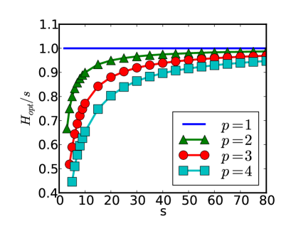
Figure 5: Relative size of largest disk that can be included in the stability region (scaled by the number of stages).

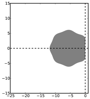
(a) $p=3,s=8$

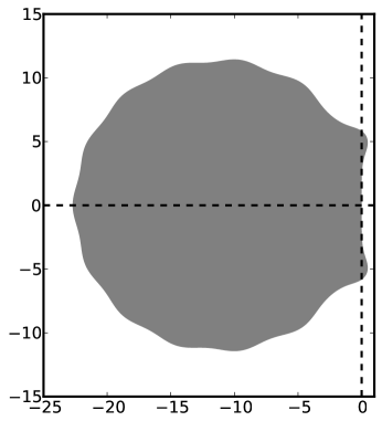
(b) $p=4,s=15$

Figure 6: Stability regions of some optimal methods for disk inclusion.

4.2 Spectrum with a gap

We now demonstrate the effectiveness of our method for more general spectra. First we consider the case of a dissipative problem with two time scales, one much faster than the other. This type of problem was the motivation for the development of projective integrators in [9]. Following the ideas outlined there we consider

$$\Lambda =\{z:|z|=1,\mathbb{R}(z)\leq 0\}\cup\{z:|z-\alpha|=1\}.$$ (14)

We take $\alpha=20$ and use the shifted and scaled Chebyshev basis (12). Results are shown in Figure 7. A dramatic increase in efficiency is achieved by adding a few extra stages.

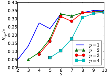
(a) Optimal effective step size

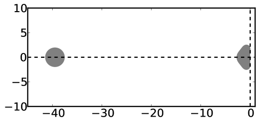
(b) Optimal stability region for $p=1,s=6,\alpha=20$ (stable step size $\approx 1.975$)

Figure 7: Optimal methods for spectrum with a gap (14) with $\alpha=20$.

4.3 Legendre pseudospectral discretization

Next we consider a system obtained from semidiscretization of the advection equation on the interval $[-1,1]$ with homogeneous Dirichlet boundary condition:

$$u_{t}=u_{x}\ \ \ \ \ \ \ \ u(t,x=1)=0.$$

The semi-discretization is based on pseudospectral collocation at points given by the zeros of the Legendre polynomials; we take $N=50$ points. The semi-discrete system takes the form (1), where $L$ is the Legendre differentiation matrix, whose eigenvalues are shown in Figure 8(a). We compute an optimally stable polynomial based on the spectrum of the matrix, taking $s=7$ and $p=1$. The stability region of the resulting method is plotted in Figure 8(c). Using an appropriate step size, all the scaled eigenvalues of $L$ lie in the stability region. However, this method is unstable in practice for any positive step size; Figure 8(e) shows an example of a computed solution after three steps, where the initial condition is a Gaussian. The resulting instability is non-modal, meaning that it does not correspond to any of the eigenvectors of $L$ (compare [40, Figure 31.2]).

This discretization is now well-known as an example of non-normality [40, Chapters 30-32]. Due to the non-normality, it is necessary to consider pseudospectra in order to design an appropriate integration scheme. The $\epsilon$-pseudospectrum (see [40]) is the set

$$\{z\in\mathbb{C}:\|(z-D)^{-1}\|>1/\epsilon\}.$$

The $\epsilon$-pseudospectrum (for $\epsilon=2$) is shown with the eigenvalues in Figure 8(b). The instability observed above occurs because the stability region does not contain an interval on the imaginary axis about the origin, whereas the pseudospectrum includes such an interval.

We now compute an optimally stable integrator based on the 2-pseudospectrum. This pseudospectrum is computed using an approach proposed in [39, Section 20], with sampling on a fine grid. In order to reduce the number of constraints and speed up the solution, we compute the convex hull of the resulting set and apply our algorithm. The resulting stability region is shown in Figure 8(d). It is remarkably well adapted; notice the two isolated roots that ensure stability of the modes corresponding to the extremal imaginary eigenvalues. We have verified that this method produces a stable solution, in agreement with theory (see Chapter 32 of [40]); Figure 8(f) shows an example of a solution computed with this method. The initial Gaussian pulse advects to the left.

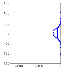
(a) Eigenvalues.

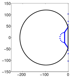
(b) Eigenvalues and pseudospectrum (the boundary of the 2-pseudospectrum is plotted).

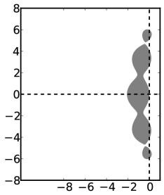
(c) Optimized stability region based on eigenvalues.

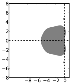
(d) Optimized stability region based on pseudospectrum.

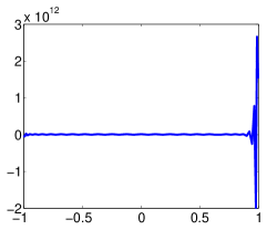
(e) Solution computed with method based on spectrum.

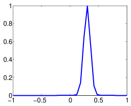
(f) Solution computed with method based on pseudospectrum.

Figure 8: Results for the Legendre differentiation matrix with $N=50$.

4.4 Thin rectangles

A major application of explicit Runge–Kutta methods with many stages is the solution of moderately stiff advection-reaction-diffusion problems [15, 44]. For such problems, the stability region must include not only a large interval on the negative real axis, but also some region around it, due to convective terms. If centered differences are used for the advective terms, it is natural to require that a small interval on the imaginary axis be included. Hence, one may be interested in methods that contain a rectangular region

$$\Lambda_{\kappa}=\{\lambda\in\mathbb{C}:-\beta\leq\operatorname{Im}(\lambda)\leq\beta,\ \ -\kappa\leq\real(\lambda)\leq 0\}.$$ (15)

for given $\kappa,\beta$. No methods optimized for such regions appear in the literature, and the available approaches for devising methods with extended real axis stability (including those of [37]) cannot be applied to such regions. Because of this, previously existing methods are applicable only if upwind differencing is applied to convective terms [44, 37].

For this example, rather than parameterizing by the step size $h$, we assume that a desired step size $h$ and imaginary axis limit $\beta$ are given based on the convective terms, which generally require small step sizes for accurate resolution. We seek to find (for given $s,p$) the polynomial (3) that includes $\Lambda_{\kappa}$ for $\kappa$ as large as possible. This could correspond to selection of an optimal integrator based on the ratio of convective and diffusive scales (roughly speaking, the Reynolds number). Since the desired stability region lies relatively near the negative real axis, we use the shifted and scaled Chebyshev basis (12).

Stability regions of some optimal methods are shown in Figure 9. The outline of the included rectangle is superimposed in black. The stability region for $\beta=10,s=20$, shown in Figure 9 is especially interesting as it is very nearly rectangular. A closeup view of the upper boundary is shown in Figure 10.

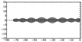
(a) $\beta=1$, $p=1,s=10$

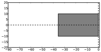
(b) $\beta=10$, $p=1,s=20$

Figure 9: Stability regions of some optimal methods for thin rectangle inclusion.

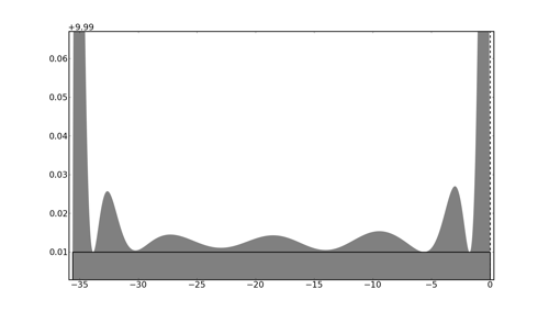
Figure 10: Closeup view of upper boundary of the rectangular stability region plotted in Figure 9.

5 Discussion

The approach described here can speed up the integration of IVPs for which

• explicit Runge–Kutta methods are appropriate;

• the spectrum of the problem is known or can be approximated; and

• stability is the limiting factor in choosing the step size.

Although we have considered only linear initial value problems, we expect our approach to be useful in designing integrators for nonlinear problems via the usual approach of considering the spectrum of the Jacobian. A first successful application of our approach to nonlinear PDEs appears in [29].

The amount of speedup depends strongly on the spectrum of the problem, and can range from a few percent to several times or more. Based on past work and on results presented in Section 4, we expect that the most substantial gains in efficiency will be realized for systems whose spectra have large negative real parts, such as for semi-discretization of PDEs with significant diffusive or moderately stiff reaction components. As demonstrated in Section 4, worthwhile improvements may also be attained for general systems, and especially for systems whose spectrum contains gaps.

The work presented here suggests several extensions and areas for further study. For very high polynomial degree, the convex subproblems required by our algorithm exhibit poor numerical conditioning. We have proposed a first improvement by change of basis, but further improvements in this regard could increase the robustness and accuracy of the algorithm. It seems likely that our algorithm exhibits global convergence in general circumstances beyond those for which we have proven convergence. The question of why bisection seems to always lead to globally optimal solutions merits further investigation. While we have focused primarily on design of the stability properties of a scheme, the same approach can be used to optimize accuracy efficiency, which is a focus of future work. Our algorithm can also be applied in other ways; for instance, it could be used to impose a specific desired amount of dissipation for use in multigrid or as a kind of filtering.

We remark that the problem of determining optimal polynomials subject to convex constraints is very general. Convex optimization techniques have already been exploited to solve similar problems in filter design [8], and will likely find further applications in numerical analysis.

Acknowledgments. We thank Lajos Loczi for providing a simplification of the proof of Lemma 3. We are grateful to R.J. LeVeque and L.N. Trefethen for helpful comments on a draft of this work.

References

- [1] A. Abdulle, On roots and error constants of optimal stability polynomials, BIT Numerical Mathematics, 40 (2000), pp. 177–182.
- [2] , Fourth order Chebyshev methods with recurrence relation, SIAM Journal on Scientific Computing, 23 (2002), pp. 2041–2054.
- [3] A. Abdulle and A. Medovikov, Second order Chebyshev methods based on orthogonal polynomials, Numerische Mathematik, 90 (2001), pp. 1–18.
- [4] V. Allampalli, R. Hixon, M. Nallasamy, and S. D. Sawyer, High-accuracy large-step explicit Runge-Kutta (HALE-RK) schemes for computational aeroacoustics, Journal of Computational Physics, 228 (2009), pp. 3837–3850.
- [5] M. Bernardini and S. Pirozzoli, A general strategy for the optimization of Runge–-Kutta schemes for wave propagation phenomena, Journal of Computational Physics, 228 (2009), pp. 4182–4199.
- [6] A. B. Bogatyrev, Effective solution of the problem of the optimal stability polynomial, Sbornik: Mathematics, 196 (2005), pp. 959–981.
- [7] J. Butcher, Numerical Methods for Ordinary Differential Equations, Wiley, second ed., 2008.
- [8] T. Davidson, Enriching the Art of FIR Filter Design via Convex Optimization, IEEE Signal Processing Magazine, 27 (2010), pp. 89–101.
- [9] C. W. Gear and I. G. Kevrekidis, Projective Methods for Stiff Differential Equations: Problems with Gaps in Their Eigenvalue Spectrum, SIAM Journal on Scientific Computing, 24 (2003), p. 1091.
- [10] S. Gottlieb, D. I. Ketcheson, and C.-W. Shu, Strong stability preserving Runge–Kutta and multistep time discretizations, World Scientific Publishing Company, 2011.
- [11] M. Grant and S. Boyd, Graph implementations for nonsmooth convex programs, in Recent Advances in Learning and Control, V. Blondel, S. Boyd, and H. Kimura, eds., Lecture Notes in Control and Information Sciences, Springer-Verlag Limited, 2008, pp. 95–110.
- [12] , CVX: MATLAB software for disciplined convex programming. http://cvxr.com/cvx, Apr. 2011.
- [13] E. Hairer, , and G. Wanner, Solving ordinary differential equations II: Stiff and differential-algebraic problems, Springer, second ed., 1996.
- [14] R. Hettich, Semi-Infinite Programming: Theory, Methods, and Applications, SIAM review, 35 (1993), pp. 380–429.
- [15] W. Hundsdorfer and J. G. Verwer, Numerical solution of time-dependent advection-diffusion-reaction equations, vol. 33, Springer, 2003.
- [16] R. Jeltsch and O. Nevanlinna, Largest disk of stability of explicit Runge–Kutta methods, BIT Numerical Mathematics, 18 (1978), pp. 500–502.
- [17] , Stability of explicit time discretizations for solving initial value problems, Numerische Mathematik, 37 (1981), pp. 61–91.
- [18] , Stability and accuracy of time discretizations for initial value problems, Numerische Mathematik, 40 (1982), pp. 245–296.
- [19] R. Jeltsch and M. Torrilhon, Flexible stability domains for explicit Runge–Kutta methods, Some topics in industrial and applied mathematics, (2007), p. 152.
- [20] I. P. Kinnmark and W. G. Gray, One step integration methods of third-fourth order accuracy with large hyperbolic stability limits, Mathematics and Computers in Simulation, 26 (1984), pp. 181–188.
- [21] , One step integration methods with maximum stability regions, Mathematics and Computers in Simulation, 26 (1984), pp. 87–92.
- [22] I. P. E. Kinnmark and W. G. Gray, Fourth-order accurate one-step integration methods with large imaginary stability limits, Numerical Methods for Partial Differential Equations, 2 (1986), pp. 63–70.
- [23] J. Lawson, An order five Runge–Kutta process with extended region of stability, SIAM Journal on Numerical Analysis, (1966).
- [24] R. J. LeVeque, Finite Difference Methods for Ordinary and Partial Differential Equations, SIAM, Philadelphia, 2007.
- [25] J. Martin-Vaquero and B. Janssen, Second-order stabilized explicit Runge–Kutta methods for stiff problems, Computer Physics Communications, 180 (2009), pp. 1802–1810.
- [26] J. L. Mead and R. A. Renaut, Optimal Runge–Kutta methods for first order pseudospectral operators, Journal of Computational Physics, 152 (1999), pp. 404–419.
- [27] A. A. Medovikov, High order explicit methods for parabolic equations, BIT Numerical Mathematics, 38 (1998), pp. 372–390.
- [28] J. Niegemann, R. Diehl, and K. Busch, Efficient low-storage Runge-Kutta schemes with optimized stability regions, Journal of Computational Physics, 231 (2011), pp. 372–364.
- [29] M. Parsani et al., Optimal explicit Runge–Kutta schemes for the spectral difference method applied to Euler and linearized Euler equations. In Preparation.
- [30] J. Pike and P. Roe, Accelerated convergence of Jameson’s finite-volume Euler scheme using van der Houwen integrators, Computers & Fluids, 13 (1985), pp. 223–236.
- [31] R. Renaut, Two-step Runge-Kutta methods and hyperbolic partial differential equations, Mathematics of Computation, 55 (1990), pp. 563–579.
- [32] W. Riha, Optimal stability polynomials, Computing, 9 (1972), pp. 37–43.
- [33] J. M. Sanz-Serna and M. N. Spijker, Regions of stability, equivalence theorems and the Courant-Friedrichs-Lewy condition, Numerische Mathematik, 49 (1986), pp. 319–329.
- [34] L. M. Skvortsov, Explicit stabilized Runge–Kutta methods, Computational Mathematics and Mathematical Physics, 51 (2011), pp. 1153–1166.
- [35] B. Sommeijer and J. G. Verwer, On stabilized integration for time-dependent PDEs, Journal of Computational Physics, 224 (2007), pp. 3–16.
- [36] J. Sturm, Using sedumi 1.02, a matlab toolbox for optimization over symmetric cones, Optimization methods and software, 11 (1999), pp. 625–653.
- [37] M. Torrilhon and R. Jeltsch, Essentially optimal explicit Runge-Kutta methods with application to hyperbolic–parabolic equations, Numerische Mathematik, 106 (2007), pp. 303–334.
- [38] T. Toulorge and W. Desmet, Optimal Runge–Kutta Schemes for Discontinuous Galerkin Space Discretizations Applied to Wave Propagation Problems, Journal of Computational Physics, (2011).
- [39] L. Trefethen, Computation of pseudospectra, Acta numerica, 8 (1999), pp. 247–295.
- [40] L. Trefethen and M. Embree, Spectra and Pseudospectra: The Behavior of Nonnormal Matrices and Operators, Princeton University Press, Princeton, 2005.
- [41] R. Tütüncü, K. Toh, and M. Todd, Solving semidefinite-quadratic-linear programs using sdpt3, Mathematical programming, 95 (2003), pp. 189–217.
- [42] P. van der Houwen, Explicit Runge–Kutta Formulas with Increased Stability Boundaries, Numerische Mathematik, 20 (1972), pp. 149–164.
- [43] P. J. van der Houwen, The development of Runge–Kutta methods for partial differential equations, Applied Numerical Mathematics, 20 (1996), pp. 261––272.
- [44] J. G. Verwer, B. Sommeijer, and W. Hundsdorfer, RKC time-stepping for advection-diffusion-reaction problems, Journal of Computational Physics, 201 (2004), pp. 61–79.
- [45] R. Vichnevetsky, New stability theorems concerning one-step numerical methods for ordinary differential equations, Mathematics and Computers in Simulation, 25 (1983), pp. 199–205.