Massive photons and Lorentz violation

Abstract

All quadratic translation- and gauge-invariant photon operators for Lorentz breakdown are included into the Stueckelberg Lagrangian for massive photons in a generalized $R_{\xi}$ gauge. The corresponding dispersion relation and tree-level propagator are determined exactly, and some leading-order results are derived. The question of how to include such Lorentz-violating effects into a perturbative quantum-field expansion is addressed. Applications of these results within Lorentz-breaking quantum field theories include the regularization of infrared divergences as well as the free propagation of massive vector bosons.

I introduction

Recent years have witnessed a growing interest in precision tests of Lorentz and CPT invariance. This interest can be partly attributed to the availability of new observational data and the development of ultra-sensitive experimental techniques ExpRev . Moreover, minute departures from Lorentz and CPT symmetry can be accommodated in various theoretical ideas beyond established physics motivation providing a phenomenological opportunity to search for novel effects possibly arising at the Planck scale.

At presently attainable energies, Lorentz- and CPT-violating effects are expected to be governed by effective field theory EFT . The general framework based on this premise is known as the Standard-Model Extension (SME) SMEpapers ; caus ; PhotonSME . This framework contains the usual Standard Model of particle physics and general relativity as limiting cases and therefore permits the identification and analysis of essentially all currently feasible Lorentz and CPT tests. To date, the SME has been employed for phenomenological studies involving cosmic radiation UHECR , meson factories mesons and other particle colliders collider , resonance cavities cavities , neutrinos neutrinos , precision spectroscopy spectroscopy , and gravity GravExp .

The SME has also served as the basis for various theoretical investigations of Lorentz and CPT symmetry. These investigations have have shed light on the SME’s mathematical structure math , spontaneous Lorentz breakdown and Nambu–Goldstone modes SSB , classical limits of Lorentz- and CPT-violating physics classical , quantum corrections and renormalizability loops ; AACGS , features of non-renormalizable contributions nonren , etc. At the same time, these analyses have solidified various aspects of the SME’s theoretical foundation.

One topic that has remained comparatively unexplored concerns Lorentz and CPT violations in massive vector particles in the SME: published work EWpaper has been focused on phenomenological analyses confined to the CPT-even $Z^{0}$ and $W^{\pm}$ sectors of the minimal SME. However, even for this small region in the full SME’s parameter space basic theoretical results, such as expressions for the dispersion relation and propagator, are currently still lacking. The present investigation reports on progress towards filling this gap.

Massive vector particles with Lorentz and CPT breaking are not only of interest for phenomenological studies of the heavy gauge bosons $Z^{0}$ and $W^{\pm}$. They have previously served a valuable tool for investigations of the mass-dimension three Lorentz- and CPT-violating Maxwell–Chern–Simons term AACGS . More importantly, massive vector fields play a key role for theoretical studies involving the photon because they provide a popular method for regularizing infrared divergences in perturbative quantum-field calculations. In fact, this latter application represents the primary focus of this study. But we anticipate that our results for the expression of the dispersion relation and the propagator are equally valid for the quadratic part of the full SME’s $Z^{0}$ and $W^{\pm}$ sectors.

The outline of the present work is as follows. Section II provides the basic ideas behind the construction of the model we are studying. A few remarks on the structure of the resulting modified Maxwell–Stueckelberg equations are contained in Sec. III. Section IV determines the exact dispersion relation and propagator for our model. Section V discusses some leading-order results that are expected to be useful for practical calculations, and Sec. VI gives a brief summary of our results. Some supplementary material is collected in various appendices.

II Model Basics

Our primary goal is to introduce a photon mass for regularizing infrared divergences in perturbative quantum-field calculations in a general $R_{\xi}$ gauge. This requires a smooth behavior of the internal-symmetry structure in the massless limit. Thus, the usual Proca term by itself is insufficient, and the mass needs to be introduced via, e.g., the Stueckelberg method Stueckelberg . The original version of this method is appropriate for U(1) gauge theories. The method needs modifications for photons embedded in the U(1)$\times$SU(2) gauge structure of the Standard Model StueckelbergSM , and it generally fails for non-Abelian vector fields. The Lorentz-violating generalization of the Stueckelberg method, which is discussed in this section and the subsequent one, therefore applies solely to the SME’s QED limit. We do, however, expect the remaining part of our study, contained in Secs. IV and V, to be applicable to more general massive vector fields.

Our starting point is the usual free-photon Lagrangian minimally coupled to an external conserved current $j^{\mu}$. The generalization of this Lagrangian to include arbitrary local, coordinate-independent, translation- and gauge-invariant physics with Lorentz- and CPT-symmetry breakdown can be cast into the following form PhotonSME :

$${}{\cal L}_{\gamma}\! = \!-\tfrac{1}{4}F^{2}-A\cdot j$$ (1)

$${}-\tfrac{1}{4}F_{\kappa\lambda}(\hat{k}_{F})^{\kappa\lambda\mu\nu}F_{\mu\nu}+\tfrac{1}{2}\epsilon^{\kappa\lambda\mu\nu}A_{\lambda}(\hat{k}_{AF})_{\kappa}F_{\mu\nu}\,.$$

Here, the field strengths and potentials are real-valued and obey the conventional relation $F_{\mu\nu}=\partial_{\mu}A_{\nu}-\partial_{\nu}A_{\mu}$, and $\epsilon^{\kappa\lambda\mu\nu}$ denotes the totally antisymmetric symbol with $\epsilon^{0123}=+1$. Lorentz and CPT breakdown is controlled by the quantities $\hat{k}_{F}$ and $\hat{k}_{AF}$, which are given explicitly by the following expressions PhotonSME

$${}(\hat{k}_{F})^{\kappa\lambda\mu\nu}\! = \!\sum_{n=2}^{\infty}(k_{F}^{(2n)})^{\kappa\lambda\mu\nu\alpha_{1}\ldots\alpha_{2n-4}}\partial_{\alpha_{1}}\ldots\partial_{\alpha_{2n-4}}$$

$$(\hat{k}_{AF})_{\kappa}\! = \!\sum_{n=1}^{\infty}(k_{AF}^{(2n+1)})_{\kappa}{}^{\alpha_{1}\ldots\alpha_{2n-2}}\partial_{\alpha_{1}}\ldots\partial_{\alpha_{2n-2}}\,.$$ (2)

Each $k_{F}^{(d)}$ coefficient as well as each $k_{AF}^{(d)}$ coefficient is taken as nondynamical, spacetime constant, and totally symmetric in its $\alpha$ indices. The superscript $(d)$ labels the mass dimension of the corresponding photon operator, so that the unit of the actual coefficient is $[\textrm{GeV}]^{\,4-d}$.

The next step is to add a mass-type term $\delta{\cal L}_{m}$ for the photon to the above Lagrangian (1). In the conventional case, such a contribution is restricted by Lorentz symmetry. In the present situation, this restriction is absent, and more freedom in the choice of $\delta{\cal L}_{m}$ exists. This additional freedom partly depends on the type of physics to be described. For instance, one may wish to model general Lorentz violation for hypothetical massive photons. Alternatively, the aim may be to regularize infrared divergences that often arise in quantum-field calculations involving massless photons governed by Lagrangian (1). In these two examples, the former may allow more additional freedom for $\delta{\cal L}_{m}$ than the latter: consider a situation in which the coefficients in Lagrangian (1) are such that a subgroup of the Lorentz group remains intact. A regulator breaking this residual symmetry may be problematic, so that violations of the remaining invariant subgroup may have to be excluded from $\delta{\cal L}_{m}$.

In the present work, the primary purpose for the introduction of a photon-mass term is to regularize potential infrared divergences in quantum-field contexts. In principle, the structure of $\delta{\cal L}_{m}$ can then be chosen as simple as possible. For example, the conventional Lorentz-symmetric Stueckelberg expression would likely suffice.

However, we introduce an additional set of Lorentz-breaking coefficients for reasons outside the present U(1) context: certain aspects of the Stueckelberg model, such as the dispersion relation and propagator, will turn out to be equally valid for the Lorentz-violating $Z^{0}$ and $W^{\pm}$ bosons. These particles contain not only the equivalent of the $\hat{k}_{F}$ and $\hat{k}_{AF}$ coefficients, but also, e.g., a $(k_{\phi\phi})^{\mu\nu}$ mass-type term. For wider applicability in this electroweak context, we therefore also include a $(k_{\phi\phi})^{\mu\nu}$-type contribution into our Stueckelberg mass term. With these considerations in mind, we implement the Stueckelberg method Stueckelberg by introducing a scalar field $\phi$ in the following way:

$$\delta{\cal L}_{m}=\tfrac{1}{2}(\partial_{\mu}\phi-mA_{\mu})\hat{\eta}^{\mu\nu}(\partial_{\nu}\phi-mA_{\nu})\,,$$ (3)

where $m$ denotes the photon mass and

$$\hat{\eta}^{\mu\nu}=\eta^{\mu\nu}+\hat{G}^{\mu\nu}.$$ (4)

Here, the $\hat{G}^{\mu\nu}$ represents the full-SME generalization of the minimal-SME’s $(k_{\phi\phi})^{\mu\nu}$ coefficient and is given by:

$$\hat{G}^{\mu\nu}=\sum_{n=2}^{\infty}(G^{(2n)})^{\mu\nu\alpha_{1}\ldots\alpha_{2n-4}}\partial_{\alpha_{1}}\ldots\partial_{\alpha_{2n-4}}\,,$$ (5)

where each $(G^{(2n)})^{\mu\nu\alpha_{1}\ldots\alpha_{2n-4}}$ is contracted with an even number of derivatives fn1 , is spacetime constant, symmetric in $\mu$ and $\nu$, and totally symmetric in $\alpha_{1}\ldots\alpha_{2n-4}$. This definition still contains some Lorentz-symmetric pieces at each mass dimension, which can be eliminated if necessary. For example, the Lorentz-covariant contribution $\sim\eta^{\mu\nu}$ contained in $(G^{(4)})^{\mu\nu}$ can be removed by taking this coefficient as traceless.

The inclusion of $\hat{G}^{\mu\nu}$ does not invalidate the Stueckelberg method. At this point, we leave $\hat{G}^{\mu\nu}$ undetermined. We only require it to be small, so that in the limit of vanishing Lorentz violation, $\hat{\eta}^{\mu\nu}$ approaches $\eta^{\mu\nu}$ without a change in signature and rank fn2 . In the present U(1) context, where $\delta{\cal L}_{m}$ is intended to serve as a regulator, specific regions in ($k_{F}^{(d)}$, $k_{AF}^{(d)}$) parameter space may only be compatible with certain definite choices for $\hat{G}^{\mu\nu}$, such as $\hat{G}^{\mu\nu}=0$, as discussed above. For applications in the heavy-boson context, $\hat{G}^{\mu\nu}$ represents an arbitrary physical parameter that can only be fixed by observation.

As in the ordinary case, the resulting Lagrangian ${\cal L}_{m}\equiv{\cal L}_{\gamma}+\delta{\cal L}_{m}$ changes under a local gauge transformation

$$\delta A_{\mu}=\partial_{\mu}\epsilon(x)\,,\quad\delta\phi=m\epsilon(x)$$ (6)

by total-derivative terms. However, in the absence of topological obstructions and with the usual boundary conditions, the action and thus the physics remain unchanged under the transformation (6). The next natural step then is to select a gauge-fixing condition $\mathcal{F}[A,\phi]$. As usual, a multitude of choices for $\mathcal{F}[A,\phi]$ are acceptable. We take

$$\mathcal{F}[A,\phi]=\partial_{\mu}\hat{\eta}^{\mu\nu}A_{\nu}+\xi m\phi\,,$$ (7)

a choice that will turn out to be convenient for our purposes. Application of the usual Gaussian smearing procedure leads to the following gauge-fixing term to be included into the Lagrangian:

$$\mathcal{L}_{\textrm{g.f.}}=-{1\over 2\xi}(\partial_{\mu}\hat{\eta}^{\mu\nu}A_{\nu}+\xi m\phi)^{2}\,,$$ (8)

where $\xi$ is an arbitrary gauge parameter, as usual. The associated Faddeev–Popov determinant $\det\!\left(\frac{\delta\mathcal{F}}{\delta\epsilon}\right)$ in the path integral results in the ghost term

$$\mathcal{L}_{\textrm{F.P.}}=-\bar{c}(\partial_{\mu}\hat{\eta}^{\mu\nu}\partial_{\nu}+\xi m^{2})c\,,$$ (9)

where $c$ and $\bar{c}$ are anticommuting scalars. We mention that the possibility of introducing additional Lorentz violation into the ghost Lagrangian has been studied AltschulFP . We disregard this option in what follows.

We are now in the position to present our model Lagrangian ${\cal L}={\cal L}_{\gamma}+\delta{\cal L}_{m}+\mathcal{L}_{\textrm{g.f.}}+\mathcal{L}_{\textrm{F.P.}}$ explicitly:

$${}\mathcal{L}\! = \!-\tfrac{1}{4}F^{2}-A\cdot j+\tfrac{1}{2}m^{2}A_{\mu}\hat{\eta}^{\mu\nu}A_{\nu}-{1\over 2\xi}(\partial_{\mu}\hat{\eta}^{\mu\nu}A_{\nu})^{2}$$ (10)

$$\!{}-{\textstyle\frac{1}{2}}\phi(\partial_{\mu}\hat{\eta}^{\mu\nu}\partial_{\nu}+\xi m^{2})\phi-\bar{c}(\partial_{\mu}\hat{\eta}^{\mu\nu}\partial_{\nu}+\xi m^{2})c\frac{{}}{{}}$$

$$\!{}-\tfrac{1}{4}F_{\kappa\lambda}(\hat{k}_{F})^{\kappa\lambda\mu\nu}F_{\mu\nu}+\tfrac{1}{2}\epsilon^{\kappa\lambda\mu\nu}A_{\lambda}(\hat{k}_{AF})_{\kappa}F_{\mu\nu}\,.$$

It is apparent that the scalar $\phi$ and the ghosts $c$ and $\bar{c}$ are now uncoupled and can be integrated out of the path integral yielding an unobservable normalization constant. We will therefore disregard these fields in our subsequent analysis.

III Structure of the field equations

The equations of motion for our Lagrangian (10) read

$$\left[\eta^{\mu\alpha}\eta^{\nu\beta}\partial_{\mu}+(\hat{k}_{AF})_{\mu}\epsilon^{\mu\nu\alpha\beta}+(\hat{k}_{F})^{\mu\nu\alpha\beta}\partial_{\mu}\right]F_{\alpha\beta}\!$$

$${}+\left[m^{2}\hat{\eta}^{\mu\nu}+\frac{1}{\xi}\hat{\eta}^{\mu\alpha}\hat{\eta}^{\nu\beta}\partial_{\alpha}\partial_{\beta}\right]A_{\mu}\! = \!j^{\nu}\,.$$ (11)

Owing to its underlying antisymmetric structure, the term involving $F_{\alpha\beta}$ in Eq. (III) has vanishing divergence. Contraction of the field equations with $\partial_{\nu}$ therefore removes the $F_{\alpha\beta}$ term and places the constraint

$$\left(\hat{\eta}^{\mu\nu}\partial_{\mu}\partial_{\nu}+\xi m^{2}\right)(\partial_{\alpha}\hat{\eta}^{\alpha\beta}A_{\beta})=0$$ (12)

on the $A_{\mu}$ term, where we have used our earlier assumption of a conserved source $j^{\nu}$. As per definition, $\hat{\eta}^{\alpha\beta}$ is of rank four, so $(\partial_{\alpha}\hat{\eta}^{\alpha\beta}A_{\beta})$ projects out one of the degrees of freedom contained in $A_{\mu}$. The $\xi$-dependent Eq. (12) shows that the source $j_{\nu}$ does not excite $(\partial_{\alpha}\hat{\eta}^{\alpha\beta}A_{\beta})$. This degree of freedom therefore is an auxiliary mode.

Continuing with this decomposition, it is natural to define a component

$$A^{\rm ph}_{\nu}\equiv A_{\nu}+\frac{1}{\xi m^{2}}\partial_{\nu}(\partial_{\alpha}\hat{\eta}^{\alpha\beta}A_{\beta})\,.$$ (13)

Employing Eq. (12), it is apparent that $\partial_{\mu}\hat{\eta}^{\mu\nu}A^{\rm ph}_{\nu}=0$ on shell. With Eq. (13) at hand, we can now substitute the decomposition of the vector potential $A_{\nu}=A^{\rm ph}_{\nu}-\partial_{\nu}(\partial_{\alpha}\hat{\eta}^{\alpha\beta}A_{\beta})/(\xi m^{2})$ into the field equations (III). Being a gradient, the auxiliary excitation does not contribute to $F_{\alpha\beta}$. By virtue of its equation of motion (12), this component also disappears from the $A_{\mu}$ term in Eq. (III). The zero divergence of $A^{\rm ph}_{\nu}$, on the other hand, implies that it vanishes when contracted with the $\xi$ term in Eq. (III). Our decomposition then gives

$$\left[\eta^{\mu\alpha}\eta^{\nu\beta}\partial_{\mu}+(\hat{k}_{AF})_{\mu}\epsilon^{\mu\nu\alpha\beta}+(\hat{k}_{F})^{\mu\nu\alpha\beta}\partial_{\mu}\right]F_{\alpha\beta}\!$$

$${}+\left[m^{2}\hat{\eta}^{\mu\nu}\right]A^{\rm ph}_{\mu}\! = \!j^{\nu}$$ (14)

for the field equations. Note that the auxiliary component has disappeared entirely ($F_{\alpha\beta}$ only involves $A^{\rm ph}_{\nu}$) and that the source $j^{\nu}$ excites the physical degrees of freedom in a $\xi$-independent way.

IV Features of the general solution

In this section, we study general properties of the solutions of the equation of motion (III). This equation holds exactly for our Lorentz-violating Stueckelberg photons at the classical level. But the model also exhibits numerous similarities to heavy gauge bosons with Lorentz violation. For example, the $Z^{0}$ and $W^{\pm}$ sectors of the SME also contain operators of the type $k_{F}$, $k_{AF}$, and $G$; examples of these are $k_{W}$, $k_{2}$, and $k_{\phi\phi}$, respectively. Although the linear equation (III) cannot hold exactly for non-Abelian gauge bosons, the types of operators quadratic in the fields do agree with those for the photon. One can therefore anticipate that Eq. (III) does govern most aspects of the tree-level free behavior of $Z^{0}$ and $W^{\pm}$ within the SME. In particular, the dispersion relation and propagator derived below are expected to hold not only for our modified Stueckelberg photons, but also for the heavy SME gauge bosons at tree level.

We begin with the plane-wave dispersion relation. To this end, we Fourier transform Eq. (III), which yields

$${}\bigg{[}p^{2}\eta^{\mu\nu}-p^{\mu}p^{\nu}-m^{2}\hat{\eta}^{\mu\nu}+\frac{1}{\xi}\hat{\eta}^{\mu\alpha}\hat{\eta}^{\nu\beta}p_{\alpha}p_{\beta}\\ +2(\hat{k}_{F})^{\alpha\mu\beta\nu}p_{\alpha}p_{\beta}-2i(\hat{k}_{AF})_{\alpha}\epsilon^{\alpha\beta\mu\nu}p_{\beta}\bigg{]}\bar{A}_{\nu}=-\bar{\jmath}^{\,\mu}$$ (15)

for the equations of motion in $p^{\mu}$-momentum space. Here, a bar denotes the Fourier transform, and it is understood that the replacement $\partial\to-ip$ has been implemented in the Lorentz-violating quantities $\hat{k}_{F}$, $\hat{k}_{AF}$, and $\hat{G}$. Let us briefly pause at this point to introduce a more concise notation that will enable us present many of our subsequent results in a more compact form. We define

$$\hat{K}^{\mu\nu}\equiv(\hat{k}_{F})^{\alpha\mu\beta\nu}p_{\alpha}p_{\beta}\,,\quad\hat{\cal E}^{\mu\nu}\equiv(\hat{k}_{AF})_{\alpha}\epsilon^{\alpha\beta\mu\nu}p_{\beta}\,,$$ (16)

because in the dispersion relation and the propagator, $\hat{k}_{F}$ and $\hat{k}_{AF}$ will always appear in this form. Moreover, when convenient we abbreviate the contraction of a symmetric tensor with a 4-vector by placing the vector as a super- or subscript on the tensor, e.g., $\hat{G}^{\mu}_{p}\equiv\hat{G}^{\mu\nu}\,p_{\nu}$ or $(\hat{G}^{2})^{p}_{p}\equiv\hat{G}^{\mu}_{\alpha}\hat{G}^{\alpha}_{\nu}\,p^{\mu}p^{\nu}$, etc. We now rewrite the equations of motion (15) simply as $S(p)^{\mu}{}_{\nu}\,\bar{A}^{\nu}(p)=-\bar{\jmath}^{\,\mu}(p)$, where

$$S^{\mu\nu} \equiv (p^{2}-m^{2})\eta^{\mu\nu}-\left(1-\frac{1}{\xi}\right)p^{\mu}p^{\nu}-2i\hat{\cal E}^{\mu\nu}+2\hat{K}^{\mu\nu}$$ (17)

$${}-m^{2}\hat{G}^{\mu\nu}+\frac{1}{\xi}\big{(}\hat{G}^{\mu}_{p}\,p^{\nu}+\hat{G}^{\nu}_{p}\,p^{\mu}+\hat{G}^{\mu}_{p}\hat{G}^{\nu}_{p}\big{)}$$

is the expression of the modified Stueckelberg operator in our new notation.

The plane-wave dispersion relation governs source-free motion $\bar{\jmath}^{\,\mu}=0$ and can therefore be stated as the usual requirement that the determinant of $S(p)^{\mu}{}_{\nu}$ vanishes. With the results derived in Appendix A, this translates into the equation

$$[S]^{4}-6[S]^{2}[S^{2}]+3[S^{2}]^{2}+8[S][S^{3}]-6[S^{4}]=0\,.$$ (18)

Here, $S^{n}$ is the $n$th matrix power of $S(p)^{\mu}{}_{\nu}$, and the square brackets denote the matrix trace.

The various trace expressions in Eq. (18) can be cast into a factorized form:

$$\xi\det(S)=(\hat{\eta}^{\mu\nu}p_{\mu}p_{\nu}-\xi m^{2})Q(p)=0\,.$$ (19)

The $(\hat{\eta}^{\mu\nu}p_{\mu}p_{\nu}-\xi m^{2})$ piece is associated with the auxiliary mode described by Eq. (12). The $\xi$ independent factor $Q(p)$ governs the three physical degrees of freedom. Both factors in the dispersion relation (19) can also contain unphysical Ostrogradski-type degrees of freedom Ostrogradski , which are introduced because our Lagrangian contains higher derivatives PhotonSME . In the presumed underlying theory, for which the effective field theory (10) represents the low-energy limit, these modes must be absent. Consequently, they should also be eliminated from our low-energy model (10).

An explicit calculation shows that

$$Q=(p^{2}-m^{2})^{3}+r_{2}(p^{2}-m^{2})^{2}+r_{1}(p^{2}-m^{2})+r_{0}\,,$$ (20)

where the coefficients $r_{j}=r_{j}(p)$ are momentum-dependent coordinate scalars determined by traces of combinations of the various Lorentz-violating tensor expressions appearing in Eq. (15). They vanish in the limit $\hat{k}_{F},\hat{k}_{AF},\hat{G}\to 0$. The explicit expressions for the $r_{j}$, which can be found in Appendix B, are not particularly transparent. Note that in general the physical dispersion relation (20) does not represent a true cubic equation in the variable $(p^{2}-m^{2})$ because the $r_{j}(p)$ are momentum dependent.

The dispersion relation (19) restricts the set of all possible Fourier momenta $p^{\mu}\equiv(\omega,\vec{p})$ to those associated with plane-wave solutions of the free model. Since in general $\hat{k}_{F}$, $\hat{k}_{AF}$, and $\hat{G}$ contain high powers of $p^{\mu}$, there can be a corresponding multitude of plane-wave frequencies $\omega(\vec{p})$ for any given wave 3-vector $\vec{p}$, a fact reflected in the momentum dependence of the $r_{j}(p)$. We remind the reader that most of these are artifacts of our effective-Lagrangian approach and must be eliminated. Only those wave momenta that represent perturbations of the usual Lorentz-symmetric solutions should be interpreted as physical. In any case, a determination of the exact roots of the general dispersion relation (19) appears to be unfeasible. However, an exact discrete symmetry of the plane-wave solutions is discussed in Appendix C, the massless limit is studied in Appendix D, and some leading-order results are presented in Sec. V.

In the more general case of non-vanishing sources, the construction of solutions can be achieved with propagator functions. Paralleling the ordinary Lorentz-symmetric case, we implicitly define the $p^{\mu}$-momentum space propagator $P(p)^{\mu}{}_{\nu}$ via $P(p)^{\mu}{}_{\nu}\,S(p)^{\nu}{}_{\lambda}\equiv-i\eta^{\mu}_{\lambda}$, where we have employed the usual quantum-field convention by including a factor of $(-i)$. It is thus evident that the propagator is given by $P(p)^{\mu}{}_{\nu}=-iS^{-1}(p)^{\mu}{}_{\nu}$. With Eq. (39), we obtain an exact, explicit expression for the modified Stueckelberg propagator in momentum space:

$${}P=\frac{-i}{\det(S)}\left(\tfrac{1}{3}[S^{3}]\openone+\tfrac{1}{6}[S]^{3}\openone-\tfrac{1}{2}[S^{2}][S]\openone\right.\\ \left.{}-\tfrac{1}{2}[S]^{2}S+\tfrac{1}{2}[S^{2}]S+[S]\,S^{2}-S^{3}\right).$$ (21)

As before, $S^{n}$ denotes the $n$th matrix power of $S(p)^{\mu}{}_{\nu}$, and the matrix trace is abbreviated by square brackets. We mention that restricting each of the infinite sums in Eq. (II) to their first term and setting both $m$ and $\hat{G}$ to zero yields the limit in which previous propagator expressions have been considered prop .

When the exact tree-level propagator (21) is Fourier-transformed to position space, an integration contour must be selected. As in the conventional case, this choice depends on the boundary conditions (e.g., retarded, advanced, Feynman, etc.). In the present case, a further issue arises. As per our earlier assumption in Sec. II, the Lorentz-violating terms are to be treated as perturbations of the usual Lorentz-invariant solutions, and we already commented on the need to eliminate spurious modes. In the present context concerning the propagator, this may, for example, be achieved with a careful choice of (counter)clockwise integration contours that encircle only the desired poles for each of the two orientations. We remark that these issues are absent when the model is restricted to terms of mass dimension three and four.

V Leading-order results

The absence of compelling observational evidence for departures from Lorentz and CPT symmetry in nature implies that if the coefficients $\hat{k}_{F}$ and $\hat{k}_{AF}$ are nonzero, they must be extremely small. The same reasoning holds true for $\hat{G}$, at least in the context of the $Z^{0}$ and $W^{\pm}$ bosons fn5 . This fact is consistent with the theoretical expectation that potential Lorentz and CPT violation in nature would be heavily suppressed, for example by at least one power of the Planck scale. For most phenomenological studies and many theoretical investigations it is therefore justified to drop higher orders in $\hat{k}_{F}$, $\hat{k}_{AF}$, and $\hat{G}$. This section contains a brief discussion of a few leading-order results.

We begin by considering the physical piece $Q$ of the dispersion relation given by Eq. (20). We remind the reader that $Q=0$ cannot be considered a true cubic equation in the variable $(p^{2}-m^{2})$ due to the $p$ dependence of the coefficients $r_{0}$, $r_{1}$, and $r_{2}$. We can nevertheless employ the expressions $R_{j}$, $j\in\{1,2,3\}$, for the roots of a cubic to transform the single equation $Q=0$ into an equivalent set of three equations:

$$p^{2}-m^{2}=R_{j}(\omega^{a,\pm}_{\vec{p}},\vec{p},\hat{k}_{AF},\hat{k}_{F},\hat{G})\,.$$ (22)

Just as for the original expression $Q=0$, it seems unfeasible to determine the exact dispersion-relation roots from the above three equations: the plane-wave frequency $\omega^{a,\pm}_{\vec{p}}$ contained in the 4-momentum $p^{\mu}=(\omega^{a,\pm}_{\vec{p}},\vec{p})$ still appears on both sides of Eq. (22). In particular, this set of equations (22) will in general possess more than six solutions, which is consistent with the fact that $Q=0$ fails to be a true cubic and can still contain a multitude of spurious Ostrogradski modes.

Before continuing, one may ask whether the six physical solutions can exhibit undesirable features. A detailed analysis of this question would be interesting but lies outside our present scope. However, continuity implies that small Lorentz violation leads to small deviations from the conventional dispersion-relation branches, so that the solutions must in general be well behaved within the validity range of the our effective field theory. Exceptions from this expectation require non-generic circumstances, such as particular parameter combinations. For example, in the minimal SME only a single coefficient—the timelike $k^{(3)}_{AF}$—is known to be problematic under some circumstances SMEpapers . At the level of the dispersion relation, this is reflected in the presence of complex-valued solutions. For example, if $m=0$ and $k^{(3)}_{AF}$ is the only non-zero Lorentz-violating coefficient, we have

$$R_{2}=-2(k^{(3)}_{AF})^{2}-2\sqrt{(k^{(3)}_{AF})^{4}+(p\cdot k^{(3)}_{AF})^{2}}\,.$$ (23)

When $k^{(3)}_{AF}$ is timelike, the $j=2$ contribution in Eqs. (22) cannot have real solutions $\omega_{\vec{p}}$ for small enough $\vec{p}$: Suppose there were real solutions $\omega_{\vec{p}}\in\mathbb{R}$, then the square root would be real, and $R_{2}$ would be real and negative. For the special value $\vec{p}=\vec{0}$, this would give $\omega_{\vec{0}}{}^{2}=R_{2}(\vec{p}=\vec{0})<0$, which contradicts our assumption $\omega_{\vec{p}}\in\mathbb{R}$. In what follows, we disregard such isolated regions in SME parameter space.

The physical solutions have to represent small perturbations to the Lorentz-symmetric dispersion relation $p^{2}-m^{2}=0$. Equation (22) establishes that the departures from the conventional case are controlled by the three $R_{j}$. In a concordant frame caus , this means that (as opposed to the spurious Ostrogradski modes) the physical roots are characterized by small $R_{j}$ that approach zero in the limit of vanishing Lorentz breaking. This observation suggests solving Eq. (22) perturbatively by introducing a parameter $\lambda$ multiplying the $R_{j}$, and writing a Taylor expansion for the plane-wave frequencies:

$$\omega^{j,\pm}_{\vec{p}}=\omega^{j,\pm}_{\vec{p},0}+\lambda\omega^{j,\pm}_{\vec{p},1}+\lambda^{2}\omega^{j,\pm}_{\vec{p},2}+\ldots\,,$$ (24)

where we have identified the label $j$ of the root expression with the label $a$ of the plane-wave frequency. Substituting (24) on both sides of Eq. (22) and expanding in powers of $\lambda$ yields an expression from which the coefficients of the Taylor series (24) can be determined by matching the appropriate terms. Solutions to Eq. (22) are then obtained by taking $\lambda=1$, and the Lorentz-invariant roots $\omega^{j,\pm}_{\vec{p}}=\omega^{j,\pm}_{\vec{p},0}$ are recovered for $\lambda=0$. Thus, this procedure continuously connects six exact dispersion-relation solutions—two for each $j$ in Eq. (22)—to the Lorentz-symmetric mass shell. This behavior is consistent with that of the physical roots, so that the procedure simultaneously serves as a filter for rejecting the spurious modes, which cannot remain finite in the $\lambda\to 0$ limit.

A useful practical way to solve for the coefficients in Expansion (24) is iteration: substitute as a first iteration $\omega^{j,\pm}_{\vec{p}}=\omega^{j,\pm}_{\vec{p},0}$ on the right-hand side of Eq. (22), which determines the improved value $\omega^{j,\pm}_{\vec{p},1}$ for the plane-wave frequency on the left-hand side of this equation. Repeating this process yields

$$\omega^{j,\pm}_{\vec{p},n+1}=\pm\sqrt{\vec{p}^{\,2}+m^{2}+R_{j}(\omega^{j,\pm}_{\vec{p},n},\vec{p},\hat{k}_{AF},\hat{k}_{F},\hat{G})}\;,$$ (25)

where we have denoted the iterative step by the subscript $n$ on $\omega^{j,\pm}_{\vec{p},n}$. One can check that the $n$th iterative step possesses the correct value for (at least) the first $n$ coefficients in Eq. (24). In this process, there is actually no need to introduce explicitly the parameter $\lambda$, as we can take it equal to unity immediately.

Note that particular care may be required for special regions in momentum space. One example concerns very small $m$ and $\vec{p}$. The exact branches associated to the conventional positive- and negative-valued mass shell could then lie closely together, so that convergence to the correct branch must be ensured. Moreover, the exact solution for a positive branch may briefly dip into the negative spectrum and vice versa leading to an unequal number of positive and negative roots in this small momentum-space region. The signs of the square root in the recursive equation (25) may then have to be adjusted correspondingly. Other issues, such as isolated momentum-space points at which the $\lambda$ expansion of $s_{1}$ in the Eq. (46) starts at ${\cal O}(\lambda)$, may be resolved by employing a different perturbation scheme.

Since $j\in\{1,2,3\}$ and since for large enough $\vec{p}$ there is a positive and a negative square root for each $j$, there are six equations corresponding to six seemingly independent physical plane-wave frequencies for a given $\vec{p}$. However, the behavior of the modified Stueckelberg operator $S(p)$ under the replacement $p\to-p$ leads to a correspondence between the positive- and negative-root solutions. This implies that there are in fact only three independent polarization modes, as expected for a massive spin-1 field. More details regarding this line of reasoning can be found in Appendix C.

Next, we consider the momentum-space propagator given by Eq. (21). This propagator describes two physical features. First, the poles of the denominator select the plane-wave momenta. In a Feynman-diagram context, for instance, Lorentz-violating corrections to the usual poles can cause the propagator to go on-shell, possibly allowing processes that are forbidden in the Lorentz-symmetric case. Second, the numerator governs features associated with the polarization states. For example, Lorentz-violating numerator corrections could yield suppressed processes that would be forbidden by angular-momentum conservation in the corresponding Lorentz-invariant situation.

If corrections to both of these features are to be retained, the denominator and the numerator in Eq. (21) should be expanded separately to leading order. With such an approximation, the dominant contribution to the propagator can be separated into the two pieces:

$$P^{\mu\nu} = -i(p^{2}-m^{2})\,\frac{\big{(}p^{2}-m^{2}+2[\hat{K}]+\hat{G}^{p}_{p}-m^{2}[\hat{G}]\big{)}\eta^{\mu\nu}-2\hat{K}^{\mu\nu}+2i\hat{\cal E}^{\mu\nu}+m^{2}\hat{G}^{\mu\nu}+p^{\mu}\hat{G}^{\nu}_{p}+p^{\nu}\hat{G}^{\mu}_{p}}{\prod_{j=1}^{3}\big{[}p^{2}-m^{2}-R_{j}(\sqrt{\vec{p}^{\,2}+m^{2}},\vec{p},\hat{k}_{AF},\hat{k}_{F},\hat{G})\big{]}}$$ (26)

$${}+i(1-\xi)\,\frac{(p^{2}-m^{2})\big{(}p^{2}-m^{2}+2[\hat{K}]-m^{2}[\hat{G}]\big{)}}{(\hat{\eta}^{\mu\nu}p_{\mu}p_{\nu}-\xi m^{2})\prod_{j=1}^{3}\big{[}p^{2}-m^{2}-R_{j}(\sqrt{\vec{p}^{\,2}+m^{2}},\vec{p},\hat{k}_{AF},\hat{k}_{F},\hat{G})\big{]}}\;p^{\mu}p^{\nu}+\textrm{higher order.}$$

In the denominators, we have used the leading-order expressions for the $R_{j}$ implementing our previous results for the dispersion relation.

We note that the first piece of the propagator expression is independent of $\xi$ and only exhibits poles corresponding to the three physical modes. The second piece is $\xi$ dependent and contains the additional pole associated to the auxiliary mode. As expected, the second piece is without physical effects: contraction with a source $\bar{\jmath}^{\,\nu}$ yields an overall factor $p\cdot\bar{\jmath}$, which vanishes for conserved currents. In any case, all contributions from the second piece would necessarily have to be proportional to $(p\cdot\bar{\jmath}\,)\,p^{\mu}$, which is pure gauge. Moreover, the second term vanishes identically in Feynman–’t Hooft gauge $\xi=1$. We further remark that the expression (26) does not propagate the additional multitude of unphysical higher-derivative modes discussed in the previous section. This is required for a smooth behavior in the limit of vanishing Lorentz breakdown. Some remarks regarding the massless limit of the propagator (26) are contained in Appendix D.

In many situations, Lorentz-violating corrections to the pole structure of the propagator can be disregarded. Then, the expression for propagator can be simplified even further with an approximation that essentially corresponds to treating the Lorentz-violating pieces in the Lagrangian as interaction terms. This alternative approximation is determined next.

We begin by considering the Lorentz-invariant part $S_{0}$ of Stueckelberg operator

$$S_{0}(p)^{\mu\nu}=(p^{2}-m^{2})\,\eta^{\mu\nu}-\left(1-{1\over\xi}\right)p^{\mu}p^{\nu}\,.$$ (27)

The expression for the corresponding momentum-space propagator is given by IZ :

$$P_{0}(p)^{\mu\nu}=-i\,\frac{\eta^{\mu\nu}-p^{\mu}p^{\nu}/m^{2}}{p^{2}-m^{2}}-i\,\frac{p^{\mu}p^{\nu}/m^{2}}{p^{2}-\xi m^{2}}\,.$$ (28)

Starting from these zeroth-order expressions, we may now decompose the full Stueckelberg operator as

$$S(p)^{\mu\nu}=S_{0}(p)^{\mu\nu}-\delta S(p)^{\mu\nu}\,,$$ (29)

with

$${}\delta S(p)^{\mu\nu} = 2i\hat{\cal E}^{\mu\nu}-2\hat{K}^{\mu\nu}+m^{2}\hat{G}^{\mu\nu}$$ (30)

$${}-\frac{1}{\xi}\big{(}\hat{G}^{\mu}_{p}\,p^{\nu}+\hat{G}^{\nu}_{p}\,p^{\mu}+\hat{G}^{\mu}_{p}\hat{G}^{\nu}_{p}\big{)}\,.$$

Suppressing Lorentz indices and the dependence on $p$ for brevity, we can now expand the full propagator $P$ about its Lorentz-symmetric value $P_{0}$ as follows:

$$P = -i(S_{0}-\delta S)^{-1}$$ (31)

$$= -i\left[\left(1-\delta S\;S_{0}^{-1}\right)S_{0}\right]^{-1}$$

$$= -iS_{0}^{-1}\left(1-\delta S\;S_{0}^{-1}\right)^{-1}$$

$$= P_{0}\biggl{(}1+\sum_{n=1}^{\infty}(i\delta S\;P_{0})^{n}\biggr{)}$$

$$= P_{0}+P_{0}\;i\delta S\;P_{0}+P_{0}\;i\delta S\;P_{0}\;i\delta S\;P_{0}+\ldots\,,\qquad$$

where we used $P_{0}=-iS_{0}^{-1}$. The infinite geometric series should be convergent for small enough Lorentz violation $\delta S$. In the context of quantum-field perturbation theory, the expansion (31) can be represented diagrammatically with a propagator insertion $i\delta S$ into internal photon lines, as shown in Fig. 1. This result appears to be consistent with Matthews’ theorem matthews . Like the previous expression (26), the expansion (31) of the propagator around its Lorentz-symmetric value automatically accomplishes the elimination of the unphysical poles.

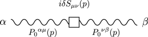
Figure 1: Lorentz-violating propagator insertion. The wavy lines represent the usual Lorentz-symmetric Stueckelberg propagator given by Eq. (28). The square box denotes the the Lorentz-breaking insertion determined by Eq. (30).

VI Summary

In this work, we have employed the Stueckelberg method to introduce a mass term into the full SME’s photon sector in an $R_{\xi}$-type gauge, such that the usual smooth behavior of the model in the $m\to 0$ limit is maintained. We have discussed the resulting equations of motion in the presence of external conserved sources, and studied their solutions. Our results include the exact dispersion relation and propagator for free massive photons incorporating all possible Lorentz-violating, translation- and gauge-invariant Lagrangian contributions at arbitrary mass dimension. From these exact results, we have extracted leading-order expressions for the dispersion-relation roots and the propagator. The method for obtaining the roots is recursive; it also yields higher-order corrections, and it naturally separates the physical solutions from spurious modes arising from higher-derivative terms in the Lagrangian. Finally, we have verified that the number of physical modes is three, as expected for a massive vector particle.

Our results are intended primarily to provide a flexible tool for regularizing infrared divergences in quantum electrodynamics in the presence of general Lorentz violation. A follow-up work in this context is already in preparation CLP . In addition, our expressions for the dispersion relation and propagator also hold for the quadratic part of the SME’s heavy-boson sector, and are therefore expected to find applications in theoretical and phenomenological studies of electroweak physics with Lorentz breaking. In the $m\to 0$ limit, our results yield the previously unknown massless photon propagator in the full SME, a quantity indispensable for many Lorentz-symmetry investigations in electrodynamics.

Appendix A Matrix relations

This appendix provides a collection of various textbook linear-algebra results necessary for the line of reasoning in the main text. For completeness, we have sketched the derivation of these results.

Consider an arbitrary $4\times 4$ matrix $\Lambda$ and denote its four (not necessarily distinct) eigenvalues by $\lambda_{j}$, where $j=1,\ldots,4$. The characteristic polynomial $C(\lambda)$ of $\Lambda$ can then be expressed as

$$C(\lambda)=(\lambda-\lambda_{1})(\lambda-\lambda_{2})(\lambda-\lambda_{3})(\lambda-\lambda_{4})\,.$$ (32)

By the Cayley–Hamilton theorem, the matrix $\Lambda$ must satisfy $C(\Lambda)=0$. Expanding the right-hand side of Eq. (32) and replacing $\lambda\to\Lambda$ then yields

$$\Lambda^{4}+c_{3}\Lambda^{3}+c_{2}\Lambda^{2}+c_{1}\Lambda+c_{0}\openone=0\,,$$ (33)

where the coefficients $c_{j}$ are given by

$${}c_{0}\! = \!\lambda_{1}\lambda_{2}\lambda_{3}\lambda_{4}\,,$$

$${}c_{1}\! = \!-\lambda_{1}\lambda_{2}\lambda_{3}-\lambda_{1}\lambda_{4}\lambda_{3}-\lambda_{2}\lambda_{4}\lambda_{3}-\lambda_{1}\lambda_{2}\lambda_{4}\,,$$

$${}c_{2}\! = \!\lambda_{1}\lambda_{2}+\lambda_{3}\lambda_{2}+\lambda_{4}\lambda_{2}+\lambda_{1}\lambda_{3}+\lambda_{1}\lambda_{4}+\lambda_{3}\lambda_{4}\,,$$

$${}c_{3}\! = \!-\lambda_{1}-\lambda_{2}-\lambda_{3}-\lambda_{4}\,.$$ (34)

The next task is to express the $c_{j}$ in terms of manifestly component-independent expressions involving $\Lambda$. To this end, we transform $\Lambda$ to its Jordan normal form $\Lambda^{\prime}=M^{-1}\Lambda M$, where $M$ is an appropriate $4\times 4$ matrix. Since such a similarity transformation leaves unchanged the eigenvalues, it is straightforward to verify that

$$\det(\Lambda^{\prime})\! = \!\lambda_{1}\lambda_{2}\lambda_{3}\lambda_{4}\,,$$

$$\textrm{Tr}(\Lambda^{\prime n})\! = \!\lambda_{1}^{n}+\lambda_{2}^{n}+\lambda_{3}^{n}+\lambda_{4}^{n}\,,$$ (35)

where $n\in\mathbb{N}$. Inspection now establishes that

$$c_{0}\! = \!\det(\Lambda^{\prime})\,,$$

$$c_{1}\! = \!\tfrac{1}{2}\textrm{Tr}(\Lambda^{\prime 2})\textrm{Tr}(\Lambda^{\prime})-\tfrac{1}{3}\textrm{Tr}(\Lambda^{\prime 3})-\tfrac{1}{6}\textrm{Tr}(\Lambda^{\prime})^{3}\,,$$

$$c_{2}\! = \!{\textstyle\frac{1}{2}}\left[\textrm{Tr}(\Lambda^{\prime})^{2}-\textrm{Tr}(\Lambda^{\prime 2})\right]\,,$$

$$c_{3}\! = \!-\textrm{Tr}(\Lambda^{\prime})\,.$$ (36)

Since both the determinant as well as the trace of a square matrix remain unchanged under similarity transformations, the relations in Eqs. (A) and (A) hold, in fact, also for our original $4\times 4$ matrix $\Lambda$. Employing these results in Eq. (33) gives

$$\Lambda^{4}-[\Lambda]\,\Lambda^{3}+\tfrac{1}{2}\left([\Lambda]^{2}-[\Lambda^{2}]\right)\Lambda^{2}\\ {}+\left(\tfrac{1}{2}[\Lambda^{2}][\Lambda]-\tfrac{1}{3}[\Lambda^{3}]-\tfrac{1}{6}[\Lambda]^{3}\right)\Lambda+\det(\Lambda)\openone=0\,.$$ (37)

Here, we have abbreviated the matrix trace by square brackets. This result establishes that the set of matrices $\{\openone,\Lambda,\Lambda^{2},\Lambda^{3},\Lambda^{4}\}$ is linearly dependent.

Equation (37) can be employed to determine further relations involving the $4\times 4$ matrix $\Lambda$. For example, taking the trace of Eq. (37) yields the expression

$$\det(\Lambda)\! = \!\tfrac{1}{24}[\Lambda]^{4}-\tfrac{1}{4}[\Lambda^{4}]+\tfrac{1}{8}[\Lambda^{2}]^{2}$$ (38)

$$\!{}+\tfrac{1}{3}[\Lambda][\Lambda^{3}]-\tfrac{1}{4}[\Lambda]^{2}[\Lambda^{2}]$$

for the determinant of $\Lambda$. Another relation can be obtained by multiplying Eq. (37) with the inverse matrix $\Lambda^{-1}$. The resulting equation can then be solved for $\Lambda^{-1}$:

$${}\Lambda^{-1}=\frac{1}{\det(\Lambda)}\left(\tfrac{1}{3}[\Lambda^{3}]\openone+\tfrac{1}{6}[\Lambda]^{3}\openone-\tfrac{1}{2}[\Lambda^{2}][\Lambda]\openone\right.\\ \left.{}-\tfrac{1}{2}[\Lambda]^{2}\Lambda+\tfrac{1}{2}[\Lambda^{2}]\Lambda+[\Lambda]\,\Lambda^{2}-\Lambda^{3}\right).$$ (39)

In Eqs. (38) and (39) we have again abbreviated the matrix trace by square brackets.

Appendix B Dispersion relation

To present $r_{0}$, $r_{1}$, and $r_{2}$ appearing in the physical dispersion relation (20), we introduce the following more efficient notation. We suppress the $AF$ subscript on $\hat{k}_{AF}$ and drop the caret:

$$(\hat{k}_{AF})^{\mu}\equiv k^{\mu}\,.$$ (40)

It is also convenient to extract the traceless part $\hat{\underline{G}}{}^{\mu\nu}$ from the full $\hat{G}^{\mu\nu}$:

$$\hat{\underline{G}}{}^{\mu\nu}\equiv\hat{G}^{\mu\nu}-\tfrac{1}{4}[\hat{G}]\eta^{\mu\nu}\,.$$ (41)

Here, we have again denoted the matrix trace by square brackets $[\hat{G}]\equiv\hat{G}^{\mu}_{\mu}$. Inspection of our model Lagrangian (10) reveals that for the photon the decomposition (41) can be implemented by the replacements

$$\hat{G}^{\mu\nu} \to \underline{\hat{G}}{}^{\mu\nu}$$

$$m \to \hat{m}\equiv m\big{(}1+\tfrac{1}{4}[\hat{G}]\big{)}$$

$$\xi^{-1} \to \hat{\xi}^{-1}\equiv\xi^{-1}\big{(}1+\tfrac{1}{4}[\hat{G}]\big{)}^{2}\,,$$ (42)

where it is understood that $\hat{\xi}^{-1/2}$ has to be placed at the appropriate position in the gauge-fixing term. We also remind the reader that we denote the contraction of a 4-vector with a symmetric 2-tensor by writing the vector as a superscript or a subscript on the tensor: for example $(\underline{\hat{G}}{}^{2}){}^{k}_{p}\equiv\underline{\hat{G}}{}^{\alpha}_{\beta}\underline{\hat{G}}{}^{\beta}_{\gamma}\,p_{\alpha}(\hat{k}_{AF})^{\gamma}$, etc.

With this notation, the $r$ coefficients in the physical dispersion relation (20) take the following form:

$${}r_{0}\! = \!\tfrac{4}{3}[\hat{K}]^{3}+\tfrac{8}{3}[\hat{K}^{3}]-4[\hat{K}][\hat{K}^{2}]+8\hat{m}^{2}\hat{K}^{k}_{k}+2[\hat{K}]^{2}\underline{\hat{G}}{}^{p}_{p}-2[\hat{K}^{2}]\underline{\hat{G}}{}^{p}_{p}-4(k\cdot p)^{2}\underline{\hat{G}}{}^{p}_{p}-4\hat{m}^{2}[\underline{\hat{G}}{}\hat{K}^{2}]+4\hat{m}^{2}[\hat{K}][\underline{\hat{G}}{}\hat{K}]$$

$$\!{}-2\hat{m}^{2}(\underline{\hat{G}}{}\hat{K}\underline{\hat{G}}{})^{p}_{p}+2\hat{m}^{2}[\hat{K}](\underline{\hat{G}}{}^{2})^{p}_{p}+2\hat{m}^{2}[\underline{\hat{G}}{}\hat{K}]\underline{\hat{G}}{}^{p}_{p}+8\hat{m}^{2}(k\cdot p)\underline{\hat{G}}{}^{k}_{p}+2\hat{m}^{4}[\underline{\hat{G}}{}^{2}\hat{K}]-\hat{m}^{4}[\hat{K}][\underline{\hat{G}}{}^{2}]-4\hat{m}^{4}\underline{\hat{G}}{}^{k}_{k}$$

$$\!{}+\hat{m}^{4}(\underline{\hat{G}}{}^{3})^{p}_{p}-\tfrac{1}{2}\hat{m}^{4}[\underline{\hat{G}}{}^{2}]\underline{\hat{G}}{}^{p}_{p}-\tfrac{1}{3}\hat{m}^{6}[\underline{\hat{G}}{}^{3}]-8[\underline{\hat{G}}{}\hat{K}^{3}]+8[\hat{K}][\underline{\hat{G}}{}\hat{K}^{2}]-4[\hat{K}]^{2}[\underline{\hat{G}}{}\hat{K}]+4[\hat{K}^{2}][\underline{\hat{G}}{}\hat{K}]+8\hat{K}^{k}_{k}\underline{\hat{G}}{}^{p}_{p}$$

$$\!{}+4\hat{m}^{2}[\underline{\hat{G}}{}^{2}\hat{K}^{2}]-2\hat{m}^{2}[\underline{\hat{G}}{}\hat{K}]^{2}+2\hat{m}^{2}[(\underline{\hat{G}}{}\hat{K})^{2}]+\hat{m}^{2}[\hat{K}]^{2}[\underline{\hat{G}}{}^{2}]-\hat{m}^{2}[\hat{K}^{2}][\underline{\hat{G}}{}^{2}]-4\hat{m}^{2}[\hat{K}][\underline{\hat{G}}{}^{2}\hat{K}]+4\hat{m}^{2}(\underline{\hat{G}}{}^{k}_{p})^{2}$$

$$\!{}-4\hat{m}^{2}\underline{\hat{G}}{}^{k}_{k}\underline{\hat{G}}{}^{p}_{p}-2\hat{m}^{4}[\underline{\hat{G}}{}^{3}\hat{K}]+\hat{m}^{4}[\underline{\hat{G}}{}\hat{K}][\underline{\hat{G}}{}^{2}]+\tfrac{2}{3}\hat{m}^{4}[\hat{K}][\underline{\hat{G}}{}^{3}]-\tfrac{1}{8}\hat{m}^{6}[\underline{\hat{G}}{}^{2}]^{2}+\tfrac{1}{4}\hat{m}^{6}[\underline{\hat{G}}{}^{4}]\,,$$

$${}r_{1}\! = \!2[\hat{K}]^{2}-2[\hat{K}^{2}]-4(k\cdot p)^{2}+4\hat{m}^{2}k^{2}+2[\hat{K}]\underline{\hat{G}}{}^{p}_{p}+2\hat{m}^{2}[\underline{\hat{G}}{}\hat{K}]+\hat{m}^{2}(\underline{\hat{G}}{}^{2})^{p}_{p}-\tfrac{1}{2}\hat{m}^{4}[\underline{\hat{G}}{}^{2}]+8\hat{K}^{k}_{k}+4k^{2}\underline{\hat{G}}{}^{p}_{p}-4\hat{m}^{2}\underline{\hat{G}}{}^{k}_{k}\,,$$

$${}r_{2}\! = \!2[\hat{K}]+\underline{\hat{G}}{}^{p}_{p}+4k^{2}\,.$$ (43)

The above dispersion relation can be shown to reduce in the appropriate limit to mass-dimension three results quoted in Ref. AACGS .

To determine the quantities $R_{j}$ appearing in Eq. (22), we apply the usual Tschirnhaus-type transformation for cubic equations to Expression (20). This yields the equivalent depressed form of the physical dispersion relation $Q=0$:

$$\left(p^{2}-\hat{m}^{2}+\tfrac{2}{3}[\hat{K}]+\tfrac{1}{3}\underline{\hat{G}}{}^{p}_{p}+\tfrac{4}{3}k^{2}\right)^{3}+s_{1}\left(p^{2}-\hat{m}^{2}+\tfrac{2}{3}[\hat{K}]+\tfrac{1}{3}\underline{\hat{G}}{}^{p}_{p}+\tfrac{4}{3}k^{2}\right)+s_{0}=0\,,$$ (44)

where coefficients $s_{0}$ and $s_{1}$ are given by

$${}s_{0}\! = \!\tfrac{16}{27}[\hat{K}]^{3}+\tfrac{8}{3}[\hat{K}^{3}]-\tfrac{8}{3}[\hat{K}][\hat{K}^{2}]+\tfrac{8}{3}(k\cdot p)^{2}[\hat{K}]+8\hat{m}^{2}\hat{K}^{k}_{k}-\tfrac{8}{3}\hat{m}^{2}k^{2}[\hat{K}]+\tfrac{8}{9}[\hat{K}]^{2}\underline{\hat{G}}{}^{p}_{p}-\tfrac{4}{3}[\hat{K}^{2}]\underline{\hat{G}}{}^{p}_{p}-\tfrac{2}{9}[\hat{K}](\underline{\hat{G}}{}^{p}_{p})^{2}\qquad$$

$$\!{}-\tfrac{8}{3}(k\cdot p)^{2}\underline{\hat{G}}{}^{p}_{p}+\tfrac{2}{27}(\underline{\hat{G}}{}^{p}_{p})^{3}-4\hat{m}^{2}[\underline{\hat{G}}{}\hat{K}^{2}]+\tfrac{8}{3}\hat{m}^{2}[\hat{K}][\underline{\hat{G}}{}\hat{K}]-2\hat{m}^{2}(\underline{\hat{G}}{}\hat{K}\underline{\hat{G}}{})^{p}_{p}+\tfrac{4}{3}\hat{m}^{2}[\hat{K}](\underline{\hat{G}}{}^{2})^{p}_{p}+\tfrac{4}{3}\hat{m}^{2}[\underline{\hat{G}}{}\hat{K}]\underline{\hat{G}}{}^{p}_{p}$$

$$\!{}-\tfrac{1}{3}\hat{m}^{2}\underline{\hat{G}}{}^{p}_{p}(\underline{\hat{G}}{}^{2})^{p}_{p}-\tfrac{4}{3}\hat{m}^{2}k^{2}\underline{\hat{G}}{}^{p}_{p}+8\hat{m}^{2}(k\cdot p)\underline{\hat{G}}{}^{k}_{p}+2\hat{m}^{4}[\underline{\hat{G}}{}^{2}\hat{K}]-\tfrac{2}{3}\hat{m}^{4}[\hat{K}][\underline{\hat{G}}{}^{2}]-4\hat{m}^{4}\underline{\hat{G}}{}^{k}_{k}-\tfrac{1}{3}\hat{m}^{4}[\underline{\hat{G}}{}^{2}]\underline{\hat{G}}{}^{p}_{p}$$

$$\!{}+\hat{m}^{4}(\underline{\hat{G}}{}^{3})^{p}_{p}-\tfrac{1}{3}\hat{m}^{6}[\underline{\hat{G}}{}^{3}]+\tfrac{8}{9}k^{2}[\hat{K}]^{2}+\tfrac{8}{3}k^{2}[\hat{K}^{2}]-\tfrac{16}{3}[\hat{K}]\hat{K}^{k}_{k}+\tfrac{16}{3}k^{2}(k\cdot p)^{2}-\tfrac{4}{9}k^{2}(\underline{\hat{G}}{}^{p}_{p})^{2}+8[\hat{K}][\underline{\hat{G}}{}\hat{K}^{2}]$$

$$\!{}-8[\underline{\hat{G}}{}\hat{K}^{3}]-4[\hat{K}]^{2}[\underline{\hat{G}}{}\hat{K}]+4[\hat{K}^{2}][\underline{\hat{G}}{}\hat{K}]+\tfrac{16}{3}\hat{K}^{k}_{k}\underline{\hat{G}}{}^{p}_{p}-\tfrac{16}{9}k^{2}[\hat{K}]\underline{\hat{G}}{}^{p}_{p}-4\hat{m}^{2}[\hat{K}][\underline{\hat{G}}{}^{2}\hat{K}]+2\hat{m}^{2}[(\underline{\hat{G}}{}\hat{K})^{2}]$$

$$\!{}+4\hat{m}^{2}[\underline{\hat{G}}{}^{2}\hat{K}^{2}]-2\hat{m}^{2}[\underline{\hat{G}}{}\hat{K}]^{2}+\hat{m}^{2}[\hat{K}]^{2}[\underline{\hat{G}}{}^{2}]-\hat{m}^{2}[\hat{K}^{2}][\underline{\hat{G}}{}^{2}]-\tfrac{8}{3}\hat{m}^{2}k^{2}[\underline{\hat{G}}{}\hat{K}]+4\hat{m}^{2}(\underline{\hat{G}}{}^{k}_{p})^{2}-\tfrac{8}{3}\hat{m}^{2}\underline{\hat{G}}{}^{k}_{k}\underline{\hat{G}}{}^{p}_{p}$$

$$\!{}-\tfrac{16}{3}\hat{m}^{2}k^{4}+\tfrac{8}{3}\hat{m}^{2}[\hat{K}]\underline{\hat{G}}{}^{k}_{k}-\tfrac{4}{3}\hat{m}^{2}k^{2}(\underline{\hat{G}}{}^{2})^{p}_{p}-2\hat{m}^{4}[\underline{\hat{G}}{}^{3}\hat{K}]+\hat{m}^{4}[\underline{\hat{G}}{}\hat{K}][\underline{\hat{G}}{}^{2}]+\tfrac{2}{3}\hat{m}^{4}[\hat{K}][\underline{\hat{G}}{}^{3}]+\tfrac{2}{3}\hat{m}^{4}k^{2}[\underline{\hat{G}}{}^{2}]$$

$$\!{}-\tfrac{1}{8}\hat{m}^{6}[\underline{\hat{G}}{}^{2}]^{2}+\tfrac{1}{4}\hat{m}^{6}[\underline{\hat{G}}{}^{4}]+\tfrac{64}{9}k^{4}[\hat{K}]-\tfrac{32}{3}k^{2}\hat{K}^{k}_{k}-\tfrac{16}{9}k^{4}\underline{\hat{G}}{}^{p}_{p}+\tfrac{16}{3}\hat{m}^{2}k^{2}\underline{\hat{G}}{}^{k}_{k}+\tfrac{128}{27}k^{6}\,,$$

$${}s_{1}\! = \!\tfrac{2}{3}[\hat{K}]^{2}-2[\hat{K}^{2}]-4(k\cdot p)^{2}+4\hat{m}^{2}k^{2}+\tfrac{2}{3}[\hat{K}]\underline{\hat{G}}{}^{p}_{p}-\tfrac{1}{3}(\underline{\hat{G}}{}^{p}_{p})^{2}+2\hat{m}^{2}[\underline{\hat{G}}{}\hat{K}]+\hat{m}^{2}(\underline{\hat{G}}{}^{2})^{p}_{p}-\tfrac{1}{2}\hat{m}^{4}[\underline{\hat{G}}{}^{2}]+8\hat{K}^{k}_{k}$$ (45)

$$\!{}-\tfrac{16}{3}k^{2}[\hat{K}]+\tfrac{4}{3}k^{2}\underline{\hat{G}}{}^{p}_{p}-4\hat{m}^{2}\underline{\hat{G}}{}^{k}_{k}-\tfrac{16}{3}k^{4}\,.$$

With $s_{0}$ and $s_{1}$ at hand, the usual formulae for the roots of a cubic determine explicit expressions for the $R_{j}$ quantities. These expressions can then be used for the iteration Eq. (25): Suppose we want to calculate the first-order frequencies from the zeroth-order solution $(\sqrt{\vec{p}^{\,2}+m^{2}},\vec{p})$, which corresponds to the first iteration step in Eq. (25). With $(\sqrt{\vec{p}^{\,2}+m^{2}},\vec{p})$ and Eqs. (B), we can in principle check the sign of the discriminant $4s_{1}{}^{3}+27s_{0}{}^{2}$, at least to leading order. A positive discriminant is associated with complex-valued $R_{j}$, which would appear to lead to unphysical roots. We therefore take the discriminant to be non-positive in what follows. The $R_{j}$ can then be expressed trigonometrically:

$$R_{j}=2\sqrt{-\frac{s_{1}}{3}}\cos\left[\frac{1}{3}\cos^{-1}\left(\frac{3s_{0}}{2s_{1}}\sqrt{-\frac{3}{s_{1}}}\right)-\frac{2\pi}{3}j\right]-\tfrac{2}{3}[\hat{K}]-\tfrac{1}{3}\underline{\hat{G}}{}^{p}_{p}-\tfrac{4}{3}k^{2}\,,\quad j\in\{1,2,3\}\,.$$ (46)

These explicit $R_{j}$ can now, for example, be employed in the context of Eq. (25).

We remark that for the special case of a vanishing discriminant, Eq. (46) determines a multiple root, so that at least two physical excitations propagate without birefringence. We also note that for non-positive discriminant the argument of the cosine function in Eq. (46) is real, and its magnitude therefore remains bounded by one. The limit of zero Lorentz violation is then determined by $s_{1}$, $[\hat{K}]$, $\underline{\hat{G}}{}^{p}_{p}$, and $k^{2}$. These coefficients will generically be momentum dependent. In particular, the zero components for the unphysical solutions may diverge in this limit, so that the corresponding behavior of the $R_{j}$ is unclear a priori. However, for the physical solutions the plane-wave frequencies must remain bounded because they are defined to approach the conventional expressions in the Lorentz-symmetric limit. For vanishing Lorentz breaking, the physical $R_{j}$ are therefore seen to approach zero, as required by self-consistency.

Appendix C Discrete symmetries

An interesting question concerns the number of independent plane-wave solutions. Some insight into this issue can be gained by investigating discrete symmetries of both the plane-wave polarization vectors and the dispersion relation (19).

Since the Lagrangian (10) is real, the momentum-space Stueckelberg operator must be hermitian

$$S^{\mu\nu}(p)^{*}=S^{\nu\mu}(p)\,,$$ (47)

which can also be established directly by inspection of Eq. (17). Next, we consider $S^{\mu\nu}(p)$ under $p\to-p$. Only the $\hat{k}_{AF}$ piece reverses its sign because it is odd in $p$. All other terms are $p$ even and remain unchanged. We also need the behavior of $S^{\mu\nu}(p)$ under complex conjugation. Since the position-space Stueckelberg operator is purely real, complex-valued contributions to the momentum-space $S^{\mu\nu}(p)$ can only arise from the Fourier replacement $\partial\to-ip$. We will focus on real-valued plane-wave momenta $p$ since otherwise an interpretation as a propagating solution is difficult. It then follows that the $p$-odd $\hat{k}_{AF}$ term is purely imaginary, while all other terms are even in $p$ even and thus real. Complex conjugation of $S^{\mu\nu}(p)$ therefore only changes the sign of its $\hat{k}_{AF}$ piece. It thus becomes evident that the momentum-space Stueckelberg operator is left unaffected under the combination of the two operations:

$${}S^{\mu\nu}(+p,+\hat{k}_{AF},\hat{k}_{F},\hat{G}) = S^{\mu\nu}(-p,+\hat{k}_{AF},\hat{k}_{F},\hat{G})^{*}$$ (48)

$$= S^{\nu\mu}(-p,+\hat{k}_{AF},\hat{k}_{F},\hat{G})\,,$$

where the Hermiticity of $S^{\mu\nu}$ has been used. Since any determinant is invariant under transposition, we find

$$\det S(+p,\hat{k}_{AF},\hat{k}_{F},\hat{G})=\det S(-p,\hat{k}_{AF},\hat{k}_{F},\hat{G})\,,$$ (49)

i.e., $p\to-p$ represents a discrete symmetry of the dispersion relation. This invariance also becomes clear when Eqs. (19), (20), and (B) are combined.

Continuing our analysis in a concordant frame caus , we fix a wave 3-vector $\vec{p}$ and imagine solving the dispersion relation (19). Following the reasoning presented in Sec. V, we can eliminate the spurious Ostrogradski modes and focus on the six physical branches of the dispersion-relation solution with exact $\omega^{j,\pm}_{\vec{p}}$. In these expressions, the $\pm$ label must correspond to the sign of the solution, a property that follows immediately from the required proximity to the Lorentz-symmetric sheets fn3 . Without loss of generality, we now consider the specific plane-wave 4-momentum with positive energy $(p_{+}^{j})^{\mu}\equiv(\omega^{j,+}_{-\vec{p}},-\vec{p})$. The $p\to-p$ symmetry of the dispersion relation implies that $(p_{-}^{j})^{\mu}\equiv(-\omega^{j,+}_{-\vec{p}},\vec{p})$ also represents a solution, but one with negative frequency. Moreover, this solution must be physical: since $p_{+}^{j}$ is close to the conventional positive sheet, $p_{-}^{j}$ must be a perturbation of the negative sheet. With a suitable selection of the $j$ labels, we may therefore conclude $\omega^{j,-}_{\vec{p}}=-\omega^{j,+}_{-\vec{p}}$. In summary, the set of physical plane-wave momenta is given by

$$\left\{(p_{+}^{j})^{\mu}=(\omega_{\vec{p}}^{j,+},\vec{p})\,\,,\,\,\,\,(p_{-}^{j})^{\mu}=(-\omega_{-\vec{p}}^{j,+},\vec{p})\right\},$$ (50)

and is thus determined entirely by the expressions for the three positive-frequency solutions $\omega^{j,+}_{\vec{p}}$.

In addition to the plane-wave momenta $(p_{\pm}^{j})^{\mu}$, the associated polarization vectors $(\varepsilon^{j}_{\pm})^{\mu}(\vec{p})$ are needed to construct a plane wave. Given the $\varepsilon^{j}_{+}(\vec{p})$ associated with the positive-frequency roots, we can construct the remaining negative-frequency $\varepsilon^{j}_{-}(\vec{p})$ as follows. Up to normalization, the polarization vectors are by definition in the kernel of the Stueckelberg operator: $S(\omega^{j,\pm}_{\vec{p}},\vec{p})\,\varepsilon^{j}_{\pm}(\vec{p})=0$. This definition contains $S(\omega^{j,+}_{-\vec{p}},-\vec{p})\,\varepsilon^{j}_{+}(-\vec{p})=0$ as a special case. Complex conjugation combined with Eq. (48) then yields $S(-\omega^{j,+}_{-\vec{p}},\vec{p})\,\varepsilon^{j}_{+}{}^{*}(-\vec{p})=0$. Together with the plane-wave momentum property (50), this equation is identified as the defining relation for $\varepsilon^{j}_{-}(\vec{p})$. Using suitable normalizations, we arrive at

$$(\varepsilon^{j}_{-})^{\mu}(\vec{p})=(\varepsilon^{j}_{+}{}^{*})^{\mu}(-\vec{p})\,.$$ (51)

We remark that this relation continues to hold for dispersion-relation roots with higher multiplicities when the bases of $\textrm{Ker}\,S(-\omega^{j,+}_{-\vec{p}},\vec{p})$ are chosen appropriately.

An arbitrary, free, real-valued, physical solution $A^{\mu}(x)$ can be represented by the following Fourier superposition of plane waves fn4 :

$$A^{\mu}(x) = \int\!\!\frac{d^{3}\vec{p}}{(2\pi)^{3}}\sum_{j=1}^{3}\left[a^{j}_{+}(\vec{p})\,(\varepsilon^{j}_{+})^{\mu}(\vec{p})\,e^{-ip^{j}_{+}\cdot x}\right.$$ (52)

$$\left.{}\hskip 31.29802pt+a^{j}_{-}(\vec{p})\,(\varepsilon^{j}_{-})^{\mu}(\vec{p})\,e^{-ip^{j}_{-}\cdot x}\right]+\textrm{c.c.}$$

This expression suggests that six Fourier coefficients $\{a^{j}_{+}(\vec{p}),a^{j}_{-}(\vec{p})\}$ with $j=1,2,3$ must be specified independently to determine a general solution. However, a change of integration variable $\vec{p}\to-\vec{p}$ in the expression associated with the negative-frequency solutions together with Eqs. (50) and (51) yields

$$A^{\mu}(x)=\int\!\!\frac{d^{3}\vec{p}}{(2\pi)^{3}}\sum_{j=1}^{3}b^{j}(\vec{p})\,(\varepsilon^{j}_{+})^{\mu}(\vec{p})\,e^{-ip^{j}_{+}\cdot x}+\textrm{c.c.},$$ (53)

where we have defined $b^{j}(\vec{p})\equiv a^{j}_{+}(\vec{p})+a^{j}_{-}{}^{*}(-\vec{p})$. This establishes that the six physical dispersion-relation roots are associated with three degrees of freedom.

Appendix D Massless limit

In the context of regularizing infrared divergences in quantum-field perturbation theory, the massless limit of our Lorentz-violating Stueckelberg model is of particular importance. The photon mass was introduced into our Lagrangian via the Stueckelberg method, which ensures the proper behavior in this limit. Nevertheless, it is interesting to study explicitly the dispersion relation and the propagator of our model for vanishing $m$, for example, to compare with previous results for massless Lorentz-violating photons.

We begin by defining the contraction

$${}\hat{I}\equiv\epsilon_{\alpha\beta\gamma\delta}\epsilon_{\kappa\lambda\mu\nu}p_{\rho}p_{\sigma}p_{\tau}p_{\iota}(\hat{k}_{F})^{\alpha\beta\kappa\rho}(\hat{k}_{F})^{\lambda\sigma\tau\gamma}(\hat{k}_{F})^{\iota\delta\mu\nu}$$ (54)

of the Lorentz-violating $\hat{k}_{F}$. One can show that the coordinate scalar $\hat{I}$ obeys the following identities:

$$\tfrac{1}{12}\,\hat{I}\,\underline{\hat{G}}{}^{p}_{p} = 2[\underline{\hat{G}}{}\hat{K}^{3}]-2[\underline{\hat{G}}{}\hat{K}^{2}][\hat{K}]+[\underline{\hat{G}}{}\hat{K}]\big{(}[\hat{K}]^{2}-[\hat{K}^{2}]\big{)}$$

$$\tfrac{1}{4}\,\hat{I}\,p^{2} = 3[\hat{K}][\hat{K}^{2}]-[\hat{K}]^{3}-2[\hat{K}^{3}]\,.\qquad\qquad\qquad\qquad\quad$$ (55)

With these identities, the full massless dispersion relation (19) can be cast into the form

$$\hat{\xi}\det S = (\hat{\eta}^{\mu\nu}p_{\mu}p_{\nu})^{2}\Big{(}p^{4}+2[\hat{K}]p^{2}+8\hat{K}^{k}_{k}-\tfrac{1}{3}\hat{I}$$ (56)

$${}-4(k\cdot p)^{2}+4k^{2}p^{2}+2[\hat{K}]^{2}-2[\hat{K}^{2}]\Big{)}\,.\qquad$$

It thus becomes apparent that in the massless limit the expression $(\hat{\eta}^{\mu\nu}p_{\mu}p_{\nu})$ can be factored out of $Q$.

The next step is to identify the physical part of the massless dispersion relation (56). Clearly, one of the $(\hat{\eta}^{\mu\nu}p_{\mu}p_{\nu})$ factors originates from the auxiliary mode and remains unphysical. To gain insight into the other factors, it is instructive to recall the model Lagrangian (10). In the zero-mass limit, $\hat{G}$ enters the equations of motion for the photon only via the gauge-fixing term ${\cal L}_{\textrm{g.f.}}$ and should therefore not lead to observable effects. It then follows that the second $(\hat{\eta}^{\mu\nu}p_{\mu}p_{\nu})$ factor must also be unphysical because it contains $\hat{\eta}=\eta+\hat{G}$. We conclude that the last factor in Eq. (56), which is free of $\hat{G}$, governs the physical excitations for $m=0$. This factor is in agreement with the general photon dispersion relation given in Ref. PhotonSME , as required by consistency.

The exact massive propagator (21) as well as its leading-order approximation (26) exhibit six physical poles that must be encircled by the integration contours. The above argument identifies those two of these six poles that should become unphysical in the massless case. The question then arises as to whether the unphysical character of these two modes is reflected in the pole structure of the propagator in the $m\to 0$ limit. This may be established by demonstrating that the $(\hat{\eta}^{\mu\nu}p_{\mu}p_{\nu})$ factor in the denominator of the propagator is cancelled by a corresponding $(\hat{\eta}^{\mu\nu}p_{\mu}p_{\nu})$ factor in the numerator for vanishing mass. An investigation of this cancellation for the exact expression (21) would be interesting but lies outside the scope of the present work. We instead focus on the on the leading-order piece (26) of the propagator, which is appropriate for the majority of practical applications.

In the discussion of the leading-order propagator (26), it was already mentioned that the $(1-\xi)$ contribution in the second line leaves unaffected observable quantities. We may therefore focus on the physical contribution contained in the first line of Eq. (26). In the $m\to 0$ limit, the numerator $-iN^{\mu\nu}$ of this first piece has the form

$$N^{\mu\nu} = p^{2}\big{(}2[\hat{K}]\eta^{\mu\nu}-2\hat{K}^{\mu\nu}+2i\hat{\cal E}^{\mu\nu}+p^{\mu}\hat{G}^{\nu}_{p}+p^{\nu}\hat{G}^{\mu}_{p}\big{)}$$ (57)

$${}+p^{2}\big{(}p^{2}+\hat{G}^{p}_{p}\big{)}\eta^{\mu\nu}\,.\qquad\qquad\qquad\qquad\qquad\qquad\;$$

The $\eta^{\mu\nu}$ term in the second line of the above Eq. (57) contains the factor $p^{2}+\hat{G}^{p}_{p}=\hat{\eta}^{\mu\nu}p_{\mu}p_{\nu}$. All terms in the first line represent leading-order corrections, which remain unaffected by the addition of higher-order Lorentz-violating terms. A judicious choice for such higher-order contributions is $p^{2}\to p^{2}+\hat{G}^{p}_{p}=\hat{\eta}^{\mu\nu}p_{\mu}p_{\nu}$ in the overall $p^{2}$ factor. It thus becomes evident that in the physical piece of the leading-order propagator, the factor $(\hat{\eta}^{\mu\nu}p_{\mu}p_{\nu})$ appears in both the numerator and the denominator and therefore cancels. We conclude that the poles that become unphysical in the massless limit disappear from the propagator, at least to leading order.

Since $\hat{G}$ arises in the massless case solely from the gauge-fixing term, measurable quantities are necessarily free of $\hat{G}$, even though $p^{\mu}\hat{G}^{\nu}_{p}$ and $p^{\nu}\hat{G}^{\mu}_{p}$ terms still appear in the numerator of the propagator (26) and, equivalently, in the propagator insertion (30). When the propagator is contracted with a conserved current $\bar{\jmath}^{\,\nu}$, $\hat{G}$ independence can be seen explicitly as follows. For the $p^{\mu}\hat{G}^{\nu}_{p}$ term, such a contraction yields an expression proportional to $p^{\mu}$, which is pure gauge and can therefore not lead to observable effects. For the $p^{\nu}\hat{G}^{\mu}_{p}$ term, the contraction produces an overall $p\cdot\bar{\jmath}$, which vanishes due to current conservation. It is thus clear that $\hat{G}$ is indeed unobservable in this context, as expected.

References

- (1) V.A. Kostelecký and N. Russell, Rev. Mod. Phys. 83, 11 (2011).
- (2) See, e.g., V.A. Kostelecký and S. Samuel, Phys. Rev. D 39, 683 (1989); V.A. Kostelecký and R. Potting, Nucl. Phys. B 359, 545 (1991); J. Alfaro, H.A. Morales-Técotl, and L.F. Urrutia, Phys. Rev. Lett. 84, 2318 (2000); S.M. Carroll et al., Phys. Rev. Lett. 87, 141601 (2001); J.D. Bjorken, Phys. Rev. D 67, 043508 (2003); V.A. Kostelecký, R. Lehnert, and M.J. Perry, Phys. Rev. D 68, 123511 (2003); O. Bertolami et al., Phys. Rev. D 69, 083513 (2004).
- (3) V.A. Kostelecký and R. Potting, Phys. Rev. D 51, 3923 (1995).
- (4) D. Colladay and V.A. Kostelecký, Phys. Rev. D 55, 6760 (1997); Phys. Rev. D 58, 116002 (1998); V.A. Kostelecký, Phys. Rev. D 69, 105009 (2004); V.A. Kostelecký and M. Mewes, arXiv:1112.6395.
- (5) V.A. Kostelecký and R. Lehnert, Phys. Rev. D 63, 065008 (2001).
- (6) V.A. Kostelecký and M. Mewes, Phys. Rev. D 80, 015020 (2009).
- (7) See, e.g., V.A. Kostelecký and M. Mewes, Phys. Rev. Lett. 87, 251304 (2001); Phys. Rev. D 66, 056005 (2002); R. Lehnert, Phys. Rev. D 68, 085003 (2003); R. Lehnert and R. Potting, Phys. Rev. Lett. 93, 110402 (2004); Phys. Rev. D 70, 125010 (2004); B. Altschul, Phys. Rev. D 78, 085018 (2008).
- (8) G. Amelino-Camelia et al., Eur. Phys. J. C 68, 619 (2010); KLOE Collaboration, A. Di Domenico, J. Phys. Conf. Ser. 171, 012008 (2009); BaBar Collaboration, B. Aubert et al., Phys. Rev. Lett. 100, 131802 (2008); FOCUS Collaboration, J.M. Link et al., Phys. Lett. B 556, 7 (2003); KTeV Collaboration, H. Nguyen, hep-ex/0112046; V.A. Kostelecký and R.J. Van Kooten, Phys. Rev. D 82, 101702(R) (2010); V.A. Kostelecký, Phys. Rev. D 64, 076001 (2001); Phys. Rev. D 61, 016002 (1999); Phys. Rev. Lett. 80, 1818 (1998).
- (9) See, e.g., M.A. Hohensee et al., Phys. Rev. Lett. 102, 170402 (2009); Phys. Rev. D 80, 036010 (2009); J.-P. Bocquet et al. [GRAAL Collaboration], Phys. Rev. Lett. 104, 241601 (2010); B. Altschul, Phys. Rev. D 80, 091901 (2009); Phys. Rev. D 84, 076006 (2011).
- (10) H. Müller et al., Phys. Rev. D 68, 116006 (2003); Ch. Eisele et al., Phys. Rev. Lett. 103, 090401 (2009); M.E. Tobar et al., Phys. Rev. D 80, 125024 (2009).
- (11) T. Katori, V.A. Kostelecký, and R. Tayloe,, Phys. Rev. D 74, 105009 (2006); J.S. Díaz, V.A. Kostelecký, and M. Mewes, Phys. Rev. D 80, 076007 (2009); V. Barger et al., Phys. Rev. D 84, 056014 (2011); J.S. Díaz and V.A. Kostelecký, arXiv:1108.1799.
- (12) R. Bluhm, V.A. Kostelecký, and N. Russell, Phys. Rev. D 57, 3932 (1998); H. Dehmelt et al., Phys. Rev. Lett. 83, 4694 (1999); R. Mittleman et al., Phys. Rev. Lett. 83, 2116 (1999); G. Gabrielse et al., Phys. Rev. Lett. 82, 3198 (1999); D. Bear et al., Phys. Rev. Lett. 85, 5038 (2000); P. Wolf et al., Phys. Rev. Lett. 96, 060801 (2006); I. Altarev et al., Phys. Rev. Lett. 103, 081602 (2009); Europhys. Lett. 92, 51001 (2010).
- (13) Q.G. Bailey and V.A. Kostelecký, Phys. Rev. D 74, 045001 (2006); J.B.R. Battat, J.F. Chandler, and C.W. Stubbs, Phys. Rev. Lett. 99, 241103 (2007); H. Müller et al., Phys. Rev. Lett. 100, 031101 (2008); K.Y. Chung et al., Phys. Rev. D 80, 016002 (2009); V.A. Kostelecký and J.D. Tasson, Phys. Rev. Lett. 102, 010402 (2009); Q.G. Bailey, Phys. Rev. D 80, 044004 (2009); V.A. Kostelecký and J.D. Tasson, Phys. Rev. D 83, 016013 (2011); R. Tso and Q.G. Bailey, Phys. Rev. D 84, 085025 (2011).
- (14) O.W. Greenberg, Phys. Rev. Lett. 89, 231602 (2002); R. Lehnert, J. Math. Phys. 45, 3399 (2004); Phys. Rev. D 74, 125001 (2006); A.J. Hariton and R. Lehnert, Phys. Lett. A 367, 11 (2007); V.A. Kostelecký, Phys. Lett. B 701, 137 (2011).
- (15) V.A. Kostelecký and S. Samuel, Phys. Rev. D 40, 1886 (1989); R. Bluhm and V.A. Kostelecký, Phys. Rev. D 71, 065008 (2005); R. Bluhm, S.-H. Fung, and V.A. Kostelecký, Phys. Rev. D 77, 065020 (2008); R. Bluhm et al., Phys. Rev. D 77, 125007 (2008); V.A. Kostelecký and R. Potting, Phys. Rev. D 79, 065018 (2009); J. Alfaro and L.F. Urrutia, Phys. Rev. D 81, 025007 (2010); B. Altschul, Q. G. Bailey, and V.A. Kostelecký, Phys. Rev. D 81, 065028 (2010); C. Armendáriz-Picón, A. Díez-Tejedor, and R. Penco, JHEP 1010, 079 (2010).
- (16) Q.G. Bailey and V.A. Kostelecký, Phys. Rev. D 70, 076006 (2004); R. Lehnert, Rev. Mex. Fís. 56 (6), 469 (2010); Q.G. Bailey, Phys. Rev. D 82, 065012 (2010); V.A. Kostelecký and N. Russell, Phys. Lett. B 693, 443 (2010).
- (17) R. Jackiw and V.A. Kostelecký, Phys. Rev. Lett. 82, 3572 (1999); V.A. Kostelecký, C.D. Lane, and A.G.M. Pickering, Phys. Rev. D 65, 056006 (2002); A.A. Andrianov, P. Giacconi, and R. Soldati, JHEP 0202, 030 (2002); B. Altschul, Phys. Rev. D 69, 125009 (2004); D. Colladay and P. McDonald, Phys. Rev. D 77, 085006 (2008); Phys. Rev. D 79, 125019 (2009).
- (18) J. Alfaro et al., Phys. Lett. B 639, 586 (2006); Int. J. Mod. Phys. A 25, 3271 (2010).
- (19) R.C. Myers and M. Pospelov, Phys. Rev. Lett. 90, 211601 (2003); B. Altschul and V.A. Kostelecký, Phys. Lett. B 628, 106 (2005); C.M. Reyes, L.F. Urrutia, and J.D. Vergara, Phys. Rev. D 78, 125011 (2008); Phys. Lett. B 675, 336 (2009); C.M. Reyes, Phys. Rev. D 82, 125036 (2010); M. Cambiaso and L.F. Urrutia, Phys. Rev. D 82, 101502 (2010).
- (20) D.L. Anderson, M. Sher, and I. Turan, Phys. Rev. D 70, 016001 (2004); E.O. Iltan, Mod. Phys. Lett. A 19, 327 (2004); B. Altschul, Astropart. Phys. 28, 380 (2007).
- (21) E.C.G. Stueckelberg, Helv. Phys. Acta 11, 225 (1938); Helv. Phys. Acta 11, 299 (1938).
- (22) H. Ruegg and M. Ruiz-Altaba, Int. J. Mod. Phys. A 19, 3265 (2004).
- (23) Odd numbers of derivatives would be equivalent to total-divergence terms in the Lagrangian piece (3).
- (24) This may entail a momentum cut-off, which is consistent with our effective-field-theory interpretation.
- (25) B. Altschul, Phys. Rev. D 73, 045004 (2006).
- (26) M.V. Ostrogradski, Mem. Acad. Imp. Sci. St. Petersbourg VI 4, 385 (1850).
- (27) S.M. Carroll, G.B. Field, and R. Jackiw, Phys. Rev. D 41, 1231 (1990); C. Adam and F. R. Klinkhamer, Nucl. Phys. B 607, 247 (2001); R. Casana et al., Phys. Rev. D 80, 125040 (2009); R. Casana et al., Phys. Rev. D 82, 125006 (2010); F.R. Klinkhamer and M. Schreck, Nucl. Phys. B 848, 90 (2011); M. Schreck, arXiv:1111.4182.
- (28) For the photon, becomes unobservable in the massless limit. But without loss of generality, we may take it to be small.
- (29) See, e.g., C. Itzykson and J.-B. Zuber, Quantum Field Theory (McGraw-Hill, New York, 1980).
- (30) P.T. Matthews, Phys. Rev. 76, 1657 (1949).
- (31) M. Cambiaso, R. Lehnert, and R. Potting, to appear.
- (32) This property may not hold for all : in strongly boosted non-concordant coordinate systems or for small mass-type gaps, a branch labeled can briefly become negative and vice versa. However, this change of sign is confined to a momentum-space region with an extent determined by the size of Lorentz violation and a location close to the origin. Such cases are already known in the minimal SME caus . Although this can lead to unequal numbers of positive and negative roots within this small region, the total number of branches is left unaffected. This feature is irrelevant for the discussion at hand because it can be sidestepped by the initial selection of a large enough and the extension of the final result to all by continuity.
- (33) In the conventional case, the Fourier decomposition is often presented with a Lorentz-covariant integration measure involving the conventional plane-wave frequencies . However, simply replacing fails to yield a covariant expression for the measure in the present Lorentz-violation context. We have opted for the simplest non-covariant measure at the cost of using Fourier weights that do not represent coordinate scalars.