Power Allocation and Pricing in Multi-User Relay Networks Using Stackelberg and Bargaining Games

Abstract

This paper considers a multi-user single-relay wireless network, where the relay gets paid for helping the users forward signals, and the users pay to receive the relay service. We study the relay power allocation and pricing problems, and model the interaction between the users and the relay as a two-level Stackelberg game. In this game, the relay, modeled as the service provider and the leader of the game, sets the relay price to maximize its revenue; while the users are modeled as customers and the followers who buy power from the relay for higher transmission rates. We use a bargaining game to model the negotiation among users to achieve a fair allocation of the relay power. Based on the proposed fair relay power allocation rule, the optimal relay power price that maximizes the relay revenue is derived analytically. Simulation shows that the proposed power allocation scheme achieves higher network sum-rate and relay revenue than the even power allocation. Furthermore, compared with the sum-rate-optimal solution, simulation shows that the proposed scheme achieves better fairness with comparable network sum-rate for a wide range of network scenarios. The proposed pricing and power allocation solutions are also shown to be consistent with the laws of supply and demand.

Index terms: Multi-user relay network, power allocation, pricing, Stackelberg game, Kailai-Smorodinsky bargaining solution (KSBS).

I Introduction

Cooperative communication has been shown to be a promising concept for future wireless networks (e.g., [1, 2]). The basic idea is to have multiple nodes in the network help each other’s transmission to achieve diversity. Numerous cooperative relaying strategies aiming at optimizing the global network performance have been proposed. Two widely used ones are amplify-and-forward (AF) and decode-and-forward (DF). For AF, the relays simply forward amplified versions of the signals they receive without decoding. For DF, the relays decode their received signals and transmit the re-encoded signals [3]. While pioneering efforts in cooperative networks focus on single-user networks (e.g., [4, 5, 6, 7, 8, 9]), research on multi-user networks, in which multiple transmissions of different users can be supported, are important to meet the demands of future communication systems. One such model is the multi-user single-relay network (e.g., [10, 11, 12, 13, 14, 15, 16]). Capacity bounds of the network are investigated in [10, 11], and interference cancellation schemes are proposed in [12, 13]. In [14] and [15], network decoding is applied to combat interference among users in multi-user single-relay networks. In [16], the resource allocation problem, including both the subcarrier allocation and the relay power allocation, in a multi-user single-relay network is studied to maximize the sum-rate.

In the aforementioned papers, nodes in a network are assumed to be altruistic and willing to cooperate to optimize the overall network performance. In many practical applications, however, nodes are selfish and aim to optimize their own benefits or quality-of-service. On the other hand, due to limited resources available, multiple selfish users in the network have conflicts in resource allocation. It is important to find solutions that achieve both high overall network performance and fairness among users. To model and analyze these behaviors, game theory is often used [17].

Research in cooperative network designs using game theory become increasingly popular in recent years. Many papers have appeared in literature, e.g., [21, 25, 24, 22, 23, 19, 18, 20]. [18] considers the uplink of a network with multiple users and single base station, in which users can form coalitions and share resources to form a virtual multi-antenna system to improve performance. A merge-and-split algorithm is proposed to construct coalitions among users to maximize utilities, which are defined as the transmission rates. In [19] and [20], a two-user network where each user can also work as a relay for the other is studied. By employing a two-user bargaining game, fair bandwidth allocation [19] and power allocation [20] are found from the Nash bargaining solution. In [21], the relay power allocation problem in the downlink of a multi-user multi-relay cellular network is studied. Non-cooperative game theory is used to model the competition for relay power among users. An iterative scheme is proposed to ensure all users reach the Nash equilibrium point.

None of the aforementioned works consider the cooperation stimulation problem. In a relay network, one possible solution to user cooperation stimulation is the payment-based scheme, where the relays get paid if they forward users’ messages and users pay for the relay service. Here, relays and users aim to maximize their own payoffs instead of the overall network performance. In [24, 25, 22, 23], the pricing mechanism is used to encourage the relays to help forward packets for the users. For multi-user ad hoc networks, compensation frameworks are proposed in [22] and [23], in which a network node sets price and receives revenue if it cooperatively helps others’ transmissions. In [24], for a single-user multi-relay network, the relay selection and relay power control are investigated using a two-level Stackelberg game. In this game, the relays compete to provide service to the user to gain revenue. [25] studies the user power control and relay pricing problems in a multi-user single-relay network. In the game theoretic model, the relay sets the price to maximize its revenue, while a non-cooperative game is used to model the user behavior, in which each user adjusts its transmit power to selfishly maximize its own utility. A distributed iterative scheme is proposed to achieve the unique Nash equilibrium point.

In this paper, we consider a multi-user single-relay network and use game theory to model and analyze the user and relay behavior. Amplify-and-forward is adopted due to its simplicity and low computational load. Pricing mechanism is used where the relay gets paid for signal forwarding and users pay for the relay service. We model the interaction between the relay and the users as a two-level Stackelberg game, in which the relay is the leader and sets the unit power price for the relay service, and users are the followers where each user decides how much power to purchase from the relay. Different from [25], we consider the relay power allocation among users, instead of the user power control; and also we model the relay power competition among users as a cooperative bargaining game. For the relay power allocation, the Kalai-Smorodinsky bargaining solution (KSBS) is used for fairness. The power allocation problem is transformed into a convex optimization problem. With the KSBS-based relay power allocation, We analytically find the optimal relay price that maximizes the relay revenue. From our simulations, compared with the sum-rate-optimal power allocation, the proposed KSBS-based power allocation is fairer and achieves close-to-optimal sum-rate for a wide range of network scenarios. Compared with the even power allocation, the proposed KSBS-based power allocation archives higher relay revenue and network sum-rate. It is also shown via simulations that the proposed relay pricing and power allocation solutions are consistent with the laws of supply and demand.

The rest of this paper is organized as follows. Section II gives a brief background review on game theory. Section III describes the multi-user single-relay cooperative network model and the Stackelberg game and bargaining game models for the relay pricing and relay power allocation problems. In Section IV, we analyze the relay power pricing and power allocation problems. The optimal relay price is solved analytically, while the relay power allocation is transformed into a convex optimization problem. Section V discusses the properties of the proposed solutions and their possible implementation. Simulation results are shown in Section VI. Conclusions are drawn in Section VII.

II Review of Game Theory

In this section, we provide a brief review of game theory and introduce the basic concepts and results that will be used in this paper.

Game theory mainly analyzes behavior in strategic situations, or games, in which players influence each other’s decision and performance [28]. A game consists of three parts: a set of players, a set of actions of the players, and a set of utilities that represent the players’ relative satisfaction of the outcome of the game. Equilibrium is the strategy outcome of a game that is the best response of each user given the decision of others. The most famous equilibrium is the Nash equilibrium, in which no player can increase its utility by unilaterally changing its own strategy, and the corresponding strategy set and utilities constitute a Nash equilibrium.

II-A Stackelberg Game

In a Stackelberg game, one player acts as a leader who takes action first, and the other players are followers who observe the leader’s action and act accordingly. The subgame perfect Nash equilibrium of the Stackelberg game can be found using the backward induction method. It first studies the followers’ game: for each possible action of the leader, it finds the optimal followers’ response that maximizes the followers’ payoff. Then given the optimal followers’ response strategy, it studies the leader’s action and chooses the one that maximizes the leader’s utility. The chosen strategy set is the Stackelberg equilibrium [28].

II-B Bargaining Game and Kailai-Smorodinsky Bargaining Solution (KSBS)

A bargaining game models the bargaining interactions of players. In a bargaining problem, there are $N$ players with utilities $u_{1},\ u_{2},\ \cdots u_{N}$. A utility vector $\mathbf{u}=(u_{1}\ u_{2}\ \cdots\ u_{N})$ is called feasible if it is possible to find a strategy set that gives the $i$th player utility $u_{i}$ for all $i=1,\cdots,N$. Let $\mathcal{S}$ denote the set of all feasible utility vectors. The disagreement point, denoted as $\mathbf{u}_{0}=(u_{1,0}\ u_{2,0}\ \dots u_{N,0})$, is the vector of the minimal utility that each player expects if the players do not reach an agreement and play non-cooperatively. It is the guaranteed utility for the players in the bargaining game. The ideal point $\mathbf{u}^{I}=(u^{I}_{1}\ u^{I}_{2}\ \dots u^{I}_{N})$ (the superscript ‘$I$’ stands for ideal) is the vector of the maximum achievable utilities of the players in $\mathcal{S}$. We thus have $u^{I}_{i}\geq u_{i,0}$. Note that for players with $u^{I}_{i}=u_{i,0}$, cooperation does not increase their utilities and they will not enter the game. For the rest of the players, $u^{I}_{i}>u_{i,0}$ and they will participate in the bargaining process.

Given $\mathcal{S}$, the disagreement point $\mathbf{u}_{0}$, and the ideal point $\mathbf{u}^{I}$, players negotiate with each other to select one feasible solution $\mathbf{u}$ and the corresponding strategy set that all players agree. Depending on how players define fairness, they may select different solutions. One popular solution for the bargaining game is the KSBS [29], which is the solution to the optimization problem

$$\max{k}\hskip 14.22636pt\mbox{s.t.}\quad\frac{u_{i}-u_{i,0}}{u^{I}_{i}-u_{i,0}}=k$$ (1)

for all participating players with $u_{i}^{I}>u_{i,0}$.

KSBS is an equilibrium point that guarantees fairness in the sense of equal penalty, which can be deducted from the constraint in (1). In (1), $(u^{I}_{i}-u_{i,0})$ and $(u_{i}-u_{i,0})$ are Player $i$’s maximum and actual net utility gains, respectively. Taking logarithm on both sides of the constraint in (1), we have

$$\log{(u^{I}_{i}-u_{i,0})}-\log{(u_{i}-u_{i,0})}=-\log k.$$ (2)

As $\log k$ is a constant independent of the players, the constraint in (1) forces all players participating in the bargaining game to suffer the same quality penalty in the logarithmic scale, and thus ensures fairness in this sense. It is worth mentioning that KSBS is neither individual utility optimal nor global optimal in general. It is an equilibrium point that balances the proposed utility measure and fairness among users.

III Game Models for Relay Power Allocation and Pricing

In this section, we explain the network model, elaborate the relay power pricing and relay power allocation problems, and propose the game theoretical models for the problems using a Stackelberg game and a bargaining game.

III-A Network Model

Consider a wireless network with $N$ users communicating with their destinations with the help of one relay as shown in Figure 1.

\psfrag{hh1}{$h_{1}$}\psfrag{hh2}{$h_{i}$}\psfrag{hh3}{$h_{N}$}\psfrag{ff1}{$f_{1}$}\psfrag{ff2}{$f_{i}$}\psfrag{ff3}{$f_{N}$}\psfrag{gg1}{$g_{1}$}\psfrag{gg2}{$g_{i}$}\psfrag{gg3}{$g_{N}$}\psfrag{User 1}{{\small User 1}}\psfrag{User i}{{\small User $i$}}\psfrag{User N}{{\small User $N$}}\psfrag{Destination 1}{{\small Destination 1}}\psfrag{Destination i}{{\small Destination $i$}}\psfrag{Destination N}{{\small Destination $N$}}\includegraphics[width=260.17464pt]{sys3.eps}

Figure 1: Multi-user single-relay network.

Denote the channel gain from User $i$ to Destination $i$ (direct link) as $h_{i}$, the channel gain from User $i$ to the relay as $f_{i}$, and the channel gain from the relay to Destination $i$ as $g_{i}$. The relay and destination are assumed to have global and perfect channel state information (CSI) $f_{1},\cdots,f_{N},g_{1},\cdots,g_{N}$ through training and feedback. No CSI is required at the users. User $i$ uses transmit power $Q_{i}$ and the maximum transmit power of the relay is $P$.

Frequency division multiple access (FDMA) is used, so transmissions of different users are orthogonal and interference-free. Without loss of generality, we elaborate the transmission of User $i$’s message on Channel $i$. We use the popular half-duplex two-step AF relaying protocol. Let $s_{i}$ be the information symbol of User $i$. It is normalized as $\mathbf{E}(|s_{i}|^{2})=1$, where $\mathbf{E}$ stands for the average. In the first step, User $i$ transmits $\sqrt{Q_{i}}s_{i}$. The signals received by the relay and Destination $i$ are

$$y_{iR}=\sqrt{Q_{i}}s_{i}f_{i}+n_{iR}\quad\text{and}\quad y_{iD}=\sqrt{Q_{i}}s_{i}h_{i}+n_{iD},$$ (3)

respectively, where $n_{iR}$ and $n_{iD}$ are the additive noises at the relay and the destination in the first step, respectively. In the second step, the relay amplifies its received signal and forwards it to Destination $i$. Denote the power the relay uses to help User $i$ as $P_{i}$. Since the relay has perfect CSI, coherent power coefficient is used for better performance [26, 27]. The signal received at Destination $i$ can be shown to be

$$y_{Ri}=\sqrt{\frac{Q_{i}P_{i}}{Q_{i}|f_{i}|^{2}+1}}s_{i}f_{i}g_{i}+\sqrt{\frac{P_{i}}{Q_{i}|f_{i}|^{2}+1}}g_{i}n_{iR}+n_{RD},$$ (4)

where $n_{RD}$ is the additive noise at the destination in the second step. All noises are assumed to be i.i.d. additive circularly symmetric complex Gaussian with zero-mean and unit-variance.

After maximum-ratio combining of both the direct path and the relay path, the effective received signal-to-noise-ratio (SNR) of User $i$’s transmission can be shown to be

$${\rm SNR}_{i}=\frac{Q_{i}P_{i}|f_{i}g_{i}|^{2}}{P_{i}|g_{i}|^{2}+Q_{i}|f_{i}|^{2}+1}+Q_{i}|h_{i}|^{2}.$$ (5)

If User $i$’s transmission is not helped by the relay and only the direct transmission is active, the received SNR of User $i$’s transmission becomes

$${\rm SNR}_{iD}=Q_{i}|h_{i}|^{2}.$$ (6)

III-B Game Theoretical Model for Relay Pricing and Relay Power Allocation

In this paper, we focus on the relay power allocation among users and the relay power pricing. In early relay network designs, many research focused on relay power allocation that optimizes the global network performance. In these models, the relay has no gain and selflessly helps the users using its own power; and the users are also selfless, who care about the global network performance instead of their own benefits. In many practical applications, however, the relay needs incentives for cooperation. Also, there is a natural conflict among users, who want to obtain help from the relay to maximize their individual benefits. With no payment for the relay power, each user wants as much power as possible, which leads to undesirable situations, e.g., the total power demand from users exceeds the relay power budget. This motivates the use of game theory to model the selfish behavior of the users and the relay. Our goal is to find a fair power allocation among the users and the optimal relay pricing strategy. We use the Stackelberg game to model the interaction between the users and the relay, and the bargaining game to model the relay power allocation among the users, which, as explained in Section II, is a natural fit.

We consider the relay as the leader of the Stackelberg game who sets the price of its power in helping the users. The key point of the relay game is for the relay to set the price to gain the maximum revenue. The relay revenue, denoted as $u_{R}$, is the total payment from the users. We use a simple pricing model by assuming that the relay revenue is linear in the amount of power it sells, i.e., $u_{R}=\sum_{i=1}^{N}{\lambda P_{i}}$, where $\lambda$ is the normalized unit price of the relay power and $P_{i}$ is the power the relay uses to help User $i$.

We consider the users as followers of the Stackelberg game that react in a rational way given the unit price of the relay power. The bargaining game is used to model the cooperative interaction among users. That is, we assume that users make agreements to cooperatively share the relay power. A key point of formulating the users as selfish players in a bargaining game is to design the utility function, which should reflect both the quality-of-service and the payment-for-service of users. Its physical meaning can be the benefits received by the users. In this paper, we seek to design an appropriate utility function that is not only physically meaningful, but also mathematically attractive to ensure tractability and convergence.

We define the utility of User $i$ as

$$u_{i}\triangleq\frac{Q_{i}P_{i}|f_{i}g_{i}|^{2}}{P_{i}|g_{i}|^{2}+Q_{i}|f_{i}|^{2}+1}+Q_{i}|h_{i}|^{2}-\lambda P_{i},\quad i=1\cdots N,$$ (7)

which, for a given network scenario, is a function of $P_{i}$, the power the relay uses to help User $i$. The first two terms of (7) correspond to the effective received SNR of User $i$ given in (5) and represent the quality-of-service of the user. It is directly related to the performance of the communication, e.g., the achievable rate. The last term $\lambda P_{i}$ represents the user’s normalized cost in purchasing the relay service. If User $i$ does not buy any power from the relay and uses the direct transmission only, i.e., $P_{i}=0$, its utility is the minimum utility that User $i$ expects. Thus

$$u_{i,0}=Q_{i}|h_{i}|^{2}.$$ (8)

In the following section, we analyze the above Stackelberg game and bargaining game models to find the optimal relay power pricing and a fair power allocation among the users.

IV Relay Power Allocation and Pricing Solutions

In this section, we solve the power allocation and pricing problems jointly using the backward induction method [28]. That is, we first solve the user game, i.e., the relay power allocation among the users for a given price of the relay power, then solve the relay game, i.e., the optimal price of the relay power, based on the derived user bargaining strategy. The user game and the relay game are formulated and analyzed in the following two subsections, respectively.

IV-A Relay Power Allocation Based on KSBS

The user game is to find the relay power allocation among the users for a given unit power price $\lambda$. We use the bargaining game in cooperative game theory to find a fair power allocation. Specifically, we look for the KSBS of the bargaining game, the background of which is provided in Section II-B.

We first calculate User $i$’s ideal utility $u^{I}_{i}$ of a given $\lambda$. To maximize its utility, User $i$’s goal is

$$\max_{P_{i}}u_{i}\hskip 11.38109pt\ \mbox{s.t.}\ \ u_{i}\geq u_{i,0},\ 0\leq P_{i}\leq P.$$ (9)

The first constraint in (9) ensures that User $i$ gets no less utility than $u_{i,0}$, which is its utility when it receives no help from the relay, i.e., $P_{i}=0$. The second constraint ensures that the power demand of User $i$ does not exceed the total power budget $P$ of the relay. Given a relay power price, this optimization problem can be solved analytically and the result is given in Lemma 12.

Lemma 1

Define

$$b_{i}\triangleq\frac{Q_{i}|f_{i}g_{i}|^{2}}{Q_{i}|f_{i}|^{2}+1}.$$ (10)

Given the unit relay power price $\lambda$, the ideal power demand of User $i$ that maximizes its utility $u_{i}$ in (7) is

$$P^{I}_{i}(\lambda)=\left\{\begin{array}[]{ll}0&\text{if\ \ }\lambda\geq b_{i}\\ \frac{Q_{i}|f_{i}|^{2}}{\sqrt{b_{i}}}(\frac{1}{\sqrt{\lambda}}-\frac{1}{\sqrt{b_{i}}})&\text{if\ \ }b_{i}>\lambda>b_{i}\left(\frac{b_{i}P}{Q_{i}|f_{i}|^{2}}+1\right)^{-2}\\ P&\text{if\ \ }\lambda\leq b_{i}\left(\frac{b_{i}P}{Q_{i}|f_{i}|^{2}}+1\right)^{-2}\end{array}\right..$$ (11)

The ideal utility of User $i$ is

$$u^{I}_{i}(\lambda)=\left\{\begin{array}[]{ll}u_{i,0}&\text{if }\lambda\geq b_{i},\\ Q_{i}|f_{i}|^{2}(1-\sqrt{\lambda/b_{i}})^{2}+u_{i,0}&\text{if }b_{i}>\lambda>b_{i}\left(\frac{b_{i}P}{Q_{i}|f_{i}|^{2}}+1\right)^{-2}\\ \frac{b_{i}P}{(Q_{i}|f_{i}|^{2})^{-1}b_{i}P+1}-\lambda P+u_{i,0}&\text{if }\lambda\leq b_{i}\left(\frac{b_{i}P}{Q_{i}|f_{i}|^{2}}+1\right)^{-2}\end{array}\right..$$ (12)

Proof:

From (7), we have

$$\frac{\partial{u_{i}}}{\partial{P_{i}}}=b_{i}\left(\frac{b_{i}P_{i}}{Q_{i}|f_{i}|^{2}}+1\right)^{-2}-\lambda,\hskip 11.38109pt\frac{\partial^{2}{u_{i}}}{\partial^{2}{P_{i}}}=\frac{-2(Q_{i}|f_{i}|^{2})^{-1}b^{2}_{i}}{[(Q_{i}|f_{i}|^{2})^{-1}b_{i}P_{i}+1]^{3}}.$$

Thus $\frac{\partial^{2}{u_{i}}}{\partial^{2}{P_{i}}}<0$, which means that $u_{i}$ is a concave function of $P_{i}$.

When $\lambda\geq b_{i}$, $\frac{\partial{u_{i}}}{\partial{P_{i}}}\leq 0$ for all $P_{i}\geq 0$ as $[(Q_{i}|f_{i}|^{2})^{-1}b_{i}P_{i}+1]^{2}>1$. So $u_{i}$ is a non-increasing function of $P_{i}$ and its maximum is reached at $P^{I}_{i}(\lambda)=0$. When $\lambda\leq b_{i}\left(\frac{b_{i}P}{Q_{i}|f_{i}|^{2}}+1\right)^{-2}$, $\frac{\partial{u_{i}}}{\partial{P_{i}}}\geq 0$ for all $P_{i}\leq P$. So $u_{i}$ is a non-decreasing function of $P_{i}$, and $P^{I}_{i}(\lambda)=P$ in this case. When $b_{i}>\lambda>b_{i}\left(\frac{b_{i}P}{Q_{i}|f_{i}|^{2}}+1\right)^{-2}$, $u_{i}$ reaches its maximum when $\frac{\partial{u_{i}}}{\partial{P_{i}}}=0$, i.e., $P_{i}=\frac{Q_{i}|f_{i}|^{2}}{\sqrt{b_{i}}}(\frac{1}{\sqrt{\lambda}}-\frac{1}{\sqrt{b_{i}}})$. This proves the ideal power solution in (11). Using this solution and the equalities (7) and (8), we can obtain the ideal utility for User $i$ in (12). ∎

From Lemma 1, we see that $P_{i}^{I}(\lambda)$ is independent of User $i$’s direct link $h_{i}$. Intuitively, this is because the contribution of the direct link to User $i$’s receive SNR and utility is fixed and keeps unchanged for any amount of relay power that User $i$ obtains.

Lemma 1 also shows that when the price is too high, Case 1 in (11), User $i$ will not buy any relay service. When the price is too low, Case 3 in (11), User $i$ wants to purchase all relay power to maximize its utility. For the price range shown in Case 2 in (11), User $i$ asks for part of the relay power that gives the ideal balance between its SNR and its payment to maximize its utility. The ideal power demand of User $i$ depends not only on the relay power price, but also on its power constraint $Q_{i}$ and the quality of its local channels $f_{i}$ and $g_{i}$. The $b_{i}$ defined in (10), whose value depends on User $i$’s condition only, is an important parameter. As shown in (11), it not only determines whether a relay asks for the relay service but also affects how much power a user asks for ideally. We can see $b_{i}$ as a quality measure for User $i$ to some extent. For any two users, User $i$ and User $j$, assume that $b_{i}>b_{j}$. We can see that if User $i$ is not allocated any relay power, which happens when $b_{i}\leq\lambda$, User $j$ will not be allocated any relay power either because its $b_{j}$ is smaller. Also, for a given price $\lambda$, increasing the $Q_{i}$ and $|f_{i}|^{2}$ of User $i$, which increases $b_{i}$, results in higher or the same relay power demand from User $i$, which is shown in the following lemma.

Lemma 2

Given a relay power price $\lambda$, $P_{i}^{I}(\lambda)$ is a non-decreasing function of $Q_{i}$ and $|f_{i}|^{2}$.

Proof:

From (11), we get, when $b_{i}>\lambda>b_{i}\left(\frac{b_{i}P}{Q_{i}|f_{i}|^{2}}+1\right)^{-2}$,

$$P^{I}_{i}(\lambda)=\frac{Q_{i}|f_{i}|^{2}}{b_{i}}\left(\sqrt{\frac{b_{i}}{\lambda}}-1\right)=\frac{Q_{i}|f_{i}|^{2}+1}{|g_{i}|^{2}}\left\{\sqrt{\frac{|g_{i}|^{2}}{\lambda[1+1/(Q_{i}|f_{i}|^{2})]}}-1\right\}.$$

For other two price ranges, when $\lambda\geq b_{i}$ $P^{I}_{i}(\lambda)=0$, and when $\lambda\leq b_{i}\left(\frac{b_{i}P}{Q_{i}|f_{i}|^{2}}+1\right)^{-2}$, $P^{I}_{i}(\lambda)=P$. So, in all price ranges,

$$P^{I}_{i}(\lambda)=\max\left[0,\min\left(\frac{Q_{i}|f_{i}|^{2}+1}{|g_{i}|^{2}}\left\{\sqrt{\frac{|g_{i}|^{2}}{\lambda[1+1/(Q_{i}|f_{i}|^{2})]}}-1\right\},P\right)\right].$$

$\max$ and $\min$ are non-decreasing functions. For a given $\lambda$, $\frac{Q_{i}|f_{i}|^{2}+1}{|g_{i}|^{2}}\left\{\sqrt{\frac{|g_{i}|^{2}}{\lambda[1+1/(Q_{i}|f_{i}|^{2})]}}-1\right\}$ is also a non-decreasing function of $Q_{i}$ and $|f_{i}|^{2}$. So we conclude that $P_{i}^{I}(\lambda)$ is a non-decreasing function of $Q_{i}$ and $|f_{i}|^{2}$. ∎

To find the KSBS of the user bargaining game, without loss of generality, we assume that the users are sorted in the descending order of their $b_{i}$ values, that is

$$b_{1}\geq b_{2}\geq\cdots\geq b_{N}.$$ (13)

With the given price $\lambda$, for users satisfying $b_{i}\leq\lambda$, as shown in Lemma 1, their ideal power demand is 0 so they do not buy any power from the relay, thus do not enter the game.

Let $L$ be the number of users satisfying $b_{i}>\lambda$. That is, with the ordering in (13), assume that $b_{L}>\lambda>b_{L+1}$. The first $L$ users will participate in the bargaining game and purchase the relay service. Given $\lambda$, to find the KSBS-based power allocation of the $L$ users is equivalent to solving the following optimization problem [29]:

$$\max_{P_{i}}{k}\quad\mbox{s.t.}\quad\frac{\frac{b_{i}P_{i}}{(Q_{i}|f_{i}|^{2})^{-1}b_{i}P_{i}+1}-\lambda P_{i}}{u^{I}_{i}-u_{i,0}}=k,\quad\sum^{L}_{i=1}P_{i}\leq P,\quad 0<P_{i}<Q_{i}|f_{i}|^{2}\left(\frac{1}{\lambda}-\frac{1}{b_{i}}\right),$$ (14)

where $u_{i}^{I}$ and $u_{i,0}$, given in (12) and (8) respectively, are the ideal and minimal utilities of User $i$. The second constraint in (14) is due to the total power constraint of the relay, and the last constraint is to ensure the feasibility of the solution and is derived from rewriting $u_{i}>u_{i,0}$.

In the proof of Lemma 1, we have shown that $u_{i}$ is a concave function of $P_{i}$. Also, $u_{i}=u_{i,0}$ at $P_{i}=0$ and $P_{i}=Q_{i}|f_{i}|^{2}\left(1/\lambda-1/b_{i}\right)$, and $u_{i}$ reaches its maximum $u^{I}_{i}(\lambda)$ at $P_{i}=P_{i}^{I}(\lambda)$. An example of $u_{i}$ as a function of $P_{i}$ is given in Figure 2. It can be shown from the utility definition in (7) that for each $u\in(u_{i,0},u^{I}_{i}(\lambda))$, there are two possible choices of $P_{i}$ in the range $\left(0,Q_{i}|f_{i}|^{2}\left(1/\lambda-1/b_{i}\right)\right)$ that satisfy $u_{i}(P_{i})=u$: one in the range $\left(0,P_{i}^{I}(\lambda)\right]$ and the other in the range $\left[P_{i}^{I}(\lambda),Q_{i}|f_{i}|^{2}\left(1/\lambda-1/b_{i}\right)\right)$. Thus we can shrink the feasible region of $P_{i}$ from $\left(0,Q_{i}|f_{i}|^{2}\left(1/\lambda-1/b_{i}\right)\right)$ to either one of the smaller regions.

\psfrag{high}{$Q_{i}|f_{i}|^{2}\left(\frac{1}{\lambda}-\frac{1}{b_{i}}\right)$}\psfrag{midle}{$P_{i}^{I}(\lambda)$}\psfrag{Ui}{$u_{i}$}\psfrag{Ui0}{$u_{i,0}$}\psfrag{UiI}{$u^{I}_{i}(\lambda)$}\psfrag{Pi}{$P_{i}$}\psfrag{0}{$0$}\includegraphics[width=216.81pt]{KSBS_concavity.eps}

Figure 2: Concavity of the utility function.

We choose the first region for two reasons. First, for the same $u_{i}$ value, this choice results in a smaller $P_{i}$ than choosing the second region, and the users prefer to buy less power to gain the same utility. Second, smaller power consumption for each user saves relay power, so more users can be helped. Thus, (14) becomes

$$\max_{P_{i}}{k}\quad\mbox{s.t.}\quad\frac{\frac{b_{i}P_{i}}{(Q_{i}|f_{i}|^{2})^{-1}b_{i}P_{i}+1}-\lambda P_{i}}{u_{i}^{I}-u_{i,0}}=k,\quad\sum^{L}_{i=1}P_{i}\leq P,\quad 0<P_{i}\leq P_{i}^{I}(\lambda).$$ (15)

To solve this optimization problem, we prove the following lemma.

Lemma 3

The relay power allocation problem in (15) is equivalent to the following max-min problem:

$$\max_{P_{i}}\min_{i}\Bigg{\{}\frac{\frac{b_{i}P_{i}}{(Q_{i}|f_{i}|^{2})^{-1}b_{i}P_{i}+1}-\lambda P_{i}}{u_{i}^{I}-u_{i,0}}\Bigg{\}},\quad\mbox{s.t.}\quad\sum^{L}_{i=1}P_{i}\leq P,\quad 0<P_{i}\leq P_{i}^{I}(\lambda).$$ (16)

Proof:

First we use the notation $\psi_{i}(P_{i})\triangleq\frac{\frac{b_{i}P_{i}}{(Q_{i}|f_{i}|^{2})^{-1}b_{i}P_{i}+1}-\lambda P_{i}}{u_{i}^{I}-u_{i,0}}$. To prove this lemma, it is sufficient to show that the power allocation solution in (16), denoted as $(P_{1}^{*},\cdots,P_{L}^{*})$, satisfies $\psi_{1}(P_{1}^{*})=\cdots=\psi_{L}(P_{L}^{*})$. We prove this by contradiction. Without loss of generality, suppose that $\psi_{1}(P_{1}^{*})<\psi_{2}(P_{2}^{*})<\min\{\psi_{3}(P_{3}^{*}),\cdots,\psi_{L}(P_{L}^{*})\}$. Thus, $\max_{P_{i}}\min_{i}\psi_{i}(P_{i}^{*})=\psi_{1}(P_{1}^{*})$. Since $\psi_{1}(P_{1}),\psi_{2}(P_{2})$ are increasing and continuous functions of $P_{1},P_{2}$ in the feasible region given in (16), there exists a small enough positive $\epsilon$ such that $P_{1}^{*}+\epsilon,P_{2}^{*}-\epsilon$ are still in the feasible region and

$$\psi_{1}(P_{1}^{*})<\psi_{1}(P_{1}^{*}+\epsilon)<\psi_{2}(P_{2}^{*}-\epsilon)<\psi_{2}(P_{2}^{*}).$$

The new power allocation $(P_{1}^{*}+\epsilon,P_{2}^{*}-\epsilon,P_{3}^{*},\cdots,P_{L}^{*})$ satisfies all power constraints in (16). Its max-min value is $\psi_{1}(P_{1}^{*}+\epsilon)$ which is larger than the max-min value of the solution $(P_{1}^{*},\cdots,P_{L}^{*})$. This contradicts the assumption that $(P_{1}^{*},\cdots,P_{L}^{*})$ is optimal, thus completes the proof. ∎

(16) is a convex optimization problem and can be solved efficiently using standard convex optimization techniques [30]. We call the solution of (16) the KSBS-based power allocation. Recall that in (16), only the $L$ users whose $b_{i}$’s are larger than the relay price $\lambda$ participate in the game. The remaining $N-L$ users request no relay power.

In the game theoretical model in (16), the power constraint at the relay is taken into consideration. For any relay price $\lambda$, (16) will result in a feasible power allocation among users, i.e., the total power demanded by the users does not exceed the relay power constraint. Without the game theoretical model, if, for example, for a given price, the users request their ideal relay powers to maximize their individual utilities, it may happen that the total power demand of the users exceeds the relay power constraint, and the relay cannot make a satisfactory power allocation. With the proposed KSBS-based relay power allocation, when the sum of the ideal power demands of all users does not exceed the relay power constraint, the users will be allocated their ideal powers, in which case, $k$ in (15) reaches its maximum 1; when the sum of the ideal power demands of all users exceeds the relay power constraint, the proposed KSBS-based power allocation will allocate all relay power to the users fairly. This is shown in the following lemma.

Lemma 4

For a fixed $\lambda$, let the ideal power allocation of User $i$ be $P^{I}_{i}(\lambda)$, which is given in (11); and let the KSBS-based power allocation be $P_{i}^{K}(\lambda)$ (K stands for KSBS). When $\sum_{i=1}^{L}P^{I}_{i}(\lambda)\leq P$, we have $P_{i}^{K}(\lambda)=P_{i}^{I}(\lambda)$; when $\sum_{i=1}^{L}P^{I}_{i}(\lambda)>P$, we have $\sum_{i=1}^{L}P^{K}_{i}(\lambda)=P$.

Proof:

Again, we use the notation $\psi_{i}(P_{i})\triangleq\frac{\frac{b_{i}P_{i}}{(Q_{i}|f_{i}|^{2})^{-1}b_{i}P_{i}+1}-\lambda P_{i}}{u_{i}^{I}-u_{i,0}}$. With the new feasible region of $P_{i}$ in (16), $\psi_{i}(P_{i})$’s are increasing functions and reach their maximum 1 when $P_{i}=P_{i}^{I}(\lambda)$. Thus $k\in[0,1]$ and achieves the maximum $k=1$ if and only if $\sum_{i=1}^{L}{P^{I}_{i}(\lambda)}\leq P$, that is, when users can reach their ideal utility with a feasible relay power. In this case, $P_{i}^{K}(\lambda)=P_{i}^{I}(\lambda)$.

If $\sum_{i=1}^{L}{P^{I}_{i}(\lambda)}>P$, not all users can reach their ideal utilities and thus $k<1$. From the equivalent form (15), actually no user can reach its ideal utility. That is, $P_{i}^{K}(\lambda)<P_{i}^{I}(\lambda)$. Suppose that $\sum_{i=1}^{L}{{P^{K}_{i}(\lambda)}}<P$. Define

$$\epsilon\triangleq\min_{i}\left\{\frac{P-\sum_{i=1}^{L}{{P^{K}_{i}(\lambda)}}}{L},P^{I}_{1}(\lambda)-P^{K}_{1}(\lambda),\cdots,P^{I}_{L}(\lambda)-P^{K}_{L}(\lambda)\right\}.$$

$\epsilon$ is a positive number. Now consider the power allocation $\tilde{P}_{i}(\lambda)\triangleq P_{i}^{K}(\lambda)+\epsilon$. First, this new power allocation satisfies all power constraints due to its construction. Also, as $\psi_{i}$’s are increasing functions, the new power allocation results in a higher minimum value, that is $\min_{i}\psi_{i}(\tilde{P}_{i}(\lambda))>\min_{i}\psi_{i}(P_{i}^{K}(\lambda))$, which contradicts the assumption that $P_{i}^{K}(\lambda)$ is optimal. This completes the proof. ∎

IV-B Optimal Relay Power Price

Now we investigate the relay pricing problem. The price of the relay power is crucial to the relay revenue and the relay power allocation among the users. If the relay sets the price too high, no user will buy any power, and the relay revenue will be zero. If the relay sets the price too low, all users will ask for as much power as possible; and even though all relay power can be sold, the relay revenue will not be maximized.

With the unit price of the relay power $\lambda$, from Section III, and by using the KSBS-based relay power allocation in Section IV.A, the revenue of the relay is $\sum_{i=1}^{N}{\lambda P^{K}_{i}(\lambda)}$, where $P^{K}_{i}(\lambda)$ is the relay power allocated to User $i$ based on the KSBS for the given price $\lambda$. The relay pricing problem can be formulated as:

$$\max_{\lambda}\sum_{i=1}^{N}{\lambda P^{K}_{i}(\lambda)}.$$ (17)

Note that the relay power constraint $\sum_{i=1}^{N}P_{i}^{K}(\lambda)\leq P$ is always guaranteed by the KSBS-based power allocation, thus needs not to appear explicitly in the relay revenue maximization.

To solve the relay pricing problem, we first prove the following lemma.

Lemma 5

The optimal price is inside the interval $[b_{lb},b_{1})$, where $b_{lb}$ satisfies the following equation:

$$\phi(b_{lb})\triangleq\sum_{i=1}^{N}\max{\left\{0,\frac{Q_{i}|f_{i}|^{2}}{\sqrt{b_{i}}}\left(\frac{1}{\sqrt{b_{lb}}}-\frac{1}{\sqrt{b_{i}}}\right)\right\}}=P$$ (18)

and

$$b_{lb}\geq\max_{i}\left\{b_{i}\left(\frac{b_{i}P}{Q_{i}|f_{i}|^{2}}+1\right)^{-2}\right\}$$ (19)

Proof:

First we can see that $\phi(b_{lb})$ monotonically decreases from $\infty$ to $0$ as $b_{lb}$ increases from 0 to $b_{1}$. Thus, the equation (18) has a unique positive solution inside $(0,b_{1})$.

Then we prove (19) by contradiction. Assume that $b_{lb}<b_{1}\left(\frac{b_{1}P}{Q_{1}|f_{1}|^{2}}+1\right)^{-2}$. Thus,

$$\phi(b_{lb})\geq\max\left\{0,\frac{Q_{1}|f_{1}|^{2}}{\sqrt{b_{1}}}\left(\frac{1}{\sqrt{b_{lb}}}-\frac{1}{\sqrt{b_{1}}}\right)\right\}>P,$$

which conflicts (18). So $b_{lb}\geq b_{1}\left(\frac{b_{1}P}{Q_{1}|f_{1}|^{2}}+1\right)^{-2}$. Similarly, we can show that $b_{lb}\geq b_{i}\left(\frac{b_{i}P}{Q_{i}|f_{i}|^{2}}+1\right)^{-2}$ for $i=2,\cdots,N$. Thus (19) is proved.

Now we show that the optimal price is no less than $b_{lb}$. Using the result in (19) and from (11), when the relay power price is $b_{lb}$, i.e., $\lambda=b_{lb}$, we have

$$\sum_{i=1}^{N}{P^{I}_{i}(b_{lb})}=\phi(b_{lb})=P.$$ (20)

Also from (11), $P^{I}_{i}(\lambda)$ is a continuous and non-increasing function of $\lambda$. So $\sum_{i=1}^{N}{P^{I}_{i}(\lambda)}$ is a continuous and non-increasing function of $\lambda$. Inside the price range $[0,b_{lb}]$, i.e., $\lambda<b_{lb}$, we have $\sum^{L}_{i=1}{P^{I}_{i}(\lambda)}\geq P$ based on (20). With the KSBS-based power allocation, according to Lemma 4, all power of the relay will be allocated to the users , i.e., $\sum^{L}_{i=1}{P^{K}_{i}(\lambda)}=P$. The relay revenue maximization when the price is with $[0,b_{lb}]$ becomes:

$$\max_{0\leq\lambda\leq b_{lb}}{\lambda\sum^{L}_{i=1}{P^{K}_{i}(\lambda)}}=b_{lb}P,$$ (21)

which is reached at $\lambda=b_{lb}$. So the optimal price in the range $[0,b_{lb}]$ is $b_{lb}$, which shows that the optimal price is no less than $b_{lb}$.

To prove the upper bound on the relay price, note that when $\lambda\geq b_{1}$, from (11), $P_{i}^{I}(\lambda)=0$ for all $i$, i.e., no user will buy any power from the relay and the relay revenue will be $0$. So any price in the range $\left[b_{1},+\infty\right)$ is not optimal for the relay revenue, and the optimal price must be in the range $[b_{lb},b_{1})$. ∎

The value of $b_{lb}$ can be obtained by solving the equation in (18). This is a generalized waterfilling problem [32], where $1/\sqrt{\lambda}$ is the water-level, $1/\sqrt{b_{i}}$ is the ground level of User $i$, and $Q_{i}|f_{i}|^{2}/\sqrt{b_{i}}$ are the weights that can be visually interpreted as the width of each patch. In this paper, we can find the value of $b_{lb}$ analytically. Notice that $\phi(b_{lb})$ is a decreasing function of $b_{lb}$ and $b_{i}$’s are in non-increasing order. We can first find the $M$ such that $\phi(b_{M})<P$ and $\phi(b_{M+1})>P$. Thus, $b_{lb}\in[b_{M},b_{M+1}]$. Within this interval, $\phi(b_{lb})=\sum_{i=1}^{M}\frac{Q_{i}|f_{i}|^{2}}{\sqrt{b_{i}}}\left(\frac{1}{\sqrt{b_{lb}}}-\frac{1}{\sqrt{b_{i}}}\right)=\left(\sum_{i=1}^{M}\frac{Q_{i}|f_{i}|^{2}}{\sqrt{b_{i}}}\right)\frac{1}{\sqrt{b_{lb}}}-\left(\sum_{i=1}^{M}\frac{Q_{i}|f_{i}|^{2}}{b_{i}}\right)$. Thus, from $\phi(b_{lb})=P$, we have

$$b_{lb}=\left(\sum_{i=1}^{M}\frac{Q_{i}|f_{i}|^{2}}{\sqrt{b_{i}}}\right)^{2}\left(P+\sum_{i=1}^{M}\frac{Q_{i}|f_{i}|^{2}}{b_{i}}\right)^{-2}.$$ (22)

In what follows, we solve the optimal relay power price analytically. First, several notation are introduced. Recall the ordering of the users based on their $b_{i}$ values in (13) and $M$ is the index such that $b_{M}\geq b_{lb}\geq b_{M+1}$. That is, the $b_{i}$’s of the first $M$ users are no less than $b_{lb}$, while the $b_{i}$’s of the remaining users are no larger than $b_{lb}$. We have shown in Lemma 19 that only the price range $[b_{lb},b_{1})$ needs to be considered for the optimal price. Define $\gamma_{i}\triangleq b_{i}$ for $i=1,\cdots,M$ and $\gamma_{M+1}\triangleq b_{lb}$. Further define $\Gamma_{1}\triangleq[\gamma_{2},\gamma_{1})$ and $\Gamma_{i}\triangleq[\gamma_{i+1},\gamma_{i}]$ for $i=,2\cdots,M$. We thus can have divided the price range $[b_{lb},b_{1})$ into the following $M$ intervals:

$$[b_{lb},b_{1}) = [b_{lb},b_{M}]\cup[b_{M},b_{M-1}]\cup\cdots\cup[b_{3},b_{2}]\cup[b_{2},b_{1})$$ (23)

$$\triangleq \Gamma_{M}\cup\Gamma_{M-1}\cdots\cup\Gamma_{2}\cup\Gamma_{1}.$$

Inside the price range $[b_{lb},b_{1})$, because $\sum_{i=1}^{N}P_{i}^{I}(\lambda)$ is a non-increasing function of $\lambda$ and (18), we have $\sum_{i=1}^{N}P_{i}^{I}(\lambda)\leq P$. Thus, $P_{i}^{K}(\lambda)=P_{i}^{I}(\lambda)$ from Lemma 4. We can thus rewrite the price optimization problem in (17) into

$$\max_{i=1,2,\cdots M}{\max_{\lambda\in\Gamma_{i}}{\sum^{i}_{j=1}{\lambda P_{j}^{I}(\lambda)}}}.$$ (24)

In (24), we have decomposed the optimization problem into $M$ subproblems, where the $i$th subproblem is to find the optimal price within the range $\Gamma_{i}$ where User 1 to $i$ purchase non-zero power from the relay:

$$\mbox{Sub-problem $i$}:\hskip 11.38109pt\max_{\lambda\in\Gamma_{i}}{\sum^{i}_{j=1}{\lambda P_{j}^{I}(\lambda)}}.$$ (25)

The following proposition is proved to solve the sub-problem.

Proposition 1

For $i=1,2,\cdots,M$, define

$$c_{i}\triangleq\left(\frac{\sum^{i}_{j=1}Q_{j}|f_{j}|^{2}/\sqrt{b_{j}}}{2\sum^{i}_{j=1}Q_{j}|f_{j}|^{2}/b_{j}}\right)^{2}.$$ (26)

The solution to (25) is

$$\quad\lambda_{i}\triangleq\left\{\begin{array}[]{ll}\gamma_{i+1}&\text{if }\ c_{i}<\gamma_{i+1},\\ \gamma_{i}&\text{if }\ c_{i}>\gamma_{i},\\ c_{i}&\text{if }\ \gamma_{i+1}\leq c_{i}\leq\gamma_{i}.\end{array}\right.$$ (27)

Proof:

When $\lambda\in\Gamma_{i}$, for $1\leq j\leq i$, from (11), User $j$ will ask for $\frac{Q_{i}|f_{i}|^{2}}{\sqrt{b_{i}}}\left(\frac{1}{\sqrt{\lambda}}-\frac{1}{\sqrt{b_{i}}}\right)$ units of power, and User $(i+1)$ to User $M$ will ask for zero relay power. Subproblem (25) can be rewritten as

$$\max_{\lambda\in\Gamma_{i}}\left\{\lambda\sum^{i}_{j=1}{\frac{Q_{i}|f_{i}|^{2}}{\sqrt{b_{i}}}\left(\frac{1}{\sqrt{\lambda}}-\frac{1}{\sqrt{b_{i}}}\right)}\right\}=\max_{\lambda\in\Gamma_{i}}\phi_{R,i}(\lambda),$$ (28)

where $\phi_{R,i}(\lambda)\triangleq\left(\sum^{i}_{j=1}\frac{Q_{j}|f_{j}|^{2}}{\sqrt{b_{j}}}\right)\sqrt{\lambda}-\left(\sum^{i}_{j=1}\frac{Q_{j}|f_{j}|^{2}}{b_{j}}\right)\lambda$. In (28), $\phi_{R,i}(\lambda)$ is the relay revenue given the price $\lambda\in\Gamma_{i}$. It can be shown through straightforward calculation that $d\phi_{R,i}(\lambda)/d\lambda=0$ when $\lambda=c_{i}$, defined in Proposition 1, and $\frac{d^{2}\phi_{R,i}(\lambda)}{d\lambda^{2}}<0$, when $\lambda\in\Gamma_{i}$. Therefore, if $c_{i}>\gamma_{i}$, $\phi_{R,i}(\lambda)$ reaches its maximum at $\gamma_{i}$; if $c_{i}<\gamma_{i+1}$, it reaches its maximum at $\gamma_{i+1}$; and if $\gamma_{i+1}\leq c_{i}\leq\gamma_{i}$, it reaches its maximum at $c_{i}$. ∎

With the subproblems solved, we are ready to find the optimal relay power price. The result is given in the following theorem.

Theorem 1

The optimal relay power price, denoted as $\lambda^{*}$, is

$$\lambda^{*}=\arg\max_{\lambda_{i}}\left\{\left(\sum^{i}_{j=1}\frac{Q_{j}|f_{j}|^{2}}{\sqrt{b_{j}}}\right)\sqrt{\lambda_{i}}-\sum^{i}_{j=1}\frac{Q_{j}|f_{j}|^{2}}{b_{j}}\lambda_{i}\right\},$$ (29)

where $\lambda_{i}$ is defined in Proposition 1.

Proof:

This is a natural result of Proposition 1 and (24). ∎

With Theorem 1, we can find the optimal price for the relay power by solving the $M$ subproblems in (24) analytically using Proposition 1, then find the optimal price among the $M$ sub-problem solutions that results in the maximum relay revenue. This is written as Algorithm 1. We can see that, after ordering (whose average complexity is $N\log{N}$), its complexity is linear in the number of users in the network.

Algorithm 1 Optimal relay power price.

1:  Calculate $b_{i}$’s using (10). Order the $N$ users such that $b_{1}\geq b_{2}\geq\cdots\geq b_{N}$.

2:  Find $M$ then $b_{lb}$ using (22).

3:  Initialize $\gamma_{i}$: $\gamma_{i}=b_{i}$ for $i=1,\cdots,M$ and $\gamma_{M+1}=b_{lb}$.

4:  Calculate $c_{i}$’s for $i=1,\cdots,M$ using (26).

5:  For $i=1,\cdots,M$, find $\lambda_{i}$ using (27).

6:  Find the optimal price $\lambda^{*}$ using (29).

Previously, we have shown that $b_{i}$ is an important factor for the ideal relay power. Here we can see that it is also important for the optimal relay price. We prove the following lemma, which further reflects the importance of $b_{i}$.

Lemma 6

If $b_{1}<4b_{lb}$, the optimal price for the relay is $b_{lb}$.

Proof:

First recall that $b_{1}\geq\cdots\geq b_{M-1}\geq b_{M}\geq b_{lb}$. When $b_{1}<4b_{lb}$, for $i=1,\cdots,M$ and $j=1,\cdots,i$, we have $b_{j}\leq b_{1}<4\gamma_{M+1}\leq 4\gamma_{i+1}$. Therefore,

$$\frac{Q_{j}|f_{j}|^{2}}{\sqrt{4\gamma_{i+1}}}<\frac{Q_{j}|f_{j}|^{2}}{\sqrt{b_{j}}}\Leftrightarrow\frac{Q_{j}|f_{j}|^{2}}{\sqrt{b_{j}}}<\frac{2Q_{j}|f_{j}|^{2}\sqrt{\gamma_{i+1}}}{b_{j}},$$

and

$$\sqrt{c_{i}}=\frac{\sum^{i}_{j=1}Q_{j}|f_{j}|^{2}/\sqrt{b_{j}}}{2\sum^{i}_{j=1}Q_{j}|f_{j}|^{2}/b_{j}}<\frac{2\sqrt{\gamma_{i+1}}\sum^{i}_{j=1}Q_{j}|f_{j}|^{2}/b_{j}}{2\sum^{i}_{j=1}Q_{j}|f_{j}|^{2}/b_{j}}=\sqrt{\gamma_{i+1}}$$

for $i=1,\cdots,M$. From Proposition 1, within the range $\Gamma_{i}$ where $i=1,\cdots,M$, the optimal price is $\gamma_{i+1}$, the lower bound of $\Gamma_{i}$. So the optimal price in the range $[\gamma_{M+1},\gamma_{1})$ is $\gamma_{M+1}$, which is $b_{lb}$. ∎

Lemma 6 says that when the difference between $b_{1}$ and $b_{lb}$ is small, that is, the conditions of the users are not too separate apart, the relay should set its price to be low so all users can gain some benefits. On the contrary, when some users have a much higher $b_{i}$ than others, the price will be higher than $b_{lb}$ and those users with lower $b_{i}$’s may not purchase the relay service because the price is too high compared to the SNR gain they may receive.

V Discussion

In this section, we discuss possible implementation of the proposed relay power allocation and pricing solutions, properties of the power allocation solution, and applications of the proposed solutions to some special network scenarios.

The first to discuss is the implementation of the proposed relay power allocation and power pricing solutions. In practical network applications, to use the proposed scheme, the relay, which is the service provider and has perfect and global channel knowledge, first finds the optimal price of the relay power using Algorithm 1. With this optimal price, the relay then finds the KSBS-based solution for the relay power allocation problem given in (16). With this implementation, we actually assume that the relay is trustworthy. All users believe that the relay will not change the parameter values (e.g., the CSI); and the relay uses the above procedure to set the price and determine the KSBS-based power allocation, and follows the results to help all users in their transmission. For the relay to know the channel gains from the users to itself, training and channel estimation should be performed at the relay. For the relay to know the channel gains from itself to the destinations, feedback from the destinations to the relay are required. The proposed algorithm is a centralized one instead of distributed.

Now we discuss properties of the KSBS-based power allocation. When the relay sets its price to be the optimal, from the analysis in Section IV-B, all users will be allocated their ideal relay powers, $P_{i}^{I}(\lambda)$, and the individual utilities of the users are maximized. This is the ideal case and requires the relay to have perfect CSI. However, in reality, CSI at the relay is subject to error and delay, in which case, the relay may set a price different to the optimal one. Sometimes, the relay may want to set its price different to the optimal one due to other reasons such as marketing considerations. Our bargaining game model and KSBS-based power allocation is robust to the relay price fluctuation in the sense that a “fair” relay power allocation among the users can still be made. Specifically, if the relay power price is set to be higher than or equal to $b_{lb}$, defined in (18), with the KSBS-based power allocation, each user gets its ideal power demand; if the relay power price is set to be lower than $b_{lb}$, no user can get its ideal relay power but the relay power will be fairly allocated to the users such that the utility losses of the users are the same in the logarithmic scale; and all relay power will allocated.

Finally, we discuss the application of the proposed solution to two special network scenarios. One network application is the multi-user, single-relay, and single-destination network, also addressed as multi-access relay network (MARN) in some papers [10, 11, 12, 13, 14, 15, 16]. The proposed scheme can be directly applied to MARNs by setting $g_{1}=\cdots=g_{N}$ in the network formulation. From Lemma 2, $P^{I}_{i}(\lambda)$ is a non-decreasing functions of $Q_{i}$ and $f_{i}$. Thus, with the relay to destination channel the same for all users, users with better user-relay channels or higher transmit powers will be allocated more relay power. Another popular network scenario is the multi-user single-relay network with no direct links. Our solutions again can be applied straightforwardly as the solutions are independent of the direct link.

VI Simulation Results

In this section, we show the simulated performance of the proposed relay power allocation and pricing solutions, and compare them with the sum-rate-optimal power allocation and the even power allocation. Sum-rate-optimal power allocation solution is the relay power allocation among the users that maximizes the network sum-rate. For the even power allocation, the relay allocates $1/N$ of its total power to each of the $N$ user, and each user decides how much power to buy from the relay to maximize its utility. That is, the relay power allocated to User $i$ is $\min\{P_{i}^{I}(\lambda),P/N\}$. Two channel models are considered: the Rayleigh flat-fading channel and the static channel with path-loss only.

VI-A Network with Rayleigh Flat-Fading Channels

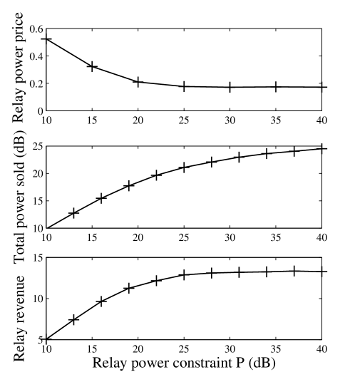
Figure 3: Three-user relay network with Rayleigh fading channels and different relay power constraints.

In the first numerical experiment, the channels are modeled as i.i.d. Rayleigh flat-fading, i.e., $f_{i},h_{i}$, and $g_{i}$ are generated as i.i.d. random variables following the distribution $\mathcal{CN}(0,1)$. We consider a network with three users. The transmit powers of the users are set to be $10$ dB. The simulation results follow the same trend for other values of user powers.

We first investigate the network performance when the relay power ranges from $10$ dB to $40$ dB. This corresponds to the scenario where the total user demand is fixed while the relay power supply increases. We set the relay power price to be the optimal according to Theorem 1. Figure 3 shows the optimal relay power price, the relay power actually sold, and the maximum relay revenue under different relay power constraints. We can see that when the relay has more power to sell, the optimal relay power price is lower, more relay power is sold, and the relay receives more revenue. This complies with one of the laws of supply and demand [33], which says that if supply increases and demand remains unchanged, then it leads to lower equilibrium price and higher quantity.

Figure 4 compares the network sum-rate and fairness of the proposed KSBS-based power allocation with those of the sum-rate-optimal power allocation and the even power allocation. We set the relay power price to be the optimal according to Theorem 1. It can be seen that for the system sum-rate, the difference between our algorithm and the sum-rate-optimal solutions is within $3.5\%$, while it is within $13\%$ between the sum-rate-optimal and the even power solutions. The proposed solution is about $5$ dB superior to the even power allocation. To quantify the fairness of different allocation schemes, we use the average value of the normalized difference: $[\max_{i}(r_{i})-\min_{i}(r_{i})]/\max_{i}(r_{i})$, where $r_{i}$ is the achievable rate of User $i$. A smaller difference indicates a fairer solution. We can see that our solution achieves similar fairness to the even power solution and is fairer than the sum-rate-optimal one.

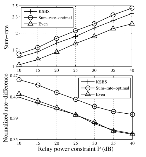
Figure 4: System sum-rate and fairness of a three-user relay network with Rayleigh-fading channels.

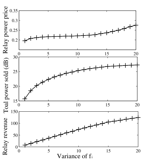
Figure 5: Three-user relay network with Rayleigh fading channels and different variances of $f_{i}$.

Next, we examine the trend of the optimal relay price with an increasing demand. From Lemma 2, $P^{I}_{i}(\lambda)$ is a non-decreasing function of $|f_{i}|^{2}$. So, we can use an increasing $|f_{i}|^{2}$ to simulate the increasing user demand. In this numerical experiment, we again consider a three-user network and model all channels as independent circularly symmetric complex Gaussian random variables with zero-mean, that is, they are independent Rayleigh flat-fading channels. The variances of all $g_{i}$’s and $h_{i}$’s are 1, while the variance of all $f_{i}$’s ranges from 1 to 20. A larger variance means a higher average value of $|f_{i}|^{2}$, which on average means a higher power demand from the users. The transmit power of the users is set to be $10$ dB and relay power is set to be $20$ dB. Figure 5 shows the optimal relay power price, the actual relay power sold, and the maximum relay revenue with different variances of $f_{i}$. We can see that as the variance of $f_{i}$ increases, the optimal relay price increases, more relay power is sold, and the maximum relay revenue increases. This fits one of the laws of supply and demand, which says, if the supply is unchanged and demand increases, it leads to higher equilibrium price and quantity.

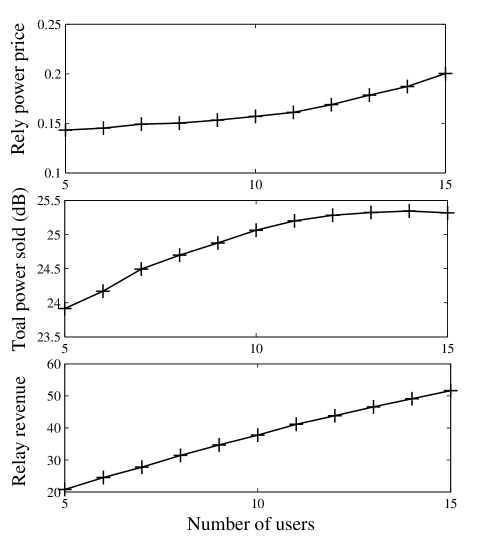
Figure 6: Three-user relay network with Rayleigh fading channels and different numbers of users.

In the third numerical experiment, we examine the relationship between the optimal relay price and the number of users. We assume that the relay power is fixed to be $20$ dB. The user power is fixed as $10$ dB but the number of users vary from $5$ to $15$. All channels are generated following the distribution $\mathcal{CN}(0,1)$. Figure 6 shows the optimal relay power price, the total relay power sold, and the maximum relay revenue with different numbers of users. We can see that as the number of users increases, the optimal relay power price increases, the relay power actually sold increases, and the maximum relay revenue increases. Figure 6 verifies the same law as Figure 5, which says, if the supply is unchanged and demand increases, it leads to higher equilibrium price and quantity.

VI-B Static Network with Path-Loss Channel Only

In this subsection, we study a static network whose channels are deterministic instead of random. The network has three users, one relay, and three destinations. The relative positions of the nodes are shown in Figure 7, where the coordinates of User 1-3, the relay, and Destination 1-3 are (-15, 3), (-10, 0), (-5, -3), (0, 0), and (5, 3), (5, 0), (5, -3), respectively. We consider the path-loss effect of wireless channels only by assuming that the channel gains are inverse proportional to the distance squared. In Figure 7, User 1 is the farthest from its destination and thus has the worst channel; while User 3 is the closest to its destination and has the best channel. The power of the users is set to be $10$ dB and the power of the relay is set to be $15$ dB.

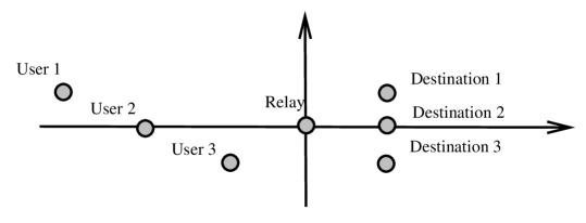
Figure 7: A three-user static network.

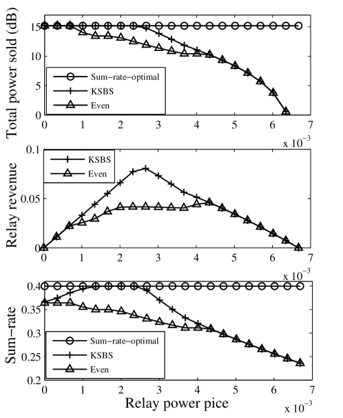
Figure 8: Power allocation, relay revenue, and sum-rate in three-user relay network with static channels.

In Figure 8, the total power sold to the three users, the relay revenue, and the network sum-rate are shown as the relay power price varies. Three power allocation solutions are presented: the proposed KSBS-based power allocation, the sum-rate-optimal power allocation, and the even power allocation. Note that the sum-rate-optimal allocation solution aims to maximize the network sum-rate, is independent of the relay power price, and allocates all the relay power $P$ to the three users. We can observe from Figure 8 that, when the price is higher, with the KSBS-based and the even power allocation schemes, the users purchase less power from the relay and the total power demand is smaller. For example, using the KSBS-based allocation scheme, the total power demand is less than $P$ when the price is higher than $0.0023$. Now let us look at different price ranges separately. First, we can see that in the price range $[0,0.0007]$, both KSBS-based and the even power allocation schemes sell all relay power to the users. This is because in this price range, $P_{i}^{I}(\lambda)\geq P/3$ for $i=1,2,3$, thus with the even power allocation, each user will buy $P/3$, and all relay power will be sold; for the KSBS-based power allocation, $\sum^{3}_{i=1}P_{i}^{I}(\lambda)\geq P$, so all power of the relay will be purchased by the users based on Lemma 4. Second, when $\lambda\geq 0.0047$, the even power and the KSBS-based schemes give the same power allocation results. This is because in this price range, all three users’ ideal power demands are no more than $P/3$, that is, $P_{i}^{I}(\lambda)\leq P/3$ for $i=1,2,3$ and $\sum^{3}_{i=1}P_{i}^{I}(\lambda)\leq P$. In this scenario, from Lemma 4, both the even power allocation and the KSBS-based schemes assign the ideal power demand $P_{i}^{I}(\lambda)$ to User $i$, and the two schemes have the same performance. And when $\lambda$ is in the range $[0.0007,0.0047]$, the KSBS-based power allocation demands more relay power than the even power allocation, and thus the relay receives a higher revenue in this range. This is because with the even power allocation, a user cannot request more than $1/3$ of the total relay power, while the KSBS-based scheme does not have this constraint and thus enables users to request more power. Furthermore, when $\lambda$ is $0.0027$ and the KSBS-based scheme demands $91\%$ of the relay power to be sold to the users, the relay revenue is maximized. At this relay power price, the network sum-rate difference between the proposed KSBS-based solution and the sum-rate-optimal power allocation is only about $2\%$. The sum-rate difference between the even power and the sum-rate-optimal schemes, however, is $23\%$ at the price $\lambda=0.0047$, which is the relay revenue maximizing price under the even power allocation. For any relay price, the sum-rate difference between the even power and the sum-rate-optimal schemes is no less than $9\%$.

TABLE I: Achievable rates, normalized rate-difference, and the system sum-rate in three user relay network with static channels

	Sum-rate	0		0.0013		0.0027		0.0047		0.0053
	-optimal	Even	KSBS	Even	KSBS	Even	KSBS	Even	KSBS	Even	KSBS
$r_{1}$	0.0356	0.0498	0.0499	0.0356	0.0356	0.0356	0.0356	0.0356	0.0356	0.0356	0.0356
$r_{2}$	0.0838	0.1017	0.0994	0.1017	0.0991	0.0823	0.0823	0.0627	0.0627	0.0627	0.0627
$r_{3}$	0.2802	0.2127	0.2169	0.2127	0.2643	0.2127	0.2727	0.1992	0.1992	0.1777	0.1777
Rate-difference	0.8729	0.7658	0.7701	0.8325	0.8652	0.8325	0.8694	0.8211	0.8211	0.7995	0.7995
Sum-rate	0.3997	0.3641	0.3662	0.3500	0.3989	0.3306	0.3907	0.2975	0.2975	0.2760	0.2760

To further compare the performance of the three schemes, Table I shows each user’s achievable rate, the normalized rate-difference, and the network sum-rate with the three power allocation schemes at the relay power prices $0$, $0.0013$, $0.0027$, $0.0047$ and $0.0053$. Recall that a smaller normalized rate-difference represents a fairer power allocation. As can be seen from Table I, the proposed KSBS-based scheme achieves a smaller normalized rate difference than the sum-rate-optimal solution for all relay prices, while the network sum-rate difference between these two schemes is small. It shows that the proposed solution is fairer than the sum-rate-optimal solution with comparable network sum-rate. In sum, Figure 8 and Table I show that for the simulated network, the proposed KSBS-based power allocation and relay pricing solutions achieve close-to-optimal sum-rate, in the mean while, they also maximize the relay revenue and achieve fairness among users.

To compare the sum-rates of the proposed solutions and the sum-rate-optimal solution, we show in Figure 9 the network sum-rate of the proposed relay pricing and power allocation solutions as the relay power constraint $P$ varies. We can see that when the relay power constraint $P$ is small, indicating high demand and low supply, the sum-rate of the proposed solution is almost the same as the optimal sum-rate of the network. As the relay power constraint $P$ increases, indicating low demand and high supply, the sum-rate difference between the proposed solutions and the sum-rate-optimal solution increases. When the relay power is $25$ dB, the difference is about $6\%$. The optimal relay price, on the other hand, decreases as $P$ increases. These verifies the same law of supply and demand with Figure 3, which says, if supply increases and demand remains unchanged, then it leads to lower equilibrium price.

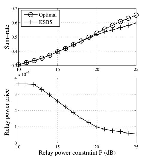
Figure 9: Sum-rate and relay power price in three user relay network with static channels.

VII Conclusion

In this paper, we study the relay power allocation problem in a multi-user single-relay network. By introducing a relay power price, we take into consideration the incentives for cooperation at the relay in helping the users. The Stackelberg game is used to model the interaction between the relay and the users, in which the relay acts as the leader who sets the price of its power to gain the maximum revenue and the users act as followers who pay for the relay service. To model the competition among users, a bargaining game and its KSBS are used for a fair power allocation. We analytically solve the optimal relay price, while the problem of relay power allocation among users is transformed into a convex optimization problem and can be solved with efficient numerical methods. Simulation results show that our solutions reflect the laws of supply and demand, give better user utilities and relay revenue than even power allocation, and approach the sum-rate-optimal power allocation in terms of network sum-rate for a wide range of network scenarios.

References

- [1] A. Nosratinia, T. E. Hunter, and A. Hedayat, “Cooperative communication in wireless networks,” IEEE Communication Magazine, vol. 42, no. 10, pp. 74-80, Oct. 2004.
- [2] A. Gosh and D. R. Wolter, “Broadband wireless access with WiMax/802.16: current performance benchmarks and future potential,” IEEE Communication Magazine, vol. 43, no. 2, pp. 129-136, Feb. 2005.
- [3] L. N. Laneman, D. N. C. Tse, and G. W. Wornell, “Cooperative diversity in wireless networks: efficient protocols and outage behavior,” IEEE Transactions on Information Theory, vol. 50, no. 12, pp. 3062-3080, Dec. 2004.
- [4] R. Annavajjala, P. C. Cosman, and L. B. Milstein, “Statistical channel knowledge-based optimum power allocation for relaying protocols in the high SNR regime,” IEEE Transactions on Selected Areas in Communications, vol. 25, no. 2, pp. 292-305, Feb. 2007.
- [5] S. Serbetli and A. Yener, “Relay assisted F/TDMA ad hoc networks: node classification, power allocation and relaying strategies,” IEEE Transactions on Selected Areas in Communications, vol. 56, no. 6, pp. 937-947, Feb. 2007.
- [6] K. T. Phan, Le-Ngoc Tho, S. A. Vorobyov, and C. Tellambura, “Power allocation in wireless multi-user relay networks,” IEEE Transactions on Wireless Communications, vol. 8, no. 5, pp. 1536-1276, May 2009.
- [7] Y. Jing and H. Jafarkhani, “Network beamforming using relays with perfect channel information,” IEEE Transactions on Information Theory, vol. 55, no. 11, pp. 2499-2517, June 2009.
- [8] K. T. Phan, Le-Ngoc Tho, S. A. Vorobyov, and C. Tellambura, “Distributed power allocation strategies for parallel relay networks,” IEEE Transactions on Wireless Communications, vol. 7, no. 2, pp. 552-561, Feb. 2008.
- [9] J. Cai, X. Shen, J. W. Mark, and A. S. Alfa, “Semi-distributed user relaying algorithm for amplify-and-forward wireless relay networks,” IEEE Transactions on Wireless Communications, vol. 7, no. 4, pp. 1348-1357, Apr. 2008.
- [10] L. Sankaranarayanan, G. Kramer, and N. B. Mandayam, “Hierarchical sensor networks: capacity theorems and cooperative strategies using the multiple-access relay channel model,” in Proc. of First IEEE Conf. Sensor Ad Hoc Commun., Santa Clara, CA, pp. 1-10, 2004.
- [11] L. Sankaranarayanan, G. Kramer, and N. B. Mandayam, “Capacity theorems for the multiple-access relay channel,” in Proc. of 42nd Annual Allerton Conf. Commun. Control Comput., Monticello, IL, pp. 1782-1791, Sep. 2004.
- [12] L. Li, Y. Jing, and H. Jafarkhani, “Multisource transmission for wireless relay networks with linear complexity,” IEEE Transactions on Signal Processing, vol. 59, pp. 2898-2912, June 2011.
- [13] L. Li, Y. Jing, and H. Jafarkhani, “Interference cancellation at the relay for multi-user wireless cooperative networks,” IEEE Transactions on Wireless Communications, vol. 10, no. 3, pp. 930-939, Mar. 2011.
- [14] T. Wang and G. B. Giannakis, “Complex field network coding for multiuser cooperative communications,” IEEE Journal on Selected Areas in Communications, vol. 26, no. 3, pp. 561-571, Apr. 2008.
- [15] S. Yao and M. Skoglund, “Analog network coding mappings in Gaussian multiple-access relay channels,” IEEE Transactions on Communications, vol. 58, no. 7, pp. 1973-1983, July 2010.
- [16] G. A. Sidhu and F. Gao, “Resource allocation for relay aided uplink multiuser OFDMA system,” in Proc. of Wireless Communications and Networking Conference (WCNC), 2010 IEEE, pp. 1-5, Apr. 2010.
- [17] A. MacKenzie and L. DaSilva, Game theory for wireless engineers, Morgan Claypool publishers, 2006.
- [18] W. Saad, Z. Han, M. Debbah, and A. Hjørungnes, “A distributed coalition formation framework for fair user cooperation in wireless networks,” IEEE Transactions on Wireless Communications, vol. 8, no. 9, pp. 4580-4593, Sep. 2009.
- [19] Z. Zhang, J. Shi, H. Chen, M. Guizani, and P. Qiu, “A cooperation strategy based on Nash bargaining solution in cooperative relay networks,” IEEE Transactions on Vehicular Technology, vol. 57, no. 4, pp. 2570-2577, July 2008.
- [20] G. Zhang, H. Zhang, L. Zhao, W. Wang, and L. Cong, “Fair resource sharing for cooperative relay networks using Nash bargaining solutions,” IEEE Communications Letters, vol. 13, no. 6, pp. 381-383, June 2009.
- [21] S. Ren and M. van der Schaar, “Distributed power allocation in multi-user multi-channel cellular relay networks,”IEEE Transactions on Wireless Communications, vol. 9, no. 6, pp. 1952-1964, June 2010.
- [22] N. Shastry and R. S. Adve, “Stimulating cooperative diversity in wireless ad hoc networks through pricing,” in Proc. IEEE Int. Conf. Commun., Jun. 2006.
- [23] O. Ileri, S. C. Mau, and N. B. Mandayam, “Pricing for enabling forwarding in self-configuring ad hoc networks,” IEEE Journal on Selected Areas in Communications, vol. 23, no. 1, pp. 151-162, Jan. 2005.
- [24] B. Wang, Z. Han, and K. J. R. Liu, “Distributed relay selection and power control for multiuser cooperative communication networks using Stackelberg Game,” IEEE Transactions on Mobile Computing, vol. 8, no. 7, pp. 975-990, July 2009.
- [25] S. Ren and M. van der Schaar, “Pricing and distributed power control in wireless relay networks,” IEEE Transactions on Signal Processing, vol. 59, no. 6, pp. 2913-2926, June 2011.
- [26] M. O. Hasna and M. S. Alouini, “End-to-end performance of transmission systems with relays over Rayleigh-fading channels,” IEEE Transactions on Wireless Communications, vol. 2, no. 6, pp. 1126-1131, Nov. 2003.
- [27] M. Hasna and M. S. Alouini, “Harmonic mean and end-to-end performance of transmission systems with relays,” IEEE Transactions on Communications, vol. 52, no. 1, pp. 130-135, Jan. 2004.
- [28] D. Fudenberg and J. Tirole, Game Theory. MIT Press, 1991.
- [29] E. Kalai and M. Smorodinsky, “Other solutions to Nash’s bargaining problem,” Econometrica, vol. 43, pp. 513-518, May 1975.
- [30] S. Boyd and L. Vandenberghe, Convex optimization. Cambridge university Press, 2004.
- [31] A. Muthoo, Bargaining theory with applications. Cambridge university Press, 1999.
- [32] D. P. Palomar and J. R. Fonollosa, “Practical algorithms for a family of waterfilling solutions,” IEEE Transactions on Signal Processing, vol. 53, no. 2, pp. 686-695, Feb. 2005.
- [33] D. Besanko and R. R. Braeutigam Microeconomics. Wiley Press, 2005.