Reliability of NH₃ as the temperature probe of cold cloud cores

Abstract

Context. The temperature is a central parameter affecting the chemical and physical properties of dense cores of interstellar clouds and their potential evolution towards star formation. The chemistry and the dust properties are temperature dependent and, therefore, interpretation of any observation requires the knowledge of the temperature and its variations. Direct measurement of the gas kinetic temperature is possible with molecular line spectroscopy, the ammonia molecule, NH₃, being the most commonly used tracer.

Aims. We want to determine the accuracy of the temperature estimates derived from ammonia spectra. The normal interpretation of NH₃ observations assumes that all the hyperfine line components are tracing the same volume of gas. However, in the case of strong temperature gradients they may be sensitive to different layers and this could cause errors in the optical depth and gas temperature estimates.

Methods. We examine a series of spherically symmetric cloud models, 1.0 and 0.5 $M_{\sun}$ Bonnor-Ebert spheres, with different radial temperature profiles. We calculate synthetic NH₃ spectra and compare the derived column densities and temperatures to the actual values in the models.

Results. For high signal-to-noise observations, the estimated gas kinetic temperatures are within $\sim$0.3 K of the real mass averaged temperature and the column densities are correct to within $\sim$10%. When the S/N ratio of the (2,2) spectrum decreases below 10, the temperature errors are of the order of 1 K but without a significant bias. Only when the density of the models is increased by a factor of a few, the results begin to show significant bias because of the saturation of the (1,1) main group.

Conclusions. The ammonia spectra are found to be a reliable tracer of the real mass averaged gas temperature. Because the radial temperature profiles of the cores are not well constrained, the central temperature could still be different from this value. If the cores are optically very thick, there are no longer guarantees of the accuracy of the estimates.

1 Introduction

The dense molecular cloud cores are of particular interest because their collapse can lead to the formation of new stars. To understand the star formation process, one needs to understand the physical and chemical properties of the cores. The temperature of the cores, especially as a function of position, is difficult to measure and yet it affects everything from core stability to chemistry and dust evolution.

Dust and gas become thermally coupled only at high densities, $n$(H₂)$\sim 10^{5}$ cm^-3 and above (Goldsmith 2001). Because the continuum surface brightness is strongly affected by the warm outer cloud layers, observations of the dust emission are not ideal to determine the gas temperature at the centre of the dense cores. The widths of molecular lines can sometimes be used to derive stringent limits on the gas temperature (e.g., Harju et al. 2008) but the value of this method is limited by the presence of turbulent velocity component.

In observations of most molecules, it is difficult to separate the effects of density, optical depth, and temperature. The situation is different for ammonia, NH₃, whose rotational energy is characterised by the quantum numbers ($J$,$K$). Because the dipole transitions between the different $K$ ladders are forbidden, their relative populations depend only on collisions and thus measure the gas kinetic temperature. Each rotational state ($J$,$K$) is further divided to inversion doublets. The inversion transitions (1,1) and (2,2) are at 23.7 GHz and 23.72 GHz respectively, and are easily observable from the ground. The inversion transitions also have a hyperfine structure. For example the (1,1) spectrum contains 18 components from which at least five separate groups of lines are usually discernible. The intensity ratio of the hyperfine components provides a convenient tool to estimate the line optical depths. Because of these properties, ammonia is a common tool for gas temperature measurements, especially in the case of dense cores (Ho & Townes 1983). The high critical density ($\sim 2\cdot 10^{3}$ cm^-3 for the (1,1) transition as calculated from the ratio of the spontaneous and collisional de-excitation rates at the temperature of 15 K) guarantees that one is measuring temperature of dense gas. On the other hand, NH₃ is resilient against depletion and the abundance is observed to drop only in the very densest and coldest cores (Bergin & Tafalla 2007).

The analysis of NH₃ is based on the assumption that the ($J$,$K$) transitions and their different hyperfine components are all tracing the same physical region. Because of the different optical depths, the weaker hyperfine components could be more sensitive to deeper layers in the cloud. The effect should become noticeable if the main lines are moderately optically thick and the source has strong temperature gradients.

The temperature structure of quiescent cores can, in principle, be calculated from the balance of the various heating and cooling mechanisms (e.g. Goldsmith 2001; Galli et al. 2002). The gas within the cores is heated by the cosmic rays and the external stellar radiation field and it is cooled down by the line radiation from a number of atomic and molecular species. Depending on the temperature difference between the gas and the dust, the gas-dust collisions can result in either heating or cooling of the gas. Juvela & Ysard (2011) discussed the range of possible temperature profiles in dense cores, emphasising the uncertainties associated with many of the contributing factors (e.g., the external radiation field, the gas-dust coupling, and the abundances of the species responsible for the main cooling lines). In this paper we use the models of Juvela & Ysard (2011) to examine the reliability of the ammonia temperature estimates in the presence of radial temperature variations.

The content of the paper is the following. In Sect. 2 we present the methods concerning the core models, the calculation of synthetic ammonia spectra, and the derivation of temperature and column density estimates. The results are presented in Sect. 3, where we compare the derived estimates to the corresponding actual values in the models, in particular studying the effects of observational noise and increased column densities. The final conclusions are presented in Sect. 5.

2 Methods

2.1 Core models

We use the cloud models discussed by Juvela & Ysard (2011). These are 0.5 $M_{\sun}$ and 1.0 $M_{\sun}$ Bonnor-Ebert spheres ($\xi$=6.5, $T_{\rm kin}$=10 K) for which the gas temperatures were calculated under different hypotheses. This resulted in a set of radial temperature profiles with varying shapes, the temperature being of the order of 10 K. While the dust temperature decreases inwards in starless cores, the situation can be different for the gas temperature because of the efficient molecular line cooling in the outer part. In the models, the gas temperature profiles were mostly increasing towards the centre. When the photoelectric heating was included, the situation is reversed and the surface temperature is raised close to 20 K.

The calculations follow Goldsmith (2001) apart from the fact that the cooling rates due to line emission are obtained with a Monte Carlo radiative transfer program. The cooling rates are calculated directly for ¹²CO, ¹³CO, C¹⁸O, C, CS, and o-H₂O. The rates of the last two species are multiplied by 10.0 and 2.0, respectively, to take into account the contribution of other species. We examine the following cases without the photoelectric heating: the default model (‘def’), the low abundance model ($\chi$), the weak gas-dust coupling model ($\Lambda_{\rm gd}$), the small velocity dispersion model ($\sigma_{\rm v}$), and the large velocity gradient model ($v$). The names refer to the temperature calculations in Juvela & Ysard (2011).

The $def$-model was obtained assuming $\sigma_{\rm v}$=1.0 km s^-1 line widths (Doppler width) and constant abundances in the calculation of the cooling lines, no large scale velocity field, and a coupling between the gas and dust temperatures that followed that presented in Goldsmith (2001). In the $\sigma_{\rm v}$-model, the turbulent linewidth changes as a step function from 1.0 km s^-1 in the outer part, outside the half radius, to 0.1 km s^-1 within the inner core. The $v$-model is the only one with a large scale velocity field. It has radial infall velocities that increase linearly from 0 km s^-1 at the surface to 1.0 km s^-1 in the centre. The name of the low abundance model ($\chi$) refers to the calculations of the gas kinetic temperature where the abundance of the cooling species was assumed to be lower at the centre of the core. This was implemented as a step function with a factor of ten difference between the inner and outer parts. However, in the modelling of the NH₃ spectra, the fractional abundance of para-NH₃ is always kept at a constant value of 10^-8 (e.g. Hotzel et al. 2001; Tafalla et al. 2004). This applies also to the $\chi$-model. The photoelectric heating is included only in one model (model $PEH$) where the model cloud is assumed to be illuminated by an unattenuated interstellar radiation field (Mathis et al. 1983). For the details of the calculations of the $T_{\rm kin}$ profiles, see Juvela & Ysard (2011).

In addition to the above described models, we consider cases where the kinetic temperatures are the same but the turbulent line width is decreased by a factor of ten in the NH₃ calculations. In particular, in the central part of the $\sigma_{\rm V}$-model the linewidth then becomes practically thermal. We use the Juvela & Ysard (2011) results only as examples of the possible shapes of the temperature profiles and the purpose of the present paper is to probe their effect on the analysis of ammonia spectra at a general level.

Table 1: The main core models.

Model	Modification	$T_{\rm kin}$ ranges of the 0.5
		and 1.0 M☉ models (K)
Default	–	5.3-9.3, 4.6-8.4
$\chi$	$\chi=(0.1-1.0)$  $\chi^{\rm default}$	5.3-11.0, 4.8-11.0
$\Lambda_{\rm g,d}$	$\Lambda_{\rm g,d}$=(0.3-1.0)  $\Lambda_{\rm g,d}^{\rm default}$	6.4-10.0, 5.3-8.5
$\sigma_{\rm v}$	$\sigma_{\rm v}$=(0.1-1.0)  $\sigma_{\rm v}^{\rm default}$	5.3-10.9, 4.8-11.4
$v_{\rm radial}$	0-1.0 km s-1	5.3-9.1, 4.8-8.3
PEH	include $\Gamma(PEH)$ for	9.2-14.7, 9.2-19.1
	$\zeta$=3$\cdot 10^{17}$ s-1

2.2 Synthetic spectra

For each model, synthetic para-NH₃ (1,1) and (2,2) spectra were obtained with the help of radiative transfer calculations. The non-LTE radiative transfer problem is solved with a Monte Carlo program (Juvela 1997). The the model clouds are divided into 100 shells. To get better resolution in the outer regions where the excitation conditions can change more rapidly, the thickness of the shells was decreased towards the surface. The radius of the innermost sphere and the thickness of the outermost shell are, respectively, $\sim$6% and 0.7% of the radius of the model cloud.

The ammonia spectra are calculated following the prescription presented in Keto et al. (2004). The non-LTE populations of the ($J$,$K$) states of para-NH₃ are obtained from the radiative transfer calculations where, within each state, an LTE distribution is assumed between the hyperfine levels (i.e., distribution according to the statistical weights of the transitions). In the radiative transfer calculations, we take into account the hyperfine components of the (1,1) and (2,2) lines. These consist of 18 and 21 components, respectively. In the final synthetic (1,1) and (2,2) spectra, many of these components are blended together. The molecular parameters for the ($J$,$K$) lines are from the Lamda database (Schöier et al. 2005) and the frequencies and relative intensities of the hyperfine lines were taken from Kukolich (1967).

The synthetic spectra are calculated for a pencil beam (i.e., for a single line-of-sight through the centre of the core) and averaged over a Gaussian beam with the FWHM equal to the core radius. Because the excitation of the molecules varies along the line of sight and the hyperfine components have different optical depths, the observed intensity ratios between hyperfine components can vary depending on the optical depth and temperature structure of the model. Figure 1 shows examples of the simulated spectra.

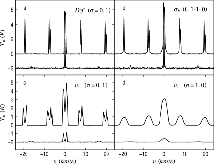
Figure 1: Examples of simulated ammonia spectra. Each frame shows the (1,1) (the upper line) and the (2,2) spectral profiles. For the plotting, the latter have been scaled by a factor of 3 and shifted by -2 K. The text in the upper right hand corner indicates the model in question and, in parentheses, the turbulent line width used in the calculation of the NH₃ spectra.

2.3 Analysis of the spectra

To derive estimates of the column densities and gas kinetic temperatures, we subject the synthetic NH${}_{3}(1,1)$ and NH${}_{3}(2,2)$ spectra to standard analysis as described in Ho & Townes (1983), Walmsley & Ungerechts (1983), and Ungerechts et al. (1986). The hyperfine structure of the NH${}_{3}(1,1)$ line is fitted using a $\chi^{2}$ routine assuming a gaussian velocity distribution and that the different hyperfine states are populated according to LTE. The fit results are used to calculate the optical thickness profile $\tau(v)$. The peak value $\tau_{\rm peak}$, and the brightness temperature in the corresponding channel (usually coincident with the intensity maximum $T_{\rm B,peak}$) are substituted in the antenna equation to derive the excitation temperature, $T_{\rm ex}$, of the transition. The integrated optical thickness, $\int\tau(v)dv$, where $v$ is the radial velocity, and $T_{\rm ex}$ give the column density in the upper transition level, $N_{\rm u}(1,1)$, from the formula

$$N_{\rm u}(1,1)\;=\;\frac{8\pi}{\lambda_{11}^{3}}\;\frac{1}{A_{\rm ul}}\;F(T_{11},T_{\rm ex})\;\int\,\tau(v)\,dv\;,$$

where $A_{\rm ul}$ is the Einstein coefficient for spontaneous emission, $\lambda_{11}=c/\nu_{11}$ is the wavelength of the transition, $T_{11}=h\nu_{11}/k_{\rm B}$, and the function $F(T_{0},T)$ is defined by

$$F(T_{0},T)\equiv\frac{1}{e^{T_{0}/T}-1}\;.$$

Adding together the upper and lower levels of the inversion transition, the total column density of ammonia in the (1,1) level is

$$N(1,1)\;=\;N_{\rm u}\;(1+e^{T_{11}/T_{\rm ex}})\,.$$

The column density of the (2,2) level, $N(2,2)$, can be derived using two slightly different methods: a) by estimating $\tau$ and $T_{\rm ex}$ from the hyperfine fit as in the case of (1,1); or b) by assuming that $T_{\rm ex}$ is the same as for the $(1,1)$ transition and that the (2,2) line is optically thin. In the case b the integral $\int\tau(v)dv$ is estimated from the integrated intensity of the (2,2) main group using the antenna equation. Usually only the method b is feasible for observational data of cold clouds because the (2,2) satellites are very weak and buried in the noise. In the present paper we use the method b to do the analysis.

The rotational temperature, $T_{12}$, is defined with the Boltzmann equation

$$\frac{N(2,2)}{N(1,1)}=\frac{5}{3}e^{-41.5/T_{12}}\;.$$

The kinetic temperature, $T_{\rm kin}$, is estimated using the three level approximation (including the levels $(J,K)$=(1,1), (2,1) and (2,2)) as outlined by Walmsley & Ungerechts (1983). The temperature dependence of the ratio of the collisional coefficients $C_{22\rightarrow 21}/C_{22\rightarrow 11}$ was estimated adopting the coefficients of Danby et al. (1988). The method is the same as used in Harju et al. (1993). The resulting relationship between $T_{12}$ and $T_{\rm kin}$ is very close to that given in the Appendix B of Tafalla et al. (2004). In cold gas, the sum of the column densities of the (1,1) and (2,2) levels is almost equal to the total column density of para-NH₃ as the populations of the higher rotational levels are negligible. We calculate these column density estimates from the synthetic observations and compare with the corresponding true values in the model clouds.

3 Results

3.1 The basic models

The derived para-NH₃ column densities and the gas kinetic temperatures were compared to the corresponding true values that were calculated as the mass averaged quantities in the model clouds, averaged over the same beam as what was used in the calculation of the synthetic ammonia spectra.

The main results are presented in Figs. 2– 4. The profiles of the kinetic temperature $T_{\rm kin}$ are shown as solid black curves. These are a critical input parameter for the simulation of the ammonia spectra. Without the photoelectric heating, $T_{\rm kin}$ increases towards the cloud centre. The central temperature is further increased when, within one half of the cloud radius, the abundance of the cooling species is decreased (model $\chi$) or the turbulent linewidth is decreased. In model $\Lambda_{\rm g,d}$, the gas-dust coupling is weakened in the inner core, leading to a small decrease in the temperature because $T_{\rm dust}>T_{\rm gas}$. We do not claim that all these temperature profiles are likely to be found in starless cores. However, for the present case the most important fact is that they probe a wide range of $T_{\rm kin}$ profiles that potentially could result in a bias in the $T_{\rm kin}$ estimates.

Figure 2 shows the $T_{\rm kin}$ estimates for the 1 $M_{\sun}$ cloud. The horizontal thin and thick lines indicate the true mass averaged temperatures for a single line-of-sight through the centre of the model cloud (thin line) or weighted with a gaussian beam with a FWHM equal to cloud radius. The dashed lines are correspondingly the $T_{\rm kin}$ estimates derived from the NH₃ spectra observed with a pencil beam or the larger gaussian beam. In the frames also are given the true and estimated column densities. For comparison, Figs. 3 and  4 show the results for 0.5 $M_{\sun}$ models and for 1 $M_{\sun}$ models with a smaller turbulent linewidth ($\sigma\leq$0.1 km s^-1).

The temperature estimates derived from the simulated NH₃ spectra are correct to within 0.5 K and the errors of the column density values are $\sim$10% or less. This applies to the observations conducted with a pencil beam and most observations with a gaussian beam. When one includes the convolution with the large beam, the temperature values reflect more the values found in the outer part of the cloud. However, compared to the beam averaged real kinetic temperature, the values appear to be biased towards the $T_{\rm kin}$ in the cloud centre. The error is largest for the $\sigma_{\rm v}$ model where it can approach 1 K (Fig. 2).

The spectra of the $v$-model are double peaked because of the infall motion that at the centre leads to maximum line-of-sight velocities of $\pm$1 km s^-1 (see Fig. 1). The redshifted peak is stronger than the blueshifted peak. This is opposite to the expected behaviour in contracting clouds and is caused by the fact that the temperature is decreasing towards the core centre within the innermost $\sim$20% of the cloud radius. When the spectra are modelled as the sum of two components, the individual features described with gaussians, the analysis recovers the correct solution with good accuracy. In the case of narrow lines ($\sigma\leq$0.1 km s^-1) a single component fit to the two velocity components would result in an error of $\sim$1 K. On the other hand, when that model is observed with a larger beam, only a single velocity component remains visible. In Fig. 4 the beam convolved data were fitted with a single gaussian and the pencil beam observations with two components. In both cases the temperature estimates remain within $\sim$0.2 K of the correct value.

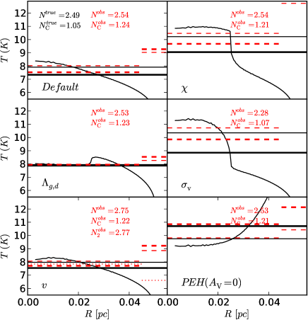
Figure 2: The radial temperature profiles (solid black curves), the estimated temperatures (dashed red lines), and the mass averaged true temperatures (black horizontal lines) for the one solar mass models. The thin lines correspond to the data on a single line-of-sight through the cloud centre and the thick lines to data averaged with a gaussian beam. In the right hand part of each frame, the difference between the estimated and the real mass averaged $T_{\rm kin}$ has been scaled by a factor of ten for better visibility. The column densities derived from the observations are indicated in each frame (units of $10^{14}$ cm^-2), the subscript $C$ denoting the case with beam convolution. The true column densities are given in the first frame. For the $v$-model, the dotted line and the lower text entry indicate the result from a fit with two velocity components (pencil beam only).

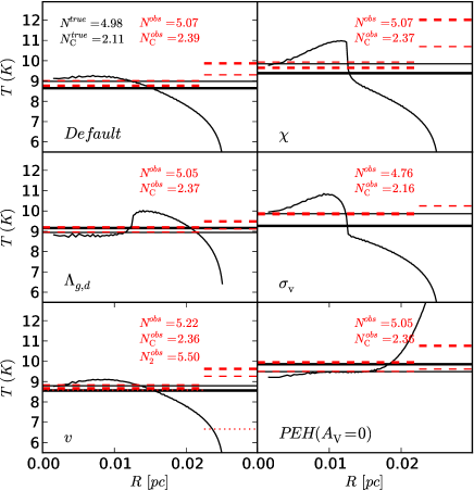
Figure 3: As Fig. 2 but for the half solar mass core.

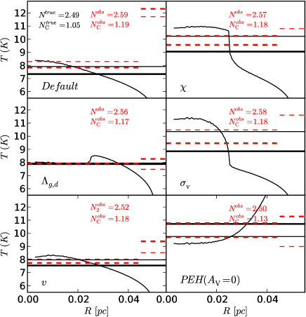
Figure 4: As Fig. 2 but with the synthetic ammonia spectra modelled with a smaller, 0.1 km s^-1 turbulent linewidth. For the model $v$, the pencil beam observations are fitted with two velocity components and the convolved spectra with a single velocity component.

3.2 The influence of noise

The influence of observational noise was examined by analysing a series of spectra with progressively higher signal-to-noise ratios. The S/N ratio is defined as the ratio between the peak intensity of the (2,2) spectrum and the rms noise per channel. The rms noise added to the (1,1) spectra was the same in brightness temperature units. In addition to the default model (marked ‘$def$’), the models with the temperature distributions corresponding to the ‘$\sigma_{\rm v}$’ and ‘$PEH$’ cases were examined, i.e., models with strong inward and outward temperature gradients. Both the $M=0.5\,M_{\sun}$ and $M=1.0\,M_{\sun}$ cloud models were used, calculating the ammonia spectra with either 1.0 km s^-1 or 0.1 km s^-1 linewidths. Again, the narrower line width is not consistent with the original derivation of the temperature profiles (Juvela & Ysard 2011) but gives some insight to clouds with higher line optical depths.

Figure 5 shows the estimated kinetic temperatures and column densities in relation to their true values in the model clouds. The spectra were calculated using a pencil beam. The S/N covers a range from $\sim$3 to 300 in multiplicative steps of 1.5. For each S/N ratio we show the results from five realizations of spectra, the dashed lines corresponding to their mean value. The results from the $M=0.5\,M_{\sun}$ and the $\sigma_{\rm V}$=0.1 km s^-1 were qualitatively similar.

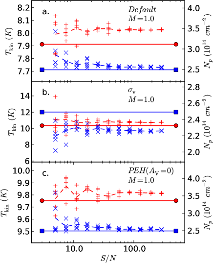
Figure 5: The gas kinetic temperature (plus symbols) and the column density (crosses) estimated from spectra with different signal-to-noise ratios. For each S/N ratio, the figure shows results from five realisations and their average as the dashed lines. The horizontal lines indicate the true values in the models. The three frames correspond to the default model ($def$’), the $\sigma_{\rm V}$-model, and the $PEH$ model, respectively, of the 1.0 $M_{\rm sun}$ cloud.

3.3 Models of high optical depth

In the default 1 $M_{\rm sun}$ model the peak optical depths are $\tau_{\rm(1,1)}$=0.7 and $\tau_{\rm(2,2)}$=0.013. In the 0.5 $M_{\rm sun}$ cloud these increase to 1.2 and 0.04, respectively. When the turbulent linewidth was decreased from 1.0 km s^-1 to 0.1 km s^-1, the values were naturally higher, 4.3 and 0.33 for the (1,1) and (2,2) lines, respectively. However, as the satellite lines continue to be mostly optically thin, this is not a big problem for the analysis of the spectra.

To determine when and how the errors increase to significant levels, we took the 1.0 $M_{\rm sun}$ clouds and calculated a series of models where the densities were multiplied with constant factors $k_{\rm n}$ between 1 and 64. The temperature profiles are taken from the original $\sigma_{\rm v}$ and $PEH$ models (Fig. 2) and are not changed Therefore, the changes will be only because of the increase of the density and the column density. Figure 6 shows the resulting $T_{\rm kin}$ and $N$(para-NH₃) estimates resulting from observations with a pencil beam towards the cloud centre. As expected, the estimates show some bias when the column densities are much higher than for the original 1 M_☉ Bonnor-Ebert spheres. In the $PEH$ model the $T_{\rm kin}$ estimates continue to be very accurate and even in column density the error rises to $\sim 50$% only when the density is some 50 times the original values. In this model, the real temperature is quite constant within the central regions and apparently the optical depths are still not high enough so that the spectra would react to the warm but low density surface layers. The changes were more dramatic in the $\sigma_{\rm v}$-model where the results were essentially wrong after $k_{\rm n}\sim$4. In this model the optical depths were higher to start with, because of the narrow linewidth at the centre.

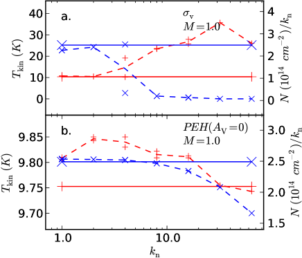
Figure 6: The gas kinetic temperature (plus symbols) and the column density (crosses) when the densities of the 1.0 $M_{\rm sun}$ model are scaled with factors $k_{\rm n}$ in the range of 1-64. The column densities have been normalized with $k_{\rm n}$. The solid lines indicate the true values and the dashed lines are the values deduced from the synthetic observations. The frames correspond to different temperature distributions as marked in the upper right hand corner of each frame.

Figure 7 shows the actual spectra calculated for $k_{\rm n}$=1 and $k_{\rm n}$=32. In the $\sigma_{\rm v}$-model, the main group becomes strongly self-absorbed and, because the kinetic temperature is higher in the centre than at the surface, the intensity of the satellite lines is higher than for the main group. This is, of course, a situation that cannot be accounted for in the analysis assuming a homogeneous medium.

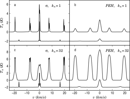
Figure 7: Comparison of the original spectra from the one solar mass $\sigma_{\rm v}$ and the $PEH$ models and the spectra obtained after the densities have been scaled by a factor of $k_{\rm n}$=32. For the plotting, the (2,2) spectra have been scaled by a factor of 3 (upper frames) or 0.5 (lower frames) and shifted by -2 K.

4 Discussion

Tafalla et al. (2004) examined the validity of the kinetic temperature estimates from NH₃ using isothermal models. In the present study, we calculate the mass averaged kinetic temperatures in model clouds with realistic temperature profiles. The values are compared to the kinetic temperature estimates derived with a standard LTE method, using the ammonia spectra ‘observed’ from these models.

The estimated kinetic temperatures were generally found to be very accurate. In the case of model clouds with masses 0.5 $M_{\sun}$ and 1 $M_{\sun}$, the difference between the temperature derived from the NH₃ spectra and the real mass-averaged temperature was of the order of 0.1 K, only rarely approaching 1 K. Similarly, the estimated column densities of para-NH₃ remained correct to within $\sim$10%.

In one of the models the infall velocity produced two velocity components whose presence, in the case of large turbulent linewidths $\sigma_{\rm V}=1.0$ km ^-1, was not immediately obvious from the line profiles. The analysis completed using a single gaussian component still led to only $\sim$1 K error. A fit with two velocity components resulted in twice as high errors in both the temperature and the estimated column density (Fig. 2). When the turbulent line width was reduced in the cloud core so that the velocity components became clearly visible in the (1,1) profiles, the error of a single component fit increased to $\sim$1.5 K and the column density was overestimated by 20% (Fig. 4). However, this time the two component fit did recover the correct results with less than 10% errors. This increases the general confidence in the results of obtained from ammonia spectra observed with adequate resolution. It appears unlikely that the effect of hidden features, e.g. of multiple velocity components, would be amplified in the $T_{\rm kin}$ and $N$ estimates.

When the signal-to-noise of the (2,2) spectra is decreased below S/N$\sim$10, the temperature errors increased in our tests to $\sim$1 K. The results were not significantly biased so that even for a set of sources observed at low S/N, the mean properties should be relatively trustworthy. The sensitivity to noise naturally depends on the width of the lines.

When the column density is increased much beyond that found in our basic models, the (1,1) becomes optically thick and there are no longer guarantees of the accuracy of the results. In particular, the lines might no longer probe the conditions at the centre of very dense cores. We carried out one test with an ad hoc scaling of the densities. The behaviour was found to depend very much on the line widths (affecting the initial line opacity) and the temperature structure of the cloud. In the case with a small turbulent linewidth, $\sigma_{\rm V}=0.1$ km^-1 s^-1, completely wrong results were already encountered with densities a few times higher that those of an 1 $M_{\rm sun}$ Bonnor-Ebert sphere. If the fractional abundance were larger than the 10^-8 assumed in our models, observations of normal hydrostatic cores could be affected. However, in starless cores the values are not likely to be much higher (Hotzel et al. 2001; Tafalla et al. 2002; Crapsi et al. 2007).

Tafalla et al. (2004) found that the excitation temperatures of the (1,1) and (2,2) lines varied by a factor of several. This variation depends on several factors, the cloud optical depth, the volume density, and the variation of the kinetic temperature. Figure 8 shows the situation in those of our 1.0 $M_{\sun}$ models where the difference in the radial kinetic temperature profiles is the largest. In the $\sigma_{\rm V}$ model the kinetic temperature increases inwards and, in combination of higher volume density and enhanced photon trapping, the excitation temperatures at the cloud centre are three times as high as at the cloud boundary. Towards the centre also the difference between the excitation temperatures of the (1,1) and (2,2) transitions becomes more noticeable. On the other hand, in the $PEH$ case the outward increasing kinetic temperature helps to keep the excitation conditions almost constant. Therefore, it is not surprising that the kinetic temperature estimated from the observed spectra remained accurate even when the density was increased (Fig. 6).

Ammonia was found to be a very reliable tracer of the real mass averaged gas temperature within the modelled Bonnor-Ebert spheres. The temperature at the centre of a cloud could still differ from this number by several degrees. In our models this difference was at most $\sim$1 K. However, if the signal from very centre becomes weaker because of a lower abundance combined with a low kinetic and excitation temperatures, the difference can be more significant.

In this paper we have assumed the ammonia abundance to be constant as a function of the cloud radius (see e.g. Tafalla et al. 2006). If the abundance varies, NH₃ is likely to provide accurate estimates of the average temperature weighted not only by the mass but also by the fractional abundance. If the ammonia abundance increases towards the centre (e.g. Tafalla et al. 2002) the result will be a better estimate of the central core temperature. In cores denser than considered here the situation may be reversed as even NH₃ becomes depleted in the very centre of the core (Aikawa et al. 2005). As an illustration of the associated uncertainties, we considered the $\sigma_{\rm v}$ model with 1.0 M_☉, varying the abundance between 10^-7.5 and 10^-8.5 as a linear function of the logarithm of the radius. One obtains an estimate of $T_{\rm kin}$=10.49 K when the abundance increases inwards and 10.59 K when the abundance increases outwards. Both are within 0.25 K of the value from the previous constant abundance model. Thus, in this case the effect of the abundance gradients is not very significant. However, we will return to this questions in future papers that discuss self-consistent models of the chemistry and of the thermal balance.

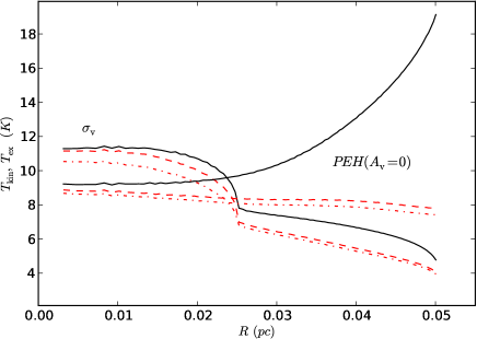
Figure 8: Comparison of temperatures in the $1.0\,M_{\sun}$ cloud models $\sigma_{\rm v}$ and $peh$. Shown are the radial profiles of the kinetic temperature (solid lines) and the excitation temperatures of the (1,1) (dashed line) and (2,2) (dash-dotted line).

5 Conclusions

We have calculated ammonia emission spectra using non-LTE radiative transfer modelling and cloud core temperature profiles taken from the literature. We have carried out analysis of the simulated spectra and compared the results with the true parameters of the model clouds. This has led to the following conclusions:

• For the $\sim$1 $M_{\sun}$ hydrostatic clouds, the kinetic temperatures and column densities derived from the ammonia observations are accurate to better than 10% accuracy.

• The presence of several velocity components can be identified from the line profiles before they have a significant effect on the accuracy of the analysis.

• The uncertainty of the kinetic temperature estimates increases to $\sim$1 K when the signal-to-noise of the (2,2) spectra is decreased to S/N$\sim$10.

• In models of higher density, the behaviour depends the kinetic temperature profile of the cloud. Quite wrong results can already be encountered with models a few times more opaque than the 1 $M_{\rm sun}$ Bonnor-Ebert spheres.

• Apart from the most opaque cores, the ammonia was found to be a very reliable tracer of the mass averaged kinetic temperature. The temperature at the centre of dense cores could still differ from this value by several degrees.