Black Hole Evaporation in a Noncommutative Charged Vaidya Model

Abstract

The aim of this paper is to study the black hole evaporation and Hawking radiation for a noncommutative charged Vaidya black hole. For this purpose, we determine spherically symmetric charged Vaidya model and then formulate a noncommutative Reissner-Nordstr$\ddot{o}$m-like solution of this model which leads to an exact $(t-r)$ dependent metric. The behavior of temporal component of this metric and the corresponding Hawking temperature is investigated. The results are shown in the form of graphs. Further, we examine the tunneling process of the charged massive particles through the quantum horizon. It is found that the tunneling amplitude is modified due to noncommutativity. Also, it turns out that black hole evaporates completely in the limits of large time and horizon radius. The effect of charge is to reduce the temperature from maximum value to zero. It is mentioned here that the final stage of black hole evaporation turns out to be a naked singularity.

Keywords: Noncommutativity; Reissner-Nordstr$\ddot{o}$m-like Vaidya spacetime; Black hole evaporation; Quantum tunneling.
PACS: 04.70.Dy; 04.70.Bw; 11.25.-w

1 Introduction

Classically, the concept of smooth spacetime manifold breaks down at short distances. Noncommutative (NC) geometry gives an impressive structure to investigate short distance spacetime dynamics. In this structure, there exists a universal minimal length scale, $\sqrt{\sigma}$ (equivalent to Planck length). In General Relativity (GR), the effects of NC can be taken into account by keeping the standard form of the Einstein tensor and using the altered form of the energy-momentum tensor in the field equations. This involves distribution of point-like structures in favor of smeared objects . Noncommutative black holes (BHs) require an appropriate framework in which the NC corresponds to GR.

Black hole evaporation leads to comprehensive and straightforward predictions for the distribution of emitted particles. However, its final phase is unsatisfactory and cannot be resolved due to semi-classical representation of Hawking process. Black Hole evaporation can be explored in curved spacetime by quantum field theory but BH itself is described by a classical background geometry. On the other hand, the final stage of BH decay requires quantum gravity corrections while the semi-classical model is incapable to discuss evaporation. Noncommutative quantum field theory (based on the coordinate coherent states) treats short-distance behavior of point-like structures, where mass and charge are distributed throughout a region of size $\sqrt{\sigma}$.

Hawking [1] suggested that a radiation spectrum of an evaporating BH is just like a black body with a purely thermal spectrum, i.e., BH can radiate thermally. Consequently, a misconception [2] was developed with respect to information loss from BH leading to non-unitary of quantum evolution . Accordingly, when a BH evaporates completely, all the information related to matter, falling inside the BH, will be lost. Gibbons and Hawking [3] proposed a formulation to visualize radiation as tunneling of charged particles. In this formulation, radiation corresponds to electron-positron pair creation in a constant electric field whereas the energy of a particle changes sign as it crosses the horizon. The total energy of a pair, created just inside or outside the horizon, would be zero when one member of the pair tunneled to opposite side. Parikh and Wilczek [4] derived Hawking radiation as a tunneling through the quantum horizon on the basis of null geodesics. In this framework, the corrected BH radiation spectrum is obtained due to back-reaction effects. This tunneling process shows that the extended radiation spectrum is not exactly thermal yielding a unitary quantum evolution.

There are two different semiclassical tunneling methods to calculate the tunneling amplitude which leads to the Hawking temperature. The first method, called the null geodesic method, gives the same temperature as the Hawking temperature. The second one named as canonically invariant tunneling, leads to canonically invariant tunneling amplitude and hence the corresponding temperature which is higher than the Hawking temperature by a factor of 2 [5]. Akhmedova et al [6] argued that a particular coordinate transformation resolves this problem in quasiclassical picture.

Alexeyev et al [7] discussed BH evaporation spectra in Einstein-dilaton-Gauss-Bonnet four dimensional string gravity model by using the radial null geodesic method. They showed that BHs should not disappear and become relics at the end of the evaporation process. They investigated numerically the possibility of experimental detection of such remnant BHs and discussed mass loss rate in analytic form. These primordial BH relics could form a part of the non-baryonic dark matter in our universe.

Smailagic and Spallucci [8] found various NC models in terms of coordinate coherent states which satisfy Lorentz invariance, unitarity and UV finiteness of quantum field theory. Nicolini et al. [9] derived the generalized NC metric which does not allow BH to decay lower than a minimal nonzero mass $M_{0}$, i.e., BH remnant mass. The effects of NC BHs have been studied [10, 11] and found consistent results. The evaporation process stops when a BH approaches to a Planck size remnant with zero temperature. Also, it does not diverge rather reaches to a maximum value before shrinking to an absolute zero temperature which is an intrinsic property of manifold. Some other people [12] also explored information loss problem during BH evaporation.

Sharif and Javed [13] investigated quantum corrections of the thermodynamical quantities for a Bardeen charged regular BH by using quantum tunneling approach over semiclassical approximations. In a recent work [14], they have also discussed the behavior of NC on the thermodynamics of this BH. Mehdipour [15] analyzed the tunneling of massive particles through quantum horizon of the NC Schwarzschild BH and derived the modified Hawking radiation, thermodynamical quantities and emission rate. He also discussed stable BH remnant and information loss issues. Nozari and Mehdipour [16] studied the effects of smeared mass and showed that information might be saved by a stable BH remnant during the evaporation process. Mehdipour [17] extended this work for NC Reissner-Nordstr$\ddot{o}$m (RN) BH and determined the emission rate consistent with unitary theory. The same author [18] also formulated a NC Schwarzschild-like metric for a Vaidya solution and analyzed three possible causal structures of BH initial and remnant mass. Also, he studied the tunneling of charged particles across the quantum horizon of the Schwarzschild-like Vaidya BH and evaluated the corresponding entropy.

The purpose of this paper is two fold: Firstly, we formulate NC RN-like solution of the spherically symmetric charged Vaidya model. Secondly, we investigate some of its features. In particular, we explore BH evaporation and Parikh-Wilczek tunneling process. Its format is as follows. In section 2, we solve the coupled field equations for spherically symmetric charged Vaidya model. The effect of NC form of this model is investigated in the framework of coordinate coherent states in section 3. Here, an exact $(t-r)$ dependent RN-like BH solution is obtained. Section 4 yields the behavior of the temporal component of this solution and also provides discussion about BH evaporation in the limits of large time and charge. In section 5, we study Parikh-Wilczek tunneling for such a Vaidya solution and also Hawking temperature in the presence of charge. The tunneling amplitude at which massless particles tunnel across the event horizon is computed. Finally, the conclusion of the work is given in the last section. It is mentioned here that throughout the paper we assume $\hbar=c=G=1$.

2 Charged Vaidya Model

This section is devoted to formulate spherically symmetric charged Vaidya model in the RN-like form by using the procedure given by Farley and D’Eath [19]. Here we shall skip the details of the procedure as it is already available and use only the required results. The spherically symmetric Vaidya form metric is given by (2.34) of [19]

$$ds^{2}=-e^{\nu(t,r)}dt^{2}+e^{\mu(t,r)}dr^{2}+r^{2}d\Omega^{2},$$ (1)

where

$$e^{\nu(t,r)}=\left(\frac{\dot{M}}{\chi(M)}\right)^{2}e^{-\mu},\quad e^{-\mu(t,r)}=1-\frac{2M}{r},\quad d\Omega^{2}=d\theta^{2}+\sin^{2}\theta d\phi^{2},$$

$M(t,r)$ is a slowly-varying mass function and $\chi(M)$ depends on the details of the radiation. The corresponding field equations are [19]

$$\mu^{\prime}=8\pi rT_{rr}+\frac{1-e^{\mu}}{r},$$ (2)

$$\nu^{\prime}=8\pi re^{\mu-\nu}T_{tt}-\frac{1-e^{\mu}}{r},$$ (3)

$$\dot{\mu}=8\pi rT_{tr},$$ (4)

$$1-e^{-\mu}+\frac{1}{2}re^{-\mu}(\mu^{\prime}-\nu^{\prime})-\frac{1}{2}r^{2}R^{(0)}=8\pi T_{\theta\theta}=\frac{8\pi T_{\phi\phi}}{\sin^{2}\theta},$$ (5)

where

$$R^{(0)}=-8\pi{T^{a}}_{a}=-\frac{2}{r^{2}}(1-e^{-\mu})+e^{-\frac{1}{2}(\mu+\nu)}[{(\dot{\mu}e^{\frac{1}{2}(\mu-\nu)})}^{\cdot}-{(\nu^{\prime}e^{\frac{1}{2}(\nu-\mu)})}^{\prime}].$$ (6)

Here dot and prime mean derivatives with respect to time and $r$ respectively. It is mentioned here that Eqs.(2) and (4) represent the Hamiltonian and momentum constraints respectively [20]. Equations (2) and (3) lead to

$$\frac{1}{2}(\mu^{\prime}-\nu^{\prime})=\frac{1-e^{\mu}}{r}$$ (7)

while Eqs.(5) and (6) yield

$$T_{rr}=e^{(\mu-\nu)}T_{tt}.$$ (8)

For the spherically symmetric Vaidya metric of the form (1), we define $e^{-\mu(t,r)}$ by adding charge $Q(t,r)$ as follows

$$e^{-\mu(t,r)}=1-\frac{2M(t,r)}{r}+\frac{Q^{2}(t,r)}{r^{2}}.$$ (9)

Using the procedure [19], one can write from the field equations

$${T^{t}}_{r}e^{\frac{1}{2}(\nu-\mu)}+{T^{t}}_{t}=0.$$ (10)

Also, using Eqs.(2), (4), (8) and (10), we obtain

$$\mu^{\prime}+\frac{e^{\mu}-1}{r}+\dot{\mu}e^{\frac{(\mu-\nu)}{2}}=0.$$ (11)

Inserting the value of $e^{\mu}$ from Eq.(9), it follows that

$$e^{\nu(t,r)}=\left(\frac{\frac{2Q\dot{Q}}{r}-2\dot{M}}{2M^{\prime}-\frac{2QQ^{\prime}}{r}+\frac{Q^{2}}{r^{2}}}\right)^{2}\left(1-\frac{2M}{r}+\frac{Q^{2}}{r^{2}}\right)^{-1}.$$ (12)

The corresponding form of the Vaidya solution [21] will become

$$ds^{2} = -\left(\frac{\frac{2Q\dot{Q}}{r}-2\dot{M}}{2M^{\prime}-\frac{2QQ^{\prime}}{r}+\frac{Q^{2}}{r^{2}}}\right)^{2}\left(1-\frac{2M}{r}+\frac{Q^{2}}{r^{2}}\right)^{-1}dt^{2}$$ (13)

$$+ \left(1-\frac{2M}{r}+\frac{Q^{2}}{r^{2}}\right)^{-1}dr^{2}+r^{2}d\Omega^{2}.$$

This is the spherically symmetric charged Vaidya model.

Now we transform this metric so that it is in RN-like form. For this purpose, we write Eq.(12) in the following form

$$e^{\frac{(\nu-\mu)}{2}}=\frac{r(2Q\dot{Q}-2r\dot{M})}{2r^{2}M^{\prime}-2rQQ^{\prime}+Q^{2}}.$$ (14)

Differentiating Eq.(14) with respect to $r$ and using Eq.(7), it follows that

$$\frac{2Mr-Q^{2}}{r^{2}-2Mr+Q^{2}}{[(Q\dot{Q}-r\dot{M})(2r^{2}M^{\prime}-2rQQ^{\prime}+Q^{2})]}$$

$$=(2r^{2}M^{\prime}-2rQQ^{\prime}+Q^{2})(rQ\dot{Q}^{\prime}+rQ^{\prime}\dot{Q}+Q\dot{Q}-r^{2}\dot{M}^{\prime}$$

$$-2\dot{M}r)-(2rQ\dot{Q}-2r^{2}\dot{M})(r^{2}M^{\prime\prime}+2M^{\prime}r-rQQ^{\prime\prime}-r{Q^{\prime}}^{2})$$

which can also be written as

$$\frac{{[(2M^{\prime}-\frac{2QQ^{\prime}}{r}+\frac{Q^{2}}{r^{2}})(1-\frac{2M}{r}+\frac{Q^{2}}{r^{2}})]}^{\cdot}}{{[(2M^{\prime}-\frac{2QQ^{\prime}}{r}+\frac{Q^{2}}{r^{2}})(1-\frac{2M}{r}+\frac{Q^{2}}{r^{2}})]}^{\prime}}=\frac{(2M-\frac{Q^{2}}{r}\dot{)}}{(2M-\frac{Q^{2}}{r})^{\prime}}.$$ (15)

This has the solution

$$\left(2M^{\prime}-\frac{2QQ^{\prime}}{r}+\frac{Q^{2}}{r^{2}}\right)\left(1-\frac{2M}{r}+\frac{Q^{2}}{r^{2}}\right)=\chi(M,Q),$$ (16)

where $\chi(M,Q)\geq 0$. With the help of this equation, we can write Eq.(12) as follows

$$e^{\nu(t,r)}=e^{2\Psi(t,r)}\left(1-\frac{2M(t,r)}{r}+\frac{Q^{2}(t,r)}{r^{2}}\right),$$ (17)

where

$$e^{2\Psi(t,r)}=\left(\frac{-\frac{2Q\dot{Q}}{r}+2\dot{M}}{\chi(M,Q)}\right)^{2}.$$

Consequently, the line element (1) turns out to be

$$ds^{2} = -e^{2\Psi(t,r)}\left(1-\frac{2M(t,r)}{r}+\frac{Q^{2}(t,r)}{r^{2}}\right)dt^{2}$$ (18)

$$+ \left(1-\frac{2M(t,r)}{r}+\frac{Q^{2}(t,r)}{r^{2}}\right)^{-1}dr^{2}+r^{2}d\Omega^{2}.$$

This is the required spherically symmetric charged Vaidya model in RN-like form. For a specific choice of $\chi(M,Q)=-(-\frac{2Q\dot{Q}}{r}+2\dot{M}),~{}\Psi(t,r)$ vanishes and hence it reduces to simple RN-like form, i.e.,

$$ds^{2}=-F(t,r)dt^{2}+F^{-1}(t,r)dr^{2}+r^{2}d\Omega^{2},$$ (19)

where $F=1-\frac{2M(t,r)}{r}+\frac{Q^{2}(t,r)}{r^{2}}$.

3 Noncommutative Black Hole

Here we develop NC form of the RN-like Vaidya metric (19) by using the coordinate coherent states formalism [18]. The mass/energy and charge distribution can be written by the following smeared delta function $\rho$ [17, 18]

$$\rho_{matt}(t,r) = \frac{M}{(4\pi\sigma)^{\frac{3}{2}}}e^{-\frac{r^{2}}{4\sigma}},$$ (20)

$$\rho_{el}(t,r) = \frac{Q}{(4\pi\sigma)^{\frac{3}{2}}}e^{-\frac{r^{2}}{4\sigma}},$$ (21)

respectively, where $\sigma$ is the NC factor. The energy-momentum tensor for self-gravitating and anisotropic fluid source is given by

$${T_{a}}^{b}=\left(\begin{array}[]{cccc}{T_{t}}^{t}&{T_{t}}^{r}&0&0\\ {T_{r}}^{t}&{T_{r}}^{r}&0&0\\ 0&0&{T_{\theta}}^{\theta}&0\\ 0&0&0&{T_{\phi}}^{\phi}\\ \end{array}\right).$$ (26)

Here we take ${T_{t}}^{t}=-(\rho_{matt}+\rho_{el})={T_{r}}^{r}$. The corresponding field equations become

$$F^{\prime}r+F+8\pi r^{2}(\rho_{matt}+\rho_{el})-1 = 0,$$ (27)

$$\dot{F}-8\pi rF^{2}{T_{t}}^{r} = 0,$$ (28)

$$rF^{\prime\prime}F^{3}-2r\dot{F}^{2}+r\ddot{F}F+2F^{3}F^{\prime}-16\pi rF^{3}{T_{\theta}}^{\theta} = 0,$$ (29)

$${T_{t}}^{r}={T_{r}}^{t},\quad{T_{\phi}}^{\phi} = {T_{\theta}}^{\theta}.$$ (30)

The conservation of energy-momentum tensor, ${{T_{a}}^{b}}_{;b}=0$, yields

$$\partial_{t}{T_{t}}^{t}+\partial_{r}{T_{r}}^{r}+\frac{1}{2}g^{tt}\partial_{r}g_{tt}({T_{r}}^{r}-{T_{t}}^{t})-\frac{1}{2}g^{rr}\partial_{t}g_{rr}({T_{r}}^{r}-{T_{t}}^{t})$$

$$+g^{\theta\theta}\partial_{r}g_{\theta\theta}({T_{r}}^{r}-{T_{\theta}}^{\theta}) = 0$$

which leads to

$$\partial_{t}{T_{t}}^{t}+\partial_{r}{T_{t}}^{t}+g^{\theta\theta}\partial_{r}g_{\theta\theta}({T_{t}}^{t}-{T_{\theta}}^{\theta}) = 0.$$

Inserting the values, we obtain

$${T_{\theta}}^{\theta}=(\rho_{matt}+\rho_{el})\left(\frac{-r(\dot{M}+\dot{Q}+M^{\prime}+Q^{\prime})}{2(M+Q)}+\frac{r^{2}}{4\sigma}-1\right).$$ (31)

Now we consider the perfect fluid condition at large distances to determine the mass and charge functions. For this purpose, we take isotropic pressure terms, i.e., ${T_{r}}^{r}={T_{\theta}}^{\theta}$ so that the above equation yields

$$M+Q=Ce^{[\frac{t^{2}}{4\sigma}+\frac{t(r-t)}{2\sigma}]},$$ (32)

where $C(r-t)$ is an integration function and can be defined as

$$C(r-t)=M_{I}-\frac{Q_{I}^{2}\left[\varepsilon^{2}\left(\frac{r-t}{2\sqrt{\sigma}}\right)-\frac{1}{\sqrt{\pi}}\left(\frac{r-t}{\sqrt{2\sigma}}\right)\varepsilon\left(\frac{r-t}{\sqrt{2\sigma}}\right)\right]}{2r\left[\varepsilon\left(\frac{r-t}{2\sqrt{\sigma}}\right)\left(1+\frac{t^{2}}{2\sigma}\right)-\frac{r}{\sqrt{\pi\sigma}}e^{-\frac{(r-t)^{2}}{4\sigma}}\left(1+\frac{t}{r}\right)\right]}.$$ (33)

Here $M_{I}$ and $Q_{I}$ are initial BH mass and charge respectively while the Gauss error function is defined as $\varepsilon(x)\equiv\frac{2}{\sqrt{\pi}}\int_{0}^{x}e^{-p^{2}}dp$. Using Eq.(32) in (27), it follows that

$$F(t,r)=1-\frac{2M_{\sigma}(t,r)}{r}+\frac{Q_{\sigma}^{2}(t,r)}{r^{2}},$$ (34)

where the Gaussian smeared mass and charge distribution are

$$M_{\sigma}(t,r) = M_{I}\left[\varepsilon\left(\frac{r-t}{2\sqrt{\sigma}}\right)\left(1+\frac{t^{2}}{2\sigma}\right)-\frac{re^{-\frac{(r-t)^{2}}{4\sigma}}}{\sqrt{\pi\sigma}}\left(1+\frac{t}{r}\right)\right],$$

$$Q_{\sigma}(t,r) = Q_{I}\left[\varepsilon^{2}\left(\frac{r-t}{2\sqrt{\sigma}}\right)-\frac{1}{\sqrt{\pi}}\left(\frac{r-t}{\sqrt{2\sigma}}\right)\varepsilon\left(\frac{r-t}{\sqrt{2\sigma}}\right)\right]^{\frac{1}{2}}.$$ (35)

This is the NC form of (19).

The asymptotic form of (34) reduces to the RN metric for large distances at $t=0$. The metric (34) characterizes the geometry of a NC inspired RN-like Vaidya BH. The radiating behavior of such a modified BH can now be investigated by plotting $g_{tt}$ for different values of $M_{I}$ and $Q_{I}$. Coordinate NC leads to the existence of different causal structures, i.e., non-extremal BH (with two horizon), extremal BH (with one horizon) and charged massive droplet (with no horizon). Thus the NC BH can shrink to the minimal nonzero mass with minimal nonzero horizon radius.

4 Horizon Radius and Black Hole Evaporation

Here we investigate some features of the NC metric (34). Firstly, we analyse the temporal component $g_{tt}=F(t,r)$ in the form of graphs versus horizon radius $\frac{r}{\sqrt{\sigma}}$. The following table [18] provides values of the minimal nonzero mass as well as horizon radius with increasing time for an extremal BH. This shows that the minimal nonzero mass decreases whereas the minimal nonzero horizon radius increases with time indicating micro BH evaporates completely, i.e., $M_{0}\rightarrow 0$ as $\frac{t}{\sqrt{\sigma}}\gg 1$. Consequently the concept of BH remnant does not exist.

Table 1. Extremal black hole

Time	Minimal nonzero	Minimal nonzero
	mass	horizon radius
$t=0$	$M_{0}\approx 1.90\sqrt{\sigma}$	$r_{0}\approx 3.02\sqrt{\sigma}$
$t=1.00\sqrt{\sigma}$	$M_{0}\approx 1.68\sqrt{\sigma}$	$r_{0}\approx 4.49\sqrt{\sigma}$
$t=2.00\sqrt{\sigma}$	$M_{0}\approx 0.99\sqrt{\sigma}$	$r_{0}\approx 5.34\sqrt{\sigma}$
$t=3.00\sqrt{\sigma}$	$M_{0}\approx 0.62\sqrt{\sigma}$	$r_{0}\approx 6.14\sqrt{\sigma}$
$t=4.00\sqrt{\sigma}$	$M_{0}\approx 0.43\sqrt{\sigma}$	$r_{0}\approx 7.18\sqrt{\sigma}$
$t=5.00\sqrt{\sigma}$	$M_{0}\approx 0.32\sqrt{\sigma}$	$r_{0}\approx 8.32\sqrt{\sigma}$
$t=10.00\sqrt{\sigma}$	$M_{0}\approx 0.13\sqrt{\sigma}$	$r_{0}\approx 13.27\sqrt{\sigma}$
$t=100.00\sqrt{\sigma}$	$M_{0}\approx 0.01\sqrt{\sigma}$	$r_{0}\approx 105.05\sqrt{\sigma}$
$t\longrightarrow\infty$	$M_{0}\longrightarrow 0$	$r_{0}\longrightarrow\infty$

The graphs of $F$ are drawn for the following three cases:

$$(i)\quad M_{I}>M_{0},\quad(ii)\quad M_{I}=M_{0},\quad(iii)\quad M_{I}<M_{0}.$$

For the first case, the graphs of $F$ are shown in Figures 1-3. Here we choose different values of time $\frac{t}{\sqrt{\sigma}}$ with $M_{I}>M_{0}$ and fixed $\frac{M_{I}}{\sqrt{\sigma}}$ (i.e., $M_{I}=3.00\sqrt{\sigma}$). The curves are marked from top to bottom of the right side for $t=0$, $1.00\sqrt{\sigma}$, $2.00\sqrt{\sigma}$, $3.00\sqrt{\sigma}$ and $4.00\sqrt{\sigma}$ respectively. This demonstrates that distance between the horizons increases with time. When $t\longrightarrow\infty$, we have two different horizons for the three possibilities of initial mass and initial charge, i.e., $\frac{Q_{I}}{\sqrt{\sigma}}<\frac{M_{I}}{\sqrt{\sigma}}$, $\frac{Q_{I}}{\sqrt{\sigma}}=\frac{M_{I}}{\sqrt{\sigma}}$ and $\frac{Q_{I}}{\sqrt{\sigma}}>\frac{M_{I}}{\sqrt{\sigma}}$.

Figure 1: Here $Q_{I}=1.00\sqrt{\sigma}<M_{I}=3.00\sqrt{\sigma}$.

Figure 2: Here $Q_{I}=3.00\sqrt{\sigma}=M_{I}$.

Figure 3: Here $Q_{I}=5.00\sqrt{\sigma}>M_{I}=3.00\sqrt{\sigma}$.

Figure 4: Here $Q_{I}=0.40\sqrt{\sigma}<M_{I}=M_{0}$.

Figure 5: Here $Q_{I}=M_{I}=M_{0}$.

Figure 6: Here $Q_{I}=3.00\sqrt{\sigma}>M_{I}=M_{0}$.

Figure 7: Here $Q_{I}=0.10\sqrt{\sigma}<M_{I}$.

Figure 8: Here $Q_{I}=M_{I}$.

Figure 9: Here $Q_{I}=2.00\sqrt{\sigma}>M_{I}$.

Figures 4-6 show the graphs of $F$ when $M_{I}=M_{0}$. These represent the possibility of an extremum structure with one degenerate event horizon in the presence of charge. The possibilities of $\frac{M_{I}}{\sqrt{\sigma}}$ and $\frac{Q_{I}}{\sqrt{\sigma}}$ are given as follows:

• For $\frac{Q_{I}}{\sqrt{\sigma}}<\frac{M_{I}}{\sqrt{\sigma}}$ , it is possible to have one degenerate event horizon (extremal BH) for all $t$.

• For $\frac{Q_{I}}{\sqrt{\sigma}}=\frac{M_{I}}{\sqrt{\sigma}}$, there is one degenerate event horizon for $t>2$.

• $\frac{Q_{I}}{\sqrt{\sigma}}>\frac{M_{I}}{\sqrt{\sigma}}$, it is impossible to have a degenerate event horizon for all $t$.

Figures 7-9 yield graphs of $F$ for the case $M_{I}<M_{0}$ with $M_{I}=0.40\sqrt{\sigma}$. For all the three possibilities of initial mass and initial charge, curves do not show any event horizon with the passage of time.

For $t=0$, $F$ in Eq.(34) takes the form

$$F(r) = 1-\frac{2M_{I}}{r}\left[\varepsilon\left(\frac{r}{2\sqrt{\sigma}}\right)-\frac{r}{\sqrt{\pi\sigma}}e^{-\frac{r^{2}}{4\sigma}}\right]$$ (36)

$$+ \frac{{Q_{I}}^{2}}{r^{2}}\left[\varepsilon^{2}\left(\frac{r}{2\sqrt{\sigma}}\right)-\frac{1}{\sqrt{\pi}}\left(\frac{r}{\sqrt{2\sigma}}\right)\varepsilon\left(\frac{r}{\sqrt{2\sigma}}\right)\right].$$

In the commutative limit, i.e., $\sigma\longrightarrow 0$, we have $\varepsilon(x)\longrightarrow 1$ and hence $F$ reduces to

$$F(r)=1-\frac{2M_{I}}{r}+\frac{{Q_{I}}^{2}}{r^{2}}.$$ (37)

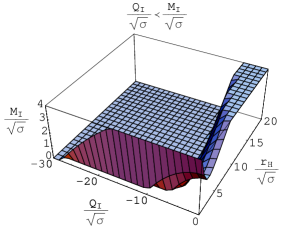
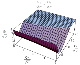
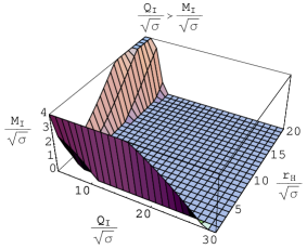
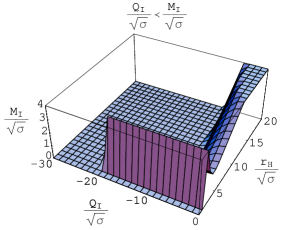
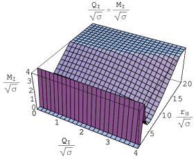
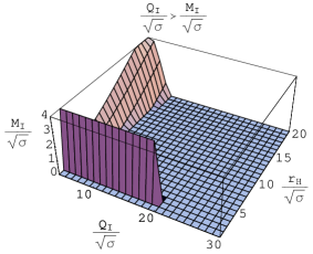
Figure 10: $\frac{M_{I}}{\sqrt{\sigma}}$ versus $\frac{r_{H}}{\sqrt{\sigma}}$ for $t=0$.

Figure 11: $\frac{M_{I}}{\sqrt{\sigma}}$ versus $\frac{r_{H}}{\sqrt{\sigma}}$ for $t=1.00\sqrt{\sigma}$.

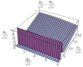
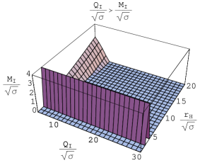
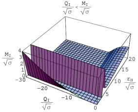
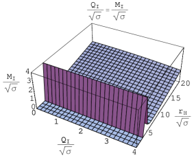
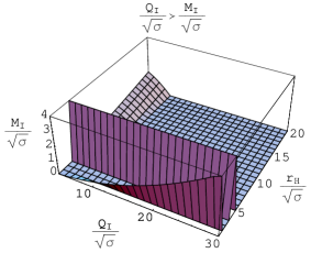
Figure 12: $\frac{M_{I}}{\sqrt{\sigma}}$ versus $\frac{r_{H}}{\sqrt{\sigma}}$ for $t=2.00\sqrt{\sigma}$.

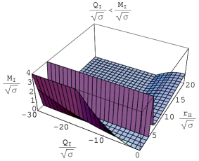
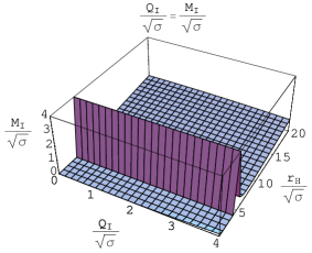
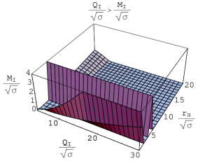
Figure 13: $\frac{M_{I}}{\sqrt{\sigma}}$ versus $\frac{r_{H}}{\sqrt{\sigma}}$ for $t=3.00\sqrt{\sigma}$.

Figure 14: $\frac{M_{I}}{\sqrt{\sigma}}$ versus $\frac{r_{H}}{\sqrt{\sigma}}$ for $t=4.00\sqrt{\sigma}$.

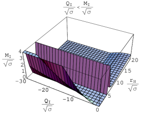
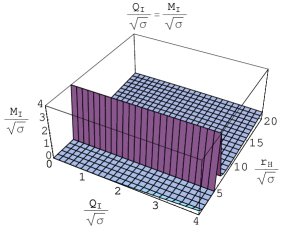
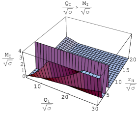
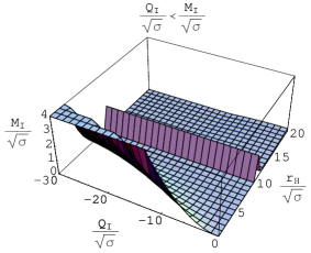
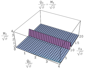
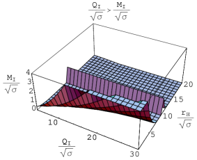
Figure 15: $\frac{M_{I}}{\sqrt{\sigma}}$ versus $\frac{r_{H}}{\sqrt{\sigma}}$ for $t=5.00\sqrt{\sigma}$.

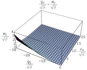
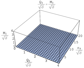
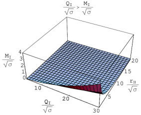
Figure 16: $\frac{M_{I}}{\sqrt{\sigma}}$ versus $\frac{r_{H}}{\sqrt{\sigma}}$ for $t=10.00\sqrt{\sigma}$.

Figure 17: $\frac{M_{I}}{\sqrt{\sigma}}$ versus $\frac{r_{H}}{\sqrt{\sigma}}$ for $t=100.00\sqrt{\sigma}$.

The NC form (34) has a coordinate singularity at the event horizon $r_{H}$, i.e.,

$$r_{H}=M_{\sigma}(t,r_{H})+\sqrt{M_{\sigma}^{2}(t,r_{H})-Q_{\sigma}^{2}(t,r_{H})}.$$ (38)

The analytical solution of this equation is not possible, however, we can analyze the results graphically. For this purpose, we substitute the values of $M_{\sigma}$ and $Q_{\sigma}$ from Eq.(35) in (38) and obtain

$$r_{H}^{2} - 2r_{H}M_{I}\left[\varepsilon\left(\frac{r_{H}-t}{2\sqrt{\sigma}}\right)\left(1+\frac{t^{2}}{2\sigma}\right)-\frac{r_{H}}{\sqrt{\sigma\pi}}e^{-\frac{(r_{H}-t)^{2}}{4\sigma}}\left(1+\frac{t}{r_{H}}\right)\right]$$ (39)

$$= -Q_{I}^{2}\left[\varepsilon^{2}\left(\frac{r_{H}-t}{2\sqrt{\sigma}}\right)-\frac{r_{H}-t}{\sqrt{2\sigma\pi}}\varepsilon\left(\frac{r_{H}-t}{\sqrt{2\sigma}}\right)\right].$$

The graphical representation of this equation, shown in Figures 10-17, is consistent with Table 1. The initial mass (greater than the remnant mass) yields three possible causal structures depending on different values of initial charge and horizon radius with the passage of time.

We can summarize the behavior as follows:

• For $\frac{Q_{I}}{\sqrt{\sigma}}<\frac{M_{I}}{\sqrt{\sigma}}$, $\frac{M_{I}}{\sqrt{\sigma}}\rightarrow 0$ as $\frac{Q_{I}}{\sqrt{\sigma}}\rightarrow\infty$ and $\frac{r_{H}}{\sqrt{\sigma}}\rightarrow\infty$.

  In this case, figures show the stable phase of the BH. As times pases, BH starts evaporation (due to charge), its mass reduces and approaches to zero for all horizon radius.

• For $\frac{Q_{I}}{\sqrt{\sigma}}=\frac{M_{I}}{\sqrt{\sigma}}$, $\frac{M_{I}}{\sqrt{\sigma}}\rightarrow 0$ for all $\frac{r_{H}}{\sqrt{\sigma}}$ and $\frac{Q_{I}}{\sqrt{\sigma}}$ at large times.

  Here we see from figures the initial stage of the BH evaporation. Black hole mass exhibits constant behavior (with the passage of time) for small range of horizon radius indicating no effect of charge. For large and due to effect of charge, BH mass approaches to zero for all horizon radius.

• For $\frac{Q_{I}}{\sqrt{\sigma}}>\frac{M_{I}}{\sqrt{\sigma}}$, $\frac{M_{I}}{\sqrt{\sigma}}\rightarrow 0$ as $\frac{Q_{I}}{\sqrt{\sigma}}\rightarrow 0$ and $\frac{r_{H}}{\sqrt{\sigma}}\rightarrow\infty$.

  This case yields the final stage of the BH evaporation. As time progresses, BH evaporates completely, i.e., its mass and hence temperature approaches to zero for all horizon radius.

These results imply the BH evaporation which leads to information about the instability of the BH due to charge and hence it must include a naked singularity. The total evaporation of the BH is possible when we consider the time varying mass of the BH [1, 22].

5 Hawking Radiation as Tunneling

In this section, we examine the radiation spectrum of RN-like NC BH by quantum tunneling [4]. The tunneling is a process where a charged particle moves in dynamical geometry and passes through the horizon without any singularity. It provides the emission rate of tunneled particle and depends on the key idea of energy conservation. The mass of the BH decreases appropriately when the virtual particle is emitted. This leads to a nonzero tunneling amplitude, which satisfies original Hawking calculation [23]. In this process, the coordinate system used to eliminate coordinate singularity at the horizon, is known as Painlev$\acute{e}$ coordinate system [24]. The Painlev$\acute{e}$’s time coordinate transformation is defined as

$$dt\rightarrow dt-\frac{\sqrt{1-F(t,r)}}{F(t,r)}dr.$$ (40)

Using this transformation, the corresponding spacetime (19) can be written as

$$ds^{2} = -F(t,r)dt^{2}+2\sqrt{1-F(t,r)}dtdr+dr^{2}+r^{2}d\Omega^{2},$$

$$ds^{2} = -\left(1-\frac{2M_{\sigma}(t,r)}{r}+\frac{Q_{\sigma}^{2}(t,r)}{r^{2}}\right)dt^{2}$$ (41)

$$+ 2\sqrt{\frac{2M_{\sigma}(t,r)}{r}-\frac{Q_{\sigma}^{2}(t,r)}{r^{2}}}dtdr+dr^{2}+r^{2}d\Omega^{2}.$$

The outgoing motion (radial null geodesics, $ds^{2}=d\Omega^{2}=0$) of the massless particles takes the form

$$\frac{dr}{dt}=1-\sqrt{1-F(t,r)}.$$ (42)

For an approximate value of $F(t,r)$ (short distances at the neighborhood of the BH horizon), we expand $F(t,r)$ up to first order by using Taylor series, i.e.,

$$F(t,r)|_{t}=F(t,r_{H})|_{t}+F^{\prime}(t,r_{H})|_{t}(r-r_{H})+O((r-r_{H})^{2})|_{t}.$$ (43)

Consequently, Eq.(42) becomes

$$\frac{dr}{dt}\simeq\frac{1}{2}F^{\prime}(t,r_{H})(r-r_{H})\simeq\kappa(M_{I},Q_{I})(r-r_{H}),$$ (44)

where $\kappa(M_{I},Q_{I})\simeq\frac{1}{2}F^{\prime}(t,r_{H})$ is the surface gravity.

Now we calculate Hawking temperature of the RN-like BH. There are semiclassical methods to derive the Hawking temperature in the Vaidya BH [25]. Using $T_{H}=\frac{\kappa}{2\pi}=\frac{1}{4\pi}F^{\prime}(t,r_{H})|_{t}$, it follows that

$$T_{H} = \frac{1}{4\pi}\left[-2M\left\{\left(1+\frac{t^{2}}{2\sigma}\right)\left(\frac{e^{-\frac{(r_{H}-t)^{2}}{4\sigma}}}{r_{H}\sqrt{\pi\sigma}}-\frac{\varepsilon\left(\frac{r_{H}-t}{2\sqrt{\sigma}}\right)}{r_{H}^{2}}\right)-\frac{e^{-\frac{(r_{H}-t)^{2}}{4\sigma}}}{\sqrt{\pi\sigma}}\left(\frac{-t}{r_{H}^{2}}\right.\right.\right.$$

$$- \left.\left.\frac{(r_{H}-\frac{t^{2}}{r_{H}})}{2\sigma}\right)\right\}+Q^{2}\left\{\left(\frac{2e^{-\frac{(r_{H}-t)^{2}}{4\sigma}}}{r_{H}^{2}\sqrt{\pi\sigma}}\varepsilon\left(\frac{r_{H}-t}{2\sqrt{\sigma}}\right)-\frac{2}{r_{H}^{3}}\varepsilon^{2}\left(\frac{r_{H}-t}{2\sqrt{\sigma}}\right)\right)\right.$$

$$- \left.\left.\frac{1}{\sqrt{2\pi\sigma}}\left(\left(\frac{1}{r_{H}}-\frac{t}{r_{H}^{2}}\right)\frac{\sqrt{2e^{-\frac{(r_{H}-t)^{2}}{4\sigma}}}}{\sqrt{\pi\sigma}}+\varepsilon\left(\frac{r_{H}-t}{\sqrt{2\sigma}}\right)\left(-\frac{1}{r_{H}^{2}}-\frac{2t}{r_{H}^{3}}\right)\right)\right\}\right].$$

Figure 18: Here $Q_{I}=2.00\sqrt{\sigma}<M_{I}$.

Figure 19: Here $Q_{I}=M_{I}$.

Figure 20: Here $Q_{I}=5.00\sqrt{\sigma}>M_{I}$.

For $t=0=Q_{I}$, this reduces to the Hawking temperature of the NC Schwarzschild case [9].

Figures 18-20 show the behavior of Hawking temperature, $T_{H}\sqrt{\sigma}$ versus horizon radius, $\frac{r_{H}}{\sqrt{\sigma}}$ with fixed $M_{I}=3.00\sqrt{\sigma}$. When BH evaporates, there is no radiation and hence temperature approaches to zero. The graphs turn out to be smooth at the final stage of the BH evaporation. This can also be explained as follows. When the temperature reaches a maximum definite value at the minimal nonzero value of the horizon radius $r_{0}$, then it starts to cool down up to absolute zero and leads the mass to approach to zero. For all the three possibilities of $\frac{M_{I}}{\sqrt{\sigma}}$ and $\frac{Q_{I}}{\sqrt{\sigma}}$, i.e., $\frac{Q_{I}}{\sqrt{\sigma}}<\frac{M_{I}}{\sqrt{\sigma}}$, $\frac{Q_{I}}{\sqrt{\sigma}}=\frac{M_{I}}{\sqrt{\sigma}}$ and $\frac{Q_{I}}{\sqrt{\sigma}}>\frac{M_{I}}{\sqrt{\sigma}}$, the graphs of Hawking temperature give the following behavior.

• For $\frac{Q_{I}}{\sqrt{\sigma}}<\frac{M_{I}}{\sqrt{\sigma}}$, the behavior of curves are the same as for the Schwarzschild case [18].

• For $\frac{Q_{I}}{\sqrt{\sigma}}=\frac{M_{I}}{\sqrt{\sigma}}$, temperature increases at minimal horizon radius.

• For $\frac{Q_{I}}{\sqrt{\sigma}}>\frac{M_{I}}{\sqrt{\sigma}}$, horizon radius changes its position with increasing temperature.

Now we would like to discuss the effect of electromagnetic field on the emission rate of charged particles tunnel through the quantum horizon of the BH. Here we assume that an electromagnetic field is present outside the BH. The Lagrangian function for such a Maxwell gravity system can be defined as

$$L=L_{matt}+L_{el},$$ (46)

where $L_{el}=-\frac{1}{4}F_{ab}F^{ab}$ is the Maxwell Lagrangian function and $F^{ab}$ is the Maxwell field tensor given by

$$F^{ab}=\partial^{a}\Phi^{b}-\partial^{b}\Phi^{a},$$ (47)

where $\Phi_{a}=(\Phi,0,0,0)$ is the electromagnetic 4-potential. The action and the rate of emission of a particle in tunneling process are, respectively, defined as [17]

$$I=\int_{t_{in}}^{t_{out}}(L_{matt}-p_{\Phi}\dot{\Phi})dt,\quad\Gamma\sim\exp({\textmd{-2Im}\textit{I}}),$$ (48)

where $p_{\Phi}$ is the canonical momentum conjugate to $\Phi$. In the tunneling process, the imaginary part of the amplitude for an $s$-wave, representing the outgoing positive energy particles which cross the horizon outward from $r_{in}$ to $r_{out}$, is given by

$${\textmd{Im}\textit{I}}=\textmd{Im}\int_{r_{in}}^{r_{out}}\left(p_{r}-\frac{p_{\Phi}\dot{\Phi}}{\dot{r}}\right)dr=\textmd{Im}\int_{r_{in}}^{r_{out}}\left[\int_{(0,0)}^{(p_{r},p_{\Phi})}dp^{\prime}_{r}-\frac{\dot{\Phi}}{\dot{r}}dp^{\prime}_{\Phi}\right]dr.$$ (49)

Hamilton’s equations of motion,

$$\frac{dr}{dt} = \frac{dH}{dp_{r}}|_{(r;\Phi,p_{\Phi})}=\frac{d(M-E)}{dp_{r}}=-\frac{dE}{dp_{r}},$$

$$\frac{d\Phi}{dt} = \frac{dH}{dp_{\Phi}}|_{(\Phi;r,p_{r})}=\Phi(Q-q)\frac{dq}{dp_{\Phi}},$$ (50)

provide the following relation of momentum and energy,

$${\textmd{Im}\textit{I}}=\textmd{Im}\int_{r_{in}}^{r_{out}}\left[\int_{(0,0)}^{(H,q)}\frac{dH^{\prime}}{\dot{r}}-\frac{\Phi(Q-q^{\prime})}{\dot{r}}dq^{\prime}\right]dr.$$ (51)

In this process, particles and antiparticles can be described as a positive and negative energy solution of the wave equation respectively. Black hole accretes a small negative energy, which decreases its mass. Replacing $M_{I}$ by $M_{I}-E$, $Q_{I}$ by $Q_{I}-q$ and substituting Eq.(44) in (51), we get

ImI $$= -\textmd{Im}\int_{r_{in}}^{r_{out}}\left[\int_{(0,0)}^{(E,q)}\frac{dE^{\prime}}{\kappa(M_{I}-E^{\prime},Q_{I}-q^{\prime})(r-r_{H})}\right.$$ (52)

$$+ \left.\frac{\Phi(Q-q^{\prime})dq^{\prime}}{\kappa(M_{I}-E^{\prime},Q_{I}-q^{\prime})(r-r_{H})}\right]dr.$$

This integral has a pole at the horizon $r_{H}$. To avoid this pole, we perform contour integration with the condition $r_{in}>r_{out}$ and obtain

ImI $$= -\textmd{Im}\left[\int_{(0,0)}^{(E,q)}\frac{dE^{\prime}}{\kappa(M_{I}-E^{\prime},Q_{I}-q^{\prime})}+\frac{\Phi(Q-q^{\prime})dq^{\prime}}{\kappa(M_{I}-E^{\prime},Q_{I}-q^{\prime})}\right]$$ (53)

$$\times \int_{r_{in}}^{r_{out}}\frac{dr}{r-r_{H}}$$

$$= \pi\left[\int_{(0,0)}^{(E,q)}\frac{dE^{\prime}}{\kappa(M_{I}-E^{\prime},Q_{I}-q^{\prime})}+\frac{\Phi(Q-q^{\prime})dq^{\prime}}{\kappa(M_{I}-E^{\prime},Q_{I}-q^{\prime})}\right].$$

This shows that the particles rate of emission is proportional to the surface gravity.

Using the first law of BH thermodynamics, $dM=TdS-\Phi dQ$, the imaginary part of the action ImI is given by [26]

$${\textmd{Im}\textit{I}}=-\frac{1}{2}\int_{S_{NC}(M,Q)}^{S_{NC}(M-E,Q-q)}dS=-\frac{1}{2}\Delta S_{NC},$$ (54)

where $S_{NC}$ is the entropy of the NC BH while $\Delta{S_{NC}}$ is the difference in BH entropies before and after emission. At high energies, the tunneling amplitude (emission rate) depends on the final and initial number of microstates available to the system [27]-[30] implying that the emission rate is proportional to $\exp(\Delta S_{NC})$, i.e.,

$$\Gamma\sim\frac{e^{S_{final}}}{e^{S_{initial}}}=e^{\Delta S_{NC}}=e^{S_{NC}(M_{I}-E,Q_{I}-q)-S_{NC}(M_{I},Q_{I})}.$$ (55)

It follows that the emission spectrum cannot be precisely thermal. The modified NC tunneling amplitude $\Gamma$ can be computed if we know the analytic form of $\exp(\Delta{S_{NC}})$.

According to quantum theory, a BH is neither an absolute stationary state nor even a relative stationary state, it is an excited state of gravity. Vacuum state (excited state) generates the spontaneous emission of virtual particles. Thus the emission of charged particles by BH is physically equivalent to the spontaneous emission by an excited state [31].

6 Summary

In this paper, first of all, we have derived spherically symmetric charged Vaidya metric in RN-like form and its NC version. Noncommutativity implies a minimal nonzero mass that allows the existence of an event horizon. In order to investigate the BH horizon radius depending on time, mass and charge, we have examined the behavior of $F(t,r)$ in the form of graphs, shown in Figures 1-9 for three possible structures: (i)$~{}M_{I}>M_{0},~{}$(ii)$~{}M_{I}=M_{0},~{}$(iii)$~{}M_{I}<M_{0}$. These have further been discussed for three possibilities of initial mass and initial charge, i.e., $\frac{Q_{I}}{\sqrt{\sigma}}<\frac{M_{I}}{\sqrt{\sigma}}$, $\frac{Q_{I}}{\sqrt{\sigma}}=\frac{M_{I}}{\sqrt{\sigma}}$ and $\frac{Q_{I}}{\sqrt{\sigma}}>\frac{M_{I}}{\sqrt{\sigma}}$. The first case provides two different possible horizons. Case (ii) represents the possibility of an extremum structure with one degenerate event horizon with time in the presence of charge. The last case shows that curves do not indicate any event horizon.

In Figures 10-17, the effects of charge on the BH evaporation are shown. The relationships between mass and charge indicate three different stages of BH mass and charge which lead to evaporation of the BH. Using Table 1, we have found that BH mass approaches to zero as horizon radius tend to infinity with time. This shows that structure of stable BH remnant having capability to store information has been failed and information would disappear from our world. Hence, this leads to the evaporation of the BH and the final phase is a naked singularity. We have found that BH evaporates completely in the large time limit. We also see from these figures that the cases $\frac{Q_{I}}{\sqrt{\sigma}}<\frac{M_{I}}{\sqrt{\sigma}}$ and $\frac{Q_{I}}{\sqrt{\sigma}}>\frac{M_{I}}{\sqrt{\sigma}}$ indicate reverse behavior of each other.

The analysis of Hawking temperature (Figures 18-20) shows similar behavior as that of the Schwarzschild spacetime. In the presence of charge, temperature attains a maximum position at the minimal nonzero horizon radius. As horizon radius increases, temperature vanishes which corresponds to the BH evaporation, i.e., mass approaches to zero. Finally, we have discussed the Hawking radiation by using Parikh-Wilczek tunneling process through the quantum horizon. The emission rate has been found consistent with the unitary theory. We have extended this analysis to compute the tunneling amplitude of charged massive particles from the RN-like Vaidya BH. It is mentioned here that corrections due to NC can be considered before the BH mass approaches to the Planck mass.

It would be interesting to extend this work to the dyadosphere of a RN solution and the regular BH solutions in NC space. It would also be worthwhile to examine the behavior of thermodynamical quantities, evaporation of BH remnant and Hawking radiation as tunneling for these solutions.

Acknowledgment

We would like to thank the Higher Education Commission, Islamabad, Pakistan for its financial support through the Indigenous Ph.D. 5000 Fellowship Program Batch-IV.

References

- [1] Hawking, S.W.: Comm. Math. Phys. 43(1975)199.
- [2] Hawking, S.W.: Phys. Rev. D14(1976)2460.
- [3] Gibbons, G.W. and Hawking, S.W.: Phys. Rev. D15(1977)2752.
- [4] Parikh, M.K. and Wilczek, F.: Phys. Rev. Lett. 85(2000)5042.
- [5] Pilling, T.: Phys. Lett. B 660(2008)402.
- [6] Akhmedova, V., et al.: Phys. Lett. B 666(2008)269.
- [7] Alexeyev, S.: Class. Quantum Grav. 19(2002)4431.
- [8] Smailagic, A. and Spallucci, E.: Phys. Rev. D65(2002)107701; ibid. J. Phys. A35(2002)L363; ibid. J. Phys. A36(2003)L467; ibid. J. Phys. A36(2003)L517; ibid. J. Phys. A37(2004)7169.
- [9] Nicolini, P., Smailagic, A. and Spallucci, E.: Phys. Lett. B632(2006)547; Ansoldi, S., Nicolini, P., Smailagic, A. and Spallucci, E.: Phys. Lett. B645(2007)261; Nicolini, P.: Int. J. Mod. Phys. A24(2009)1229.
- [10] Nasseri, F.: Int. J. Mod. Phys. D15(2006)1113.
- [11] Nozari, K. and Fazlpour, B.: Mod. Phys. Lett. A22(2007)2917; ibid. Acta Physica Polonica 39(2008)1363.
- [12] Preskill, J.: arXiv:9209058; Page, D.N.: Phys. Rev. Lett. 71(1993)3743; Stephens, C.R., Hooft, G. ’t and Whiting, B.F.: Class. Quantum Grav. 11(1994)621; Strominger, A.: arXiv:9501071; Banks, T. Nucl. Phys. (Proc. Suppl.) 41(1995)21; Russo, J.G.: arXiv:0501132.
- [13] Sharif, M. and Javed, W.: J. Korean Phys. Soc. 57(2010)217.
- [14] Sharif, M. and Javed, W.: Candian J. Phys. (to appear, 2011).
- [15] Mehdipour, S.H.: Commun. Theor. Phys. 52(2009)865.
- [16] Nozari, K. and Mehdipour, S.H.: Class. Quantum Grav. 25(2008)175015.
- [17] Mehdipour, S.H.: Int. J. Mod. Phys. A25(2010)5543.
- [18] Mehdipour, S.H.: Phys. Rev. D81(2010)124049.
- [19] Farley, A.N.St.J. and D’Eath, P.D.: Gen. Relativ. Gravit. 38(2006)425.
- [20] Misner, C.W., Thorne, K.S. and Wheeler, J.A.: Gravitation (Freeman, 1973).
- [21] Vaidya, P.C.: Proc. Indian Acad. Sci. A33(1951)264.
- [22] Bekenstein, J.D.: Phys. Rev. D7(1973)2333.
- [23] Hamber, H.W.: Quantum Gravitation: The Feynman Path Integral Approach (Springer-Verlag Berlin Heidelberg, 2009).
- [24] Painlev, P.: Compt. Rend. Acad. Sci. 173(1921)677.
- [25] Siahaan, H.M. and Triyanta: Int. J. Mod. Phys. A25(2010)145; ibid. arXiv:0811.1132.
- [26] Keski-Vakkuri, E. and Kraus, P.: Nucl. Phys. B491(1997)249.
- [27] Arzano, M., Medved, A.J.M. and Vagenas, E.C.: JHEP 09(2005)037; Medved, A.J.M. and Vagenas, E.C.: Mod. Phys. Lett. A20(2005)1723.
- [28] Banerjee, R., Majhi, B.R. and Samanta, S.: Phys. Rev. D77(2008)124035; Banerjee, R., Majhi, B.R.: Phys. Lett. B662(2008)62; ibid. JHEP 06(2008)095.
- [29] Banerjee, R., Chakraborty, B., Ghosh, S., Mukherjee, P. and Samanta, S.: Found. Phys. 39(2009)1297; Banerjee, R., Majhi, B.R. and Modak, S.K.: Class. Quantum Grav. 26(2009)085010.
- [30] Massar, S. and Parentani, R.: Nucl. Phys. B575(2000)333.
- [31] Fang, L. and Ruffini, R.: Basic Concepts in Relativistic Astrophysics (World Scientific, 1983).