Super-sharp resonances in chaotic wave scattering

Abstract

Wave scattering in chaotic systems can be characterized by its spectrum of resonances, $z_{n}=E_{n}-i\frac{\Gamma_{n}}{2}$, where $E_{n}$ is related to the energy and $\Gamma_{n}$ is the decay rate or width of the resonance. If the corresponding ray dynamics is chaotic, a gap is believed to develop in the large-energy limit: almost all $\Gamma_{n}$ become larger than some $\gamma$. However, rare cases with $\Gamma<\gamma$ may be present and actually dominate scattering events. We consider the statistical properties of these super-sharp resonances. We find that their number does not follow the fractal Weyl law conjectured for the bulk of the spectrum. We also test, for a simple model, the universal predictions of random matrix theory for density of states inside the gap and the hereby derived probability distribution of gap size.

Scattering of waves in complex media is a vast area of research, from oceanography and seismology through acoustics and optics, all the way to the probability amplitude waves of quantum mechanics book1 ; book3 ; book4 ; trends . We focus our attention on the important class of systems for which the complexity is not due to the presence of randomness or impurities, but rather because the corresponding ray dynamics is chaotic. The presence of multiple scattering leads to very complicated cross-sections, with strongly overlapping resonances that, although deterministic, have apparently random positions and widths. It is not uncommon that in a given situation only the sharpest resonances are relevant, with the others providing an approximately uniform background.

For concreteness of terminology, we consider quantum mechanical systems, but our results are general. We denote resonances by $E-i\frac{\Gamma}{2}$ and call $\Gamma$ the width or the decay rate. In the large-energy limit a gap develops in the resonance spectrum: most resonances have their widths larger than $\gamma$, which is the average decay rate of the corresponding classical (ray) dynamics. This was noticed long ago gaspard , and more recently there have been attempts to prove it rigorously gap . We are interested in the rare case of states inside the gap, i.e. with $\Gamma<\gamma$, which we call super-sharp resonances.

The distribution of typical resonances in chaotic systems is conjectured to follow the so-called fractal Weyl law prl91wl2003 : their number grows with $E$ as a power law, whose exponent is related to the fractal dimension $d$ of the classical repeller, the set of rays which remain trapped in the scattering region for infinite times, both in the future and in the past gasp . In a numerical experiment with a simple model, we find that the number of super-sharp resonances, denote it by $\mathcal{N}_{SSR}$, does not follow this law. It does grow with $E$ according to a power law, but the exponent seems to be insensitive to $\gamma$ or the dimension of the repeller.

We also investigate the dependence with energy of the width of the sharpest (and usually most important) resonance. Let this be denoted $\Gamma_{0}$. As $E$ grows, it is expected to converge to $\gamma$. More natural variables are their exponentials, and we find that $e^{-\Gamma_{0}}-e^{-\gamma}$ decreases with $E$ according to a power law, whose exponent is well approximated by $d-\alpha$.

A very fruitful approach to chaotic scattering of waves is random matrix theory (RMT) rmt , in which the system’s propagator (the Green’s function of the wave equation) is replaced by a random matrix, whose spectral properties are studied statistically. The RMT prediction for the density of resonance states inside the gap was derived in density . In this work we derive the RMT prediction for the probability distribution of $e^{-\Gamma_{0}}-e^{-\gamma}$, and compare both these predictions to numerical results in a specific system.

Waves in chaotic systems can be modeled by the so-called ‘quantum maps’. These are $N\times N$ unitary matrices where $N\sim 1/\hbar$, and the large energy limit $E\to\infty$ is replaced by the limit of large dimension, $N\to\infty$. This approach has been used to study transport properties of semiconductor quantum dots brouwer , entanglement production entang , the fractal Weyl law weyl , fractal wave functions resonances ; reso2 , proximity effects due to superconductors bcs , among other phenomena. Scattering can be introduced by means of projectors. The propagator becomes a sub-unitary matrix of dimension $M<N$, and its spectrum comprises $N-M$ zero eigenvalues and $M$ resonances of the form $z_{n}=e^{-i(E_{n}-i\Gamma_{n}/2)}$.

As our dynamical model we use the kicked rotator. Its classical dynamics is determined by canonical equations of motion in discrete time,

$$q_{t+1} =q_{t}+p_{t}+\frac{K}{4\pi}\sin(2\pi q_{t})\quad({\rm mod}\;1)$$ (1)

$$p_{t+1} =p_{t}+\frac{K}{4\pi}[\sin(2\pi q_{t})+\sin(2\pi q_{t+1})]\quad({\rm mod}\;1).$$ (2)

This system is known to be fully chaotic for $K>7$, with Lyapunov exponent $\lambda\approx\ln(K/2)$. Its quantization bcs ; henning yields a $N$ dimensional unitary matrix $U$. We set equal to zero a fraction of $1-\mu$ of its columns, corresponding to a ‘hole’ in phase space. Here $\mu$ corresponds to the fraction of rays which escape the scattering region per unit time, so $\mu=e^{-\gamma}$. We do not consider very small values of $\mu$, which would correspond to widely open systems.

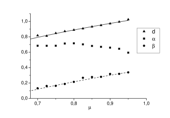
Figure 1: Scaling exponents as functions of $\mu$ for the open kicked rotator. $d$, $\alpha$ and $\beta$ are related to the fractal Weyl law, the number of super-sharp resonances and the width of the gap, respectively. We see that $\alpha$ is approximately independent of the size of the opening. The solid line is a best linear fit to $d$, while the dashed line is $d-\langle\alpha\rangle$, where $\langle\alpha\rangle\approx 0.66$ is the average value of $\alpha$.

We find numerically that $\mathcal{N}_{SSR}\sim N^{\alpha}$, while $e^{-\Gamma_{0}}-e^{-\gamma}\sim N^{-\beta}$. The exponents are plotted as functions of $\mu$ in Figure 1, together with $d$, the numerically determined exponent in the Weyl law. We see that, somewhat surprisingly, in this range $\alpha$ is approximately constant, i.e. insensitive to the dimension of the repeller. The super-sharp resonances do not follow the fractal Weyl law. On the other hand, the exponent $\beta$ has approximately the same slope as $d$. We find the relation $d-\beta=\alpha$ to be approximately fulfilled, which is to be expected since it says that the number of super-sharp resonances, $\sim N^{\alpha}$, is proportional to the total number of resonances, $\sim N^{d}$, times the width of the gap, $\sim N^{-\beta}$.

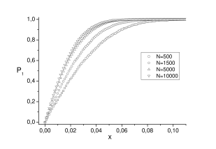
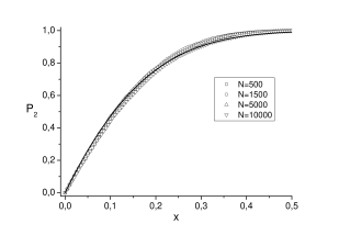
Figure 2: Top panel: $P_{1}={\rm Pr}(r^{2}-\mu<x)$ for the open kicked rotator, at several dimensions, for $\mu=0.8$. Lower panel: same for $P_{2}={\rm Pr}(\widetilde{\eta}(r^{2}-\mu)<x)$, where $\widetilde{\eta}$ is defined in the text. Solid line is a rescaled RMT prediction.

We now turn to an RMT treatment of the problem. RMT for quantum maps amounts to taking matrices uniformly distributed in the unitary group. In trunc , an ensemble of truncated unitary matrices was introduced as a model for scattering, and it was shown that, as $N,M\to\infty$ with $\mu=M/N$ held fixed, the probability density of $r=e^{-\Gamma/2}$ converges to

$$P_{\infty}(r)=\frac{1-\mu}{\mu}\frac{2r}{(1-r^{2})^{2}},$$ (3)

if $r^{2}<\mu$ and to $0$ otherwise. The expression (3) was tested numerically for a chaotic quantum map in henning and found to be an accurate description of the bulk of the spectrum, provided a rescaling was performed to incorporate the fractal Weyl law.

Let us start with the density of super-sharp resonances. This calculation can be found in density ; we sketch it here for completeness. The probability density for $r=e^{-\Gamma/2}$ is known exactly trunc , and when $M=\mu N$ and $N\gg 1$ it can be approximated to

$$P(r)\approx\frac{P_{\infty}(r)}{2}\left[1+{\rm erf}\left(\eta\sqrt{\mu}\frac{(\mu-r^{2})}{r}\right)\right],$$ (4)

where erf is the error function and

$$\eta=\sqrt{\frac{N}{2\mu(1-\mu)}}$$ (5)

is now the large number. Clearly, (4) will be different from $P_{\infty}(r)$ only if $\mu-\nu_{0}$ is of the order of $1/\eta$. After setting $r^{2}=\mu+\epsilon/\eta$, the probability distribution for the variable $\epsilon$ becomes

$$\widetilde{P}(\epsilon)=\sqrt{\pi}(1-{\rm erf}(\epsilon)).$$ (6)

This is the density of states inside the gap. It is only non-zero in a small region that shrinks as $N^{-1/2}$ in the asymptotic limit. Its integral provides the probability that $r^{2}-\mu$ be less than some value $x$. This we denote by Pr($r^{2}-\mu<x$).

In Figure 2a we see Pr($r^{2}-\mu<x$) for the open kicked rotator, at various dimensions for $\mu=0.8$. We see that as $N$ grows the values of $r$ become more localized around $\mu$. In Figure 2b we introduce a scaled variable $\widetilde{\eta}(r^{2}-\mu)$, but with $\widetilde{\eta}$ different from $\eta$ in that it involves the actual exponent $\beta$ instead of the RMT prediction $1/2$:

$$\widetilde{\eta}=\left(\frac{N}{2\mu(1-\mu)}\right)^{\beta}.$$ (7)

All curves fall on top of each other, indicating that this is the correct scaling. Moreover, the shape of the curve agrees with (6).

Let us now consider the probability distribution of the largest eigenvalue of the propagator, which corresponds to the sharpest resonance and whose modulus we denote $R$. Largest eigenvalue distributions are important in different areas of mathematics largmath and physics largphys , and have even been measured nir . A similar calculation to the one below can be found in ginibre . Let $\mathcal{P}(\{z\})$ denote the joint probability density function for all eigenvalues. When integrated over all variables from $0$ to $x$, it gives the probability that all eigenvalues are smaller than $x$. Therefore, if $Q(x)$ is the probability that the largest eigenvalue be smaller than $x$, then

$${\rm Pr}(R<x)=\int_{[0,x]^{M}}\mathcal{P}(\{z\})\prod_{i=1}^{M}d^{2}z_{i}.$$ (8)

The jpdf of the eigenvalues is trunc :

$$\mathcal{P}(\{z\})\propto\prod_{i<j}^{1..M}|z_{i}-z_{j}|^{2}\prod_{i=1}^{M}(1-|z_{i}|^{2})^{N-M-1}.$$ (9)

It is a usual trick to write $\prod_{i<j}|z_{i}-z_{j}|^{2}$ in terms of the Vandermonde determinant $|{\rm det}A|^{2}$, where $A_{ij}=z_{j}^{i-1}$. This can be shown to be equal to $M!$det$B$, where $B_{ij}=z_{i}^{j-1}(z_{i}^{*})^{i-1}$. Each element of the matrix $B$ depends on a single variable, and the integration decouples. The angular part of the integrals diagonalizes the matrix and, if $M=\mu N$ and $N\gg 1$, the result becomes

$${\rm Pr}(R<x)\propto\prod_{j=0}^{M}\int_{0}^{x}(1-y)^{N(1-\mu)}y^{j}dy.$$ (10)

This result is exact, but a bit cumbersome. Approximating the integrand by a Gaussian function we arrive at ${\rm Pr}(R<x)\propto\prod_{\ell=0}^{M}\left\{\frac{1}{2}+\frac{1}{2}{\rm erf}\left[\eta\left(x^{2}-\mu+\frac{\ell(1-\mu)}{N}\right)\right]\right\}.$ This result can be further simplified by exponentiating the product into a sum, setting the scale as $\ell=2\mu\eta\xi$ and approximating the sum by an integral. We get

$${\rm Pr}(R^{2}-\mu<x)\propto\exp\left\{2\mu\eta\int_{0}^{\infty}d\xi\mathcal{L}\left(\eta x^{2}+\xi\right)\right\},$$ (11)

where we have defined the function

$$\mathcal{L}(z)=\ln\left(\frac{1+{\rm erf}(z)}{2}\right).$$ (12)

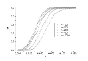
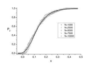
Figure 3: Top panel: $P_{1}={\rm Pr}(R^{2}-\mu<x)$, where $R$ is the modulus of the largest eigenvalue, for the open kicked rotator at several dimensions, for $\mu=0.8$. Lower panel: same for $P_{2}={\rm Pr}(\widetilde{\eta}^{2}(R^{2}-\mu)^{2}<x)$. Solid line is a rescaled RMT prediction.

One interesting question that can be answered at this point is, how likely is it that a true gap will exist at $\mu$ for a finite value of $N$? The probability that all eigenvalues are smaller than $\mu$ is simply given by the exponential in (11) with $x=0$. It is thus proportional to $e^{-c\sqrt{N}}$ for some constant $c$.

Notice that (11) has some similarity with the Tracy-Widom distribution tracy of the largest eigenvalue of Gaussian ensembles of RMT, in the sense that it involves the exponential of the integral of a function that satisfies a non-linear differential equation, $\mathcal{L}^{\prime\prime}(z)=-2z\mathcal{L}^{\prime}(z)-\left(\mathcal{L}^{\prime}(z)\right)^{2}.$ It is not a Painlevé transcendent, however.

Returning to the calculation, let us change variable to $\delta=\eta x^{2}$ and obtain $\exp\left\{2\mu\eta\int_{\delta}^{\infty}\mathcal{L}(z)dz\right\}.$ Clearly, this function does not converge as $\eta\to\infty$. Assuming $\delta$ to be large, we use $\mathcal{L}(z)\approx-e^{-z^{2}}/2\sqrt{\pi}z$ and integrate by parts to get $\exp\left\{-2\mu\eta e^{-\delta^{2}}/4\sqrt{\pi}\delta^{2}\right\}.$ In order to have a finite limit, we must have $\eta e^{-\delta^{2}}/\delta^{2}=O(1)$. This implies that $\delta^{2}=y+W{(\eta)}$, where $W$ is the Lambert function, which for large $\eta$ can be approximated as $W(\eta)\approx\log\eta-\log\log\eta$. Therefore, if instead of $R$ we consider the variable

$$\rho=\eta^{2}(R^{2}-\mu)^{2}-\log\eta+\log\log\eta,$$ (13)

then

$${\rm Pr}(\rho<y)=\exp\{-\frac{\mu}{2\sqrt{\pi}}e^{-y}\},$$ (14)

which is a modified Gumbel function. Therefore, the distribution of the slightly awkward variable $\rho$ (see also ginibre ) has a limit as $\eta\to\infty$, but this limit is approached very slowly and finite $\eta$ calculations may present significant deviations.

In Figure 3a we see Pr($R^{2}-\mu<x$) for the open kicked rotator, at various dimensions for $\mu=0.8$. In Figure 3b we introduce the scaled variable $\widetilde{\eta}^{2}(R^{2}-\mu)^{2}$, where $\widetilde{\eta}$ is given by (7). As a result, all curves fall on top of each other, indicating that this is the correct scaling. Notice that we must not introduce the $\log\widetilde{\eta}$ or $\log\log\widetilde{\eta}$ factors that appear in (13), as they would spoil the scaling. The results agree very well with the function $\exp\{-e^{-ax+b}\}$, with fitted values of $a$ and $b$.

We close with some remarks on resonance eigenfunctions. These may be depicted in phase space by means of their Husimi function, $H_{\psi}(q,p)=|\langle q,p|\psi\rangle|^{2}$, where $|q,p\rangle$ is a coherent state. It was shown in resonances that these Husimi functions are supported on the backward trapped set, the unstable manifold of the repeller. How they are distributed on this support depends on their decay rate: states with larger $\Gamma$ concentrate on the dynamical pre-images of the opening, while states with small $\Gamma$ concentrate on the repeller. Semiclassically,

$$\int_{R_{m}}H_{\psi_{n}}(q,p)dqdp\approx|z_{n}|^{2m}(1-|z_{n}|^{2}),$$ (15)

where $R_{m}$ is the $m$-th preimage of the opening. In principle, this relation would allow a state whose decay rate equals the classical decay rate to be uniformly distributed, because the area of $R_{m}$ decays like $e^{-m\gamma}$. Therefore, super-sharp resonances must show an increased degree of localization above uniformity. Indeed, since they can also be seen as super-long-lived states, one would expect them to be associated with periodic orbits (see for example old ; diego ; periodicas ; novo ). This topic deserves further investigations.

Another line of research to be followed would be to investigate a possible relation between the exponents $\alpha$ and $\beta$ to ray dynamics. In particular, it is not clear whether they depend on the Lyapounov exponent and whether they are universal or system specific.

This work was supported by CNPq and FAPESP.

References

- (1) Wave Scattering in Complex Media: From Theory to Applications, B.A. van Tiggelen and S.E. Skipetrov (Editors) (Springer, 2003).
- (2) Seismic Wave Propagation and Scattering in the Heterogenous Earth, H. Sato and M.C. Fehler (Springer, 2009).
- (3) New Directions in Linear Acoustics and Vibration: Quantum Chaos, Random Matrix Theory and Complexity, M. Wright and R. Weaver (Editors) (Cambridge University Press, 2010).
- (4) Trends in Quantum Chaotic Scattering (Special issue), J. Phys. A 38 (49), 2005.
- (5) P. Gaspard and S.A. Rice, J. Chem. Phys. 90, 2242 (1989).
- (6) S. Nonnenmacher and M. Zworski, Acta Math. 203, 149 (2009).
- (7) W.T. Lu, S. Sridhar and M. Zworski, Phys. Rev. Lett. 91, 154101 (2003).
- (8) Chaos, Scattering and Statistical Mechanics, P. Gaspard (Cambridge University Press, 2005).
- (9) Y.V. Fyodorov and H.-J. Sommers, J. Math. Phys. 38, 1918 (1997); JETP Lett. 72, 422 (2000).
- (10) B.A. Khoruzhenko and H.-J. Sommers, arXiv:math-ph/0911.5645.
- (11) S. Rahav and P.W. Brouwer, Phys. Rev. B 73, 035324 (2006).
- (12) A.J. Scott and C.M. Caves, J. Phys. A 36, 9553 (2003).
- (13) S. Nonnenmacher and M. Zworski, Commun. Math. Phys. 269, 311 (2007); D.L. Shepelyansky, Phys. Rev. E 77, 015202(R) (2008).
- (14) J.P. Keating, M. Novaes, S.D. Prado and M. Sieber, Phys. Rev. Lett. 97, 150406 (2006).
- (15) G. Casati, G. Maspero and D.L. Shepelyansky, Physica D 131, 311 (1999).
- (16) Ph. Jacquod, H. Schomerus and C.W.J. Beenakker, Phys. Rev. Lett. 90, 207004 (2003).
- (17) K. Zyczkowski and H.-J. Sommers, J. Phys. A 33, 2045 (2000).
- (18) H. Schomerus and J. Tworzydlo, Phys. Rev. Lett. 93, 154102 (2004).
- (19) C.A. Tracy and H. Widom, arXiv:math-ph/0210034v2.
- (20) S.N. Majumdar, O. Bohigas and A. Lakshminarayan, J. Stat. Phys, 131, 33 (2008).
- (21) M. Fridman, R. Pugatch, M. Nixon, A.A. Friesem and N. Davidson, arXiv:1012.1282.
- (22) B. Rider, J. Phys. A 36, 3401 (2003).
- (23) C.A. Tracy and H. Widom, Commun. Math. Phys. 159, 151 (1994).
- (24) F. Borgonovi, I. Guarnieri and D.L. Shepelyansky, Phys. Rev. A 43, 4517 (1991).
- (25) D. Wisniacki and G.G. Carlo, Phys. Rev. E 77, 045201(R) (2008).
- (26) M. Novaes, J.M. Pedrosa, D. Wisniacki, G.G. Carlo and J.P. Keating, Phys. Rev. E 80, 035202(R) (2009).
- (27) J.M. Pedrosa, D. Wisniacki, G.G. Carlo and M. Novaes, to appear.