Proportional Fair Coding for Wireless Mesh Networks

Abstract

We consider multi–hop wireless networks carrying unicast flows for multiple users. Each flow has a specified delay deadline, and the lossy wireless links are modelled as binary symmetric channels (BSCs). Since transmission time, also called airtime, on the links is shared amongst flows, increasing the airtime for one flow comes at the cost of reducing the airtime available to other flows sharing the same link. We derive the joint allocation of flow airtimes and coding rates that achieves the proportionally fair throughput allocation. This utility optimisation problem is non–convex, and one of the technical contributions of this paper is to show that the proportional fair utility optimisation can nevertheless be decomposed into a sequence of convex optimisation problems. The solution to this sequence of convex problems is the unique solution to the original non–convex optimisation. Surprisingly, this solution can be written in an explicit form that yields considerable insight into the nature of the proportional fair joint airtime/coding rate allocation. To our knowledge, this is the first time that the utility fair joint allocation of airtime/coding rate has been analysed, and also, one of the first times that utility fairness with delay deadlines has been considered.

I Introduction

In this paper, we consider wireless mesh networks with lossy links and flow delay deadlines. Packets which are decoded after a delay deadline are treated as losses. We derive the joint allocation of flow airtimes and coding rates that achieves the proportionally fair throughput allocation. To our knowledge, this is the first time that the utility fair joint allocation of airtime/coding rate has been analysed, and also, one of the first times that utility fairness with delay deadlines has been considered (also, see [1], [2]).

In the special cases where all links in a network are loss–free or all flow delay deadlines are infinite, we show that the proportionally fair utility optimisation decomposes into decoupled airtime and coding rate allocation tasks. That is, a layered approach that separates MAC scheduling and packet coding rate selection is optimal. This corresponds to the current practice, and these tasks can be solved separately using a wealth of classical techniques.

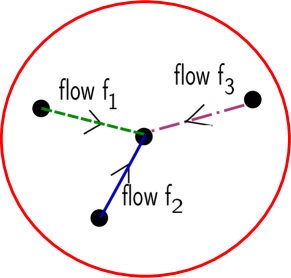
(a) Topolopgy

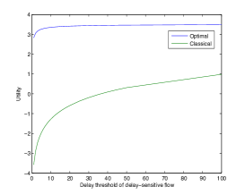
(b) Optimum Utility vs Classical Utility

Figure 1: An illustration of a single cell wireless LAN with 3 flows. The central node represents the Access Point (AP), and the other nodes represent the wireless STAtions.

However, we show that no such decomposition occurs when one or more links are lossy or, one or more flows have finite delay deadlines. Instead, in such cases, it is necessary to jointly optimise the flow airtimes and coding rates. Further, we show that the resulting allocation of airtime and coding rates is qualitatively different from classical results. For example, consider a single hop wireless network carrying three flows, see Figure 1. Flow $f_{1}$ is a delay–sensitive flow (e.g. video) while flows $f_{2}$ and $f_{3}$ are delay–insensitive flows (e.g. TCP data). Transmissions are scheduled in a TDMA manner, and the delay deadline for flow $f_{1}$ is one schedule period, while the delay deadline for flows $f_{2}$ and $f_{3}$ is infinite. The channel symbol error rate is $10^{-2}$ for all flows, and flows use MDS codes for error correction. The proportionally fair airtime and coding rate allocation that we show in this paper (see Eqns. (V-D) and (V-D)) results in the allocation of 41% of the airtime for flow $f_{1}$ while flow $f_{2}$ and flow $f_{3}$ each receive 29.5%. Observe that the proportionally fair allocation assigns unequal airtimes to the flows, which is a notable departure from the usual equal–airtime property of the proportional fair allocation when selection of delay deadlines and coding rate are not included, e.g. see [3]. The optimal coding rate is 0.62 for flow $f_{1}$ and 0.97 for flows $f_{2}$ and $f_{3}$. The coding rate for flow $f_{1}$ is much lower than for flows $f_{2}$ and $f_{3}$, since a smaller block size must be used by flow $f_{1}$ (and more redundant symbols for error–recovery) in order to respect the delay deadline. Due to the delay deadline, these optimal coding rates yield non–zero loss rates. For flow $f_{1}$, the packet loss rate at the receiver, after decoding, is 20%, whereas flows $f_{2}$ and $f_{3}$ are loss free. This highlights an important feature of the joint airtime and coding rate utility optimisation. Namely, that it allows the throughput/loss/delay trade–off amongst flows sharing network resources to be performed in a principled, fair manner. Without consideration of coding rate, the trade–off between throughput and loss cannot be fully understood or optimally managed. Without consideration of airtime, the contention between flows for shared network resources cannot be fully captured.

Proportional fairness can be formulated as a utility maximisation task, with the utility being the sum of log flow rates. Figure 1(b) compares the optimal network utility with that obtained with a classical type of approach where all flows are allocated equal airtime and the coding rates are chosen based on the channel error probabilities alone (this corresponds to ignoring the delay deadline of flow $f_{1}$). It can be seen that the optimal approach that we present in this paper potentially offers significant performance benefits over classical methods.

We note that one of the reasons why the joint selection of airtime/coding rate has not been previously studied is that the proportional fair utility optimisation is non–convex, and hence, powerful tools from convex optimisation cannot be applied directly. Also, the study of the throughput performance by jointly considering the coding and the MAC has not been performed before. One of the technical contributions of this paper is to show that the proportional fair utility optimisation can nevertheless be decomposed into a sequence of convex optimisation problems. The solution to this sequence of convex problems is the unique solution to the original non–convex optimisation. Moreover, this solution can be written in an explicit form thereby yielding considerable insight into the nature of the proportional fair airtime/coding rate allocation.

The rest of the paper is organised as follows. The related literature on utility optimal resource allocation is discussed in Section II. Section III defines the network model; in particular, we describe the mesh network architecture, the traffic model, and the channel model. We also discuss the transmission scheduling model, decoding delay deadline, and the network constraints. In Section IV, we obtain a measure for the end–to–end packet decoding error, and describe the throughput of the network. In Section V, we formulate a network utility maximisation problem subject to constraints on the transmission schedule lengths, and discuss the optimization framework. In Section VI, we discuss two special cases of networks: delay–insensitive and loss–free networks, and show that the tasks of obtaining optimal airtimes and coding rates decouple in these special cases. We discuss the optimal airtime/coding solution with some examples in Section VII. Finally we conclude in Section VIII. The proofs of Lemmas and Theorems are provided in the Appendix.

II Related Work

We consider a multi–hop Network Utility Maximisation (NUM) problem with deadline constraints and with a practical model for the PHY layer. By means of channel coding, we try to recover a packet from the channel errors. Having a low coding rate helps in recovering the packets, but at the cost of a small fraction of payload, and at the cost of the transmission airtimes of other flows. Thus, we consider the problem of resource allocation that answers the following question: how to allocate throughput across competing flows with each flow seeing different channel conditions and respecting the delay deadline.

The problem of Network Utility Maximisation (NUM) has been studied in various contexts, with NUM as a network layering tool introduced in [4].

Much of the work on NUM is concerned with the flow scheduling and throughput allocation that achieves the network stability region. This work focuses on throughput and largely ignores delay constraints. Resource allocation problems from the viewpoint of network control and stability is studied by Georgiadis et al. in [5]. Network flow scheduling problems are studied in a utility optimal framework by Shakkottai and Srikant in [6]. In all these works and the references therein, the emphasis is on the MAC layers and above. In [5], an energy optimal scheduling problem is studied in which the PHYsical layer is also considered.

Some recent work explicitly includes delay constraints in the utility optimisation. In [1], Li and Eryilmaz studied the problem of end–to–end delay constrained scheduling in multi–hop networks. They propose algorithms based on Lyapunov drift minimisation and pricing, and show that by dynamically selecting service disciplines, the proposed algorithms significantly outperform existing throughput–optimal scheduling algorithms. In [2], Jaramillo and Srikant studied a resource allocation problem in ad hoc networks with elastic and inelastic traffic with deadlines for packet reception, and obtained joint congestion control and scheduling algorithm that maximises a network utility. In this work the focus is on congestion control and scheduling, with the PHYsical layer considered to be error–free.

A short, preliminary version of the work in the current paper was presented in [7].

III Network Model

III-A Cellular Mesh Architecture

We consider networks consisting of a set of $C\geq 1$ cells, $\mathcal{C}=\{1,2,\cdots,C\}$ which define the “interference domains” in the network. We allow intra–cell interference (i.e transmissions by nodes within the same cell interfere) but assume that there is no inter–cell interference. This captures, for example, common network architectures where nodes within a given cell use the same radio channel while neighbouring cells using orthogonal radio channels. Within each cell, any two nodes are within the decoding range of each other, and hence, can communicate with each other. The cells are interconnected using multi–radio bridging nodes to create a multi–hop wireless network. A multi–radio bridging node $i$ connecting the set of cells $\mathcal{B}(i)=\{c_{1},..,c_{n}\}\subset\mathcal{C}$ can be thought of as a set of $n$ single radio nodes, one in each cell, interconnected by a high–speed, loss–free wired backplane. See, for example, Figure 2.

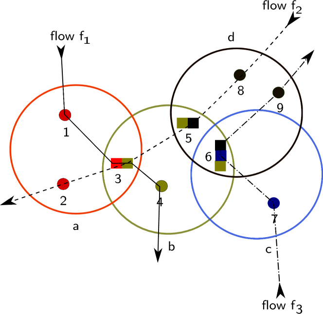
Figure 2: An illustration of a wireless mesh network with 4 cells. Cells $a$, $b$, $c$, and $d$ use orthogonal channels CH₁, CH₂, CH₃, and CH₄ respectively. Nodes 3, 5, and 6 are bridge nodes. The bridge node 3 (resp. 5 and 6) is provided a time slice of each of the channels CH₁ & CH₂ (resp. CH₂ & CH₄ for node 5 and CH₂& CH₃& CH₄ for node 6). Three flows $f_{1},f_{2}$, and $f_{3}$ are considered. In this example, $\mathcal{C}_{f_{1}}=\{a,b\}$, $\mathcal{C}_{f_{2}}=\{d,b,a\}$, and $\mathcal{C}_{f_{3}}=\{c,d\}$.

III-B Unicast Flows

Data is transmitted across this multi–hop network as a set $\mathcal{F}$ $=$ $\{1,2,\cdots,F\}$, $F\geq 1$ of unicast flows. The route of each flow $f$ $\in\mathcal{F}$ is given by $\mathcal{C}_{f}$ $=$ $\{c_{1}(f),c_{2}(f),\cdots,c_{\ell_{f}}(f)\}$, where the source node $s(f)\in c_{1}(f)$ and the destination node $d(f)\in c_{\ell_{f}}(f)$. We assume loop–free flows (i.e., no two cells in $\mathcal{C}_{f}$ are same).

III-C Binary Symmetric Channels

We associate a binary random variable $E_{f,c}[b]$ with the $b$’th bit transmitted by flow $f$ in cell $c$. $E_{f,c}[b]=0$ indicates that the bit is received correctly, and $E_{f,c}[k]=1$ indicates that the bit is received incorrectly, i.e., the bit is “flipped”. We assume that $E_{f,c}[1],E_{f,c}[2],\cdots$ are independent and identically distributed (iid), and ${\mathbb{P}}\{E_{f,c}[b]=1\}=\alpha_{f,c}\in[0,0.5)$. That is, we have a binary symmetric channel with cross-over probability $\alpha_{f,c}$. A transmitted bit may be “flipped” multiple times as it travels along the route of flow $f$, and is received incorrectly at the flow destination only if there is an odd number of such flips. The end-to-end cross-over probability along the route of flow $f$ is therefore given by

$$\alpha_{f}=\sum_{\{x_{c}\in\{0,1\},c\in\mathcal{C}_{f}:\underset{c\in\mathcal{C}_{f}}{\sum}x_{c}\ \text{is odd}\}}\ \ \prod_{c\in\mathcal{C}_{f}}\alpha_{f,c}^{x_{c}}\ \left(1-\alpha_{f,c}\right)^{1-x_{c}}.$$

Note that we can accommodate transmission of symbols from any $2^{m}=M$–ary alphabet (i.e. not just transmission of binary symbols) by associating $m$ channel uses of the BSC for every transmitted symbol. The symbol error probability (for any $m\geq 1$) is then given by $\beta_{f}=1-(1-\alpha_{f})^{m}$.

In this channel model, the channel processes across time are independent copies of the BSCs. In practice this can be realised by means of an interleaver of sufficient depth (after the channel encoder), which randomly shuffles the encoded symbols, combined with a de-interleaver (before the channel decoder) at the receiver. This interleaving and de–interleaving randomly mixes any channel fades, which can then be modelled as independent channel processes across time.

III-D Flow Transmission Scheduling

A scheduler assigns a time slice of duration $T_{f,c}>0$ time units to each flow $f$ that flows through cell $c$, subject to the constraint that $\sum_{f:c\in\mathcal{C}_{f}}T_{f,c}\leq T_{c}$ where $T_{c}$ is the period of the schedule in cell $c$. We consider a periodic scheduling strategy in which, in each cell $c$, service is given to the flows in a round robin fashion, and that each flow $f$ in cell $c$ gets a time slice of $T_{f,c}$ units in every schedule.

III-E Flow Decoding Delay Deadline

At the source node $s(f)$ for flow $f$, we assume that $k_{f}$ symbols arrive in each time slot, which allows us to simplify the analysis by ignoring queueing. Information symbols are formed into blocks of $D_{f}k_{f}$ symbols, where $D_{f}\in\{1,2,3,\cdots\}$ is the number of time slots that the block may span. Each block of $D_{f}k_{f}$ information symbols is encoded into a block of $D_{f}n_{f}$ coded symbols, where $n_{f}=k_{f}/r_{f}$ symbols, with coding rate $0<{r_{f}}\leq 1$. Here, $n_{f}$ is the number of encoded symbols transmitted in one slot i.e. the transmitted packet size. The code employed for encoding is discussed in Section IV. The quantity $D_{f}$ is a user or operator supplied quality of service parameter. It specifies the decoding delay deadline for flow $f$, since after the flow destination has collected at most $D_{f}$ successive coded packets it must attempt to decode the encoded information symbols.

III-F Network Constraints on Coding Rate

For flow $f$ in cell $c$, let $w_{f,c}$ be the rate of transmission in symbols/second, which is determined by the modulation and spectral bandwidth used for signal transmission and the within-cell FEC used. Each cell $c\in\mathcal{C}_{f}$ along the route of flow $f$ allocates an airtime of at least $\frac{n_{f}}{w_{f,c}}$ in order to transmit the packets of flow $f$. Let $\mathcal{F}_{c}:=\{f\in\mathcal{F}:c\in\mathcal{C}_{f}\}$ be the set of flows that are routed through cell $c$. We recall that the transmissions in any cell $c$ are scheduled in a TDMA fashion, and hence, the total time required for transmitting packets for all flows in cell $c$ is given by $\sum_{f\in\mathcal{F}_{c}}\frac{n_{f}}{w_{f,c}}$. Since, for cell $c$, the transmission schedule interval is $T_{c}$ units of time, the encoded packet size $n_{f}$ must satisfy the schedulability constraint

$$\sum_{f\in\mathcal{F}_{c}}\frac{n_{f}}{w_{f,c}}\leqslant T_{c}$$

Note that since we require sufficient transmit time at each cell along route $\mathcal{C}_{f}$ to allow $n_{f}$ coded symbols to be transmitted in every schedule period, there is no queueing at the cells along the route of a flow.

IV Packet Error Probability

Each transmitted symbol of flow $f$ reaches the destination node erroneously with probability $\beta_{f}$. Hence, to help protect against errors when recovering the information symbols, we encode information symbols at the source nodes using a block code (we note here that a convolutional code with zero–padding is also a block code). An $(n,k,d)$ block code has the following properties. The encoder takes a sequence of $k$ information symbols as input, and generates a sequence of $n\geq k$ coded symbols as output. The decoder takes a sequence of $n$ coded symbols as input, and outputs a sequence of $k$ information symbols. These information symbols will be error–free provided no more than $\lfloor\frac{d-1}{2}\rfloor$ of the coded symbols are corrupted. The Singleton bound [8] tells us that $d\leqslant n-k+1$, with equality for maximum–distance separable (MDS) codes. Thus, an MDS code can correct up to

$$\left\lfloor\frac{d-1}{2}\right\rfloor=\left\lfloor\frac{n-k}{2}\right\rfloor$$ (1)

errors. Examples for MDS codes include Reed–Solomon codes [8], and MDS–convolutional codes [9]. In [9], the authors show the existence of MDS–convolutional codes for any code rate. Hereafter, we will make use of Eqn. (1), and so, confine consideration to MDS codes. However, the analysis can be readily extended to other types of code provided a corresponding bound on $d$ is available.

Consider a coded block of flow $f$ and let $i\in\{1,2,\cdots,D_{f}n_{f}\}$ index the symbols in the block. Let $E_{f}[i]$ be a binary random variable which equals $0$ when the $i$’th coded symbol is received correctly and which equals $1$ when it is received corrupted. ${\mathbb{P}}\left\{E_{f}[i]=1\right\}=\beta_{f}$ and ${\mathbb{P}}\left\{E_{f}[i]=0\right\}=1-\beta_{f}$. From Eqn. (1), the probability of the block being decoded incorrectly is given by

$$\widetilde{e}_{f}={\mathbb{P}}\left\{\sum_{i=1}^{D_{f}n_{f}}E_{f}[i]>\frac{D_{f}n_{f}-D_{f}k_{f}}{2}\right\}$$

The symbol errors $E_{f}[1],\ E_{f}[2],\ \cdots,\ E_{f}[D_{f}n_{f}]$ are i.i.d. Bernoulli random variables, and so, the $\sum_{i=1}^{D_{f}n_{f}}E_{f}[i]$ is a binomial random variable. Hence, the probability of a decoding error can be computed exactly. However, the exact expression is combinatorial in nature, and is not tractable for further analysis. We therefore proceed by obtaining upper and lower bounds on the error probability, and show that the bounds are the same up to a prefactor, and that the prefactor decreases as the block size $D_{f}n_{f}$ increases. Hence, we pose the NUM based on the upper bound on the error probability. Also, we relax the following constraints: $n_{f}\in\mathbb{Z}_{+}$ and $k_{f}\in\mathbb{Z}_{+}$, and allow them to take positive real values, i.e., $n_{f}\in\mathbb{R}_{+}$ and $k_{f}\in\mathbb{R}_{+}$.

IV-A Upper and Lower Bounds

Lemma 1 (Upper Bound).

The end–to–end probability $\widetilde{e}_{f}$ of a decoding error for flow $f$ satisfies

$$\widetilde{e}_{f} \leq\ \exp\left(-D_{f}n_{f}I_{E_{f}[1]}\left(x_{f};\theta_{f}\right)\right)$$ (2)

$$=:\ e_{f}(\theta_{f},n_{f},r_{f}).$$

where $x_{f}:=\frac{1-r_{f}}{2}$, $r_{f}=k_{f}/n_{f}$ is the coding rate, $\theta_{f}>0$ is the Chernoff–bound parameter and the function $I_{Z}(x;\theta):=\theta x-\ln(\mathbb{E}\left[e^{\theta Z}\right])$ is called the rate function in large deviations theory.

Proof.

See Appendix A. ∎

Lemma 2 (Lower Bound).

The end–to–end probability $\widetilde{e}_{f}$ of a decoding error for flow $f$ satisfies

$$\widetilde{e}_{f} \geq\Gamma\exp\left(-{D_{f}n_{f}}I\left({\cal B}\left(x_{f}\right)\|{\cal B}(\beta_{f})\right)\right)$$ (3)

where

$$\Gamma=\frac{\beta_{f}}{1-\beta_{f}}\exp\left(-{D_{f}n_{f}}H\left({\cal B}\left(x_{f}\right)\right)\right)$$

and $x_{f}:=\frac{1-r_{f}}{2}$, ${\cal B}(x)$ is the Bernoulli distribution with parameter $x$, $H({\cal P})$ is the entropy of probability mass function (pmf) ${\cal P}$, and $I({\cal P}\|{\cal Q})$ is the information divergence between the pmfs ${\cal P}$ and ${\cal Q}$.

Proof.

See Appendix B. ∎

IV-B Tightness of Bounds

It can be verified that

$$I_{E_{f}[1]}\left(x_{f};\theta_{f}\right) =\theta_{f}x_{f}-\ln\left(1-\beta_{f}+\beta_{f}e^{\theta_{f}}\right)$$

Since $\theta_{f}>0$ is a free parameter, we can select the value that maximises $I_{E_{f}[1]}\left(x_{f};\theta_{f}\right)$ and so provides the tightest upper bound. It can be verified (e.g. by inspection of the second derivative) that $I_{E_{f}[1]}\left(x_{f};\theta_{f}\right)$ is concave in $\theta_{f}$ and so the KKT conditions are necessary and sufficient for an optimum. The KKT condition here is

$$\frac{\partial I_{E_{f}[1]}\left(x_{f};\theta_{f}\right)}{\partial\theta_{f}} =x_{f}-\frac{\beta_{f}e^{\theta_{f}}}{1-\beta_{f}+\beta_{f}e^{\theta_{f}}}=0$$

which is solved by

$$\theta_{f}^{*} =\ln\left(\frac{x_{f}}{\beta_{f}}\right)-\ln\left(\frac{1-x_{f}}{1-\beta_{f}}\right).$$

provided $x_{f}>\beta_{f}$. Substituting for $\theta_{f}^{*}$,

$$\max_{\theta_{f}>0}I_{E_{f}[1]}\left(x_{f};\theta_{f}\right) =I_{E_{f}[1]}\left(x_{f};\theta_{f}^{*}\right)$$

$$=x_{f}\ln\left(\frac{x_{f}}{\beta_{f}}\right)+(1-x_{f})\ln\left(\frac{1-x_{f}}{1-\beta_{f}}\right)$$

$$=I\left({\cal B}\left(x_{f}\right)\|{\cal B}(\beta_{f})\right)$$

and by Lemmas 1 and 2, the probability $\widetilde{e}_{f}$ of a decoding error satisfies

$$\Gamma e^{-{D_{f}n_{f}}I\left({\cal B}\left(x_{f}\right)\|{\cal B}(\beta_{f})\right)}\leq\widetilde{e}_{f}\leq e^{-D_{f}n_{f}I\left({\cal B}\left(x_{f}\right)\|{\cal B}(\beta_{f})\right)}.$$

It can be seen that the upper and lower bounds are the same to within prefactor $\Gamma$, and the gap between these bounds decreases exponentially as the block size $D_{f}n_{f}$ increases.

V Network Utility Optimisation

We are interested in the fair allocation of flow airtimes and coding rates amongst flows in the network. Other things being equal, we expect that decreasing the coding rate $r_{f}$ (i.e., increasing the number $D_{f}n_{f}-D_{f}k_{f}$ of redundant symbols transmitted) for flow $f$ will decrease the error probability $e_{f}$, and so increases the flow throughput. However, decreasing the coding rate increases the coded packet size $D_{f}n_{f}$, and so increases the airtime used by flow $f$. Since the network capacity is limited and shared by other flows, this generally decreases the airtime available to other flows and so decreases their throughout. Similarly, increasing the packet size $D_{f}k_{f}$ of flow $f$ increases its throughput but at the cost of increased airtime and a reduction in the throughput of other flows. We formulate this tradeoff as a utility fair optimisation problem. In particular, we focus on the proportional fair allocation since it is of wide interest and, as we will see, is tractable, despite the non–convex nature of the optimisation.

The utility fair optimisation problem is
$\displaystyle\max_{{\bm{\theta}},({\bm{n}},{\bm{x}})}\ \ \$ $\displaystyle U\left({\bm{\theta}},({\bm{n}},{\bm{x}})\right)$ (4) subject to $\displaystyle\underset{f:c\in\mathcal{C}_{f}}{\sum}\frac{n_{f}}{w_{f,c}}\leq T_{c},$ $\displaystyle\forall c\in\mathcal{C}$ (5) $\displaystyle\theta_{f}>0,$ $\displaystyle\forall f\in\mathcal{F}$ (6) $\displaystyle x_{f}\leq\overline{\lambda}_{f}\,$ $\displaystyle\forall f\in\mathcal{F}$ (7) $\displaystyle x_{f}\geq\underline{\lambda}_{f}\,$ $\displaystyle\forall f\in\mathcal{F}$ (8)
with ${\bm{\theta}}:=[\theta_{f}]_{f\in\mathcal{F}}$ the vector of Chernoff parameters, ${\bm{n}}:=[n_{f}]_{f\in\mathcal{F}}$ the vector of flow packet sizes, and ${\bm{x}}:=[x_{f}]_{f\in\mathcal{F}}$ the vector of flow coding rates (where we recall that $x_{f}=(1-r_{f})/2$). Eqn. (5) enforces the network capacity (or the flow schedulability) constraints, Eqn. (6) the positivity constraint on the Chernoff parameters, and the constraints Eqns. (7)–(8) are introduced for technical reasons that will be discussed in more detail shortly.

For proportional fairness, we select the sum of the log of the flow throughputs as our network utility $U$. For flow $f$ the expected throughput is $D_{f}k_{f}(1-\widetilde{e}_{f})$ symbols in every time interval of duration $D_{f}T_{d(f)}$ (we recall that $d(f)$ is the destination cell of flow $f$), which is the same as $k_{f}(1-\widetilde{e}_{f})$ symbols every time interval of duration $T_{d(f)}$, where $D_{f}k_{f}$ is the information packet size and $\widetilde{e}_{f}$ the packet decoding error probability. As the exact expression of $\widetilde{e}_{f}$ is intractable, we use the upper bound for $\widetilde{e}_{f}$ which is $e_{f}$. Thus, the objective function is given by

$$U\left({\bm{\theta}},({\bm{n}},{\bm{x}})\right) :=\sum_{f\in\mathcal{F}}\ln\left(k_{f}\left(1-e_{f}(\theta_{f},n_{f},x_{f})\right)\right)$$

$$=\sum_{f\in\mathcal{F}}\ln\left(n_{f}r_{f}\left(1-e_{f}(\theta_{f},n_{f},x_{f})\right)\right)$$

$$=\sum_{f\in\mathcal{F}}\ln\left(n_{f}(1-2x_{f})\left(1-e_{f}(\theta_{f},n_{f},x_{f})\right)\right)$$

$$=\sum_{f\in\mathcal{F}}\ln\left(n_{f}\right)+\sum_{f\in\mathcal{F}}\ln\left(1-2x_{f}\right)$$

$$\quad+\sum_{f\in\mathcal{F}}\ln\left(1-e_{f}(\theta_{f},n_{f},x_{f})\right).$$

The optimisation problem yields the proportional fair flow coding rates and coded packet size $n_{f}$. Since the PHY transmission rates $w_{f,c}$ are known parameters, the coded packet size is proportional to the airtime used by a flow (i.e., the airtime is given by $n_{f}/w_{f,c}$).

V-A Non–Convexity

The objective function $U({\bm{\theta}},({\bm{n}},{\bm{x}}))$ is separable in $(\theta_{f},(n_{f},x_{f}))$ for each flow $f$. However, it can be readily verified that $\ln\left(1-e_{f}(\theta_{f},n_{f},x_{f})\right)$ is not jointly concave in $(\theta_{f},(n_{f},x_{f}))$, and so, the optimisation is non–convex. Hence, the network utility maximisation problem defined in Eqns. (4)–(8) is not in the standard convex optimisation framework.

V-B Reformulation as Sequential Optimisations

We proceed by making the following key observation.

Lemma 3.

. For convex sets ${\cal Y}$ and ${\cal Z}$, and for a function $f:{\cal Y}\times{\cal Z}\to{\mathbb{R}}$ that is concave in $y\in{\cal Y}$ and in $z\in{\cal Z}$, but not jointly in $(y,z)$, the solution to the joint optimisation problem
$\displaystyle\max_{y\in{\cal Y},z\in{\cal Z}}f(y,z)$ (9) is unique, and is the same as the solution to
$\displaystyle\max_{z\in{\cal Z}}\max_{y\in{\cal Y}}f(y,z),$ (10)
if $f(y^{*}(z),z)$ is a concave function of $z$, where for each $z\in{\cal Z}$, $y^{*}(z):=\underset{y\in{\cal Y}}{\arg\max}f(y,z)$.

Proof.

See Appendix C. ∎

This lemma establishes conditions under which we can transform a non–convex optimisation into a sequence of convex optimisations. Roughly speaking, we proceed by optimising over each variable in turn and substituting the optimal variable value that is found back into the objective function. This creates a sequence of objective functions. Provided each member of this sequence is concave in the variable being optimised (but not necessary jointly concave in all variables), the solution to the sequence of convex optimisations coincides with the solution to the original non–convex optimisation. Evidently, the condition that concavity holds for every objective function in this sequence is extremely strong. Remarkably, however, we show that it is satisfied in our present network utility optimisation.

V-C Optimal ${\bm{\theta}}^{*}(x_{f})$

Taking a sequential optimisation approach, we begin by first solving the optimisation

$$\max_{{\bm{\theta}}}\ \ \ U\left({\bm{\theta}},({\bm{n}},{\bm{x}})\right)$$

subject to $$\theta_{f}>0, \forall f\in\mathcal{F}$$

given packet sizes ${\bm{n}}\in\mathbb{Z}_{+}^{F}$ and coding rates ${\bm{x}}\in[\underline{\lambda}_{f},\overline{\lambda}_{f}]^{F}$. The objective function is separable and concave in the $\theta_{f}$s. The partial derivative of $U\left({\bm{\theta}},({\bm{n}},{\bm{x}})\right)$ with respect to $\theta_{f}$ is given by

$$\frac{\partial U\left({\bm{\theta}},({\bm{n}},{\bm{x}})\right)}{\partial\theta_{f}} =\frac{e_{f}D_{f}n_{f}}{1-e_{f}}\left[x_{f}-\frac{\beta_{f}e^{\theta_{f}}}{1-\beta_{f}+\beta_{f}e^{\theta_{f}}}\right]$$ (11)

Setting this derivative equal to zero, provided $x_{f}>\beta_{f}$ this is solved by

$$\frac{\beta_{f}e^{\theta_{f}^{*}}}{1-\beta_{f}+\beta_{f}e^{\theta_{f}^{*}}} =x_{f}$$

$$\text{or},e^{\theta_{f}^{*}} =\frac{x_{f}}{\beta_{f}}\frac{1-\beta_{f}}{1-x_{f}}$$

$$\text{or},\theta_{f}^{*} =\ln\left(\frac{x_{f}}{\beta_{f}}\right)-\ln\left(\frac{1-x_{f}}{1-\beta_{f}}\right).$$ (12)

Observe that in fact $\theta_{f}^{*}$ is function only of $x_{f}$ and not both $n_{f}$ and $x_{f}$. The requirement for $x_{f}>\beta_{f}$ ensures that $\theta_{f}^{*}>0$. When $x_{f}\leq\beta_{f}$, the derivative (Eqn. (11)) is negative for all $\theta_{f}>0$. In this case, the optimum $\theta_{f}^{*}$ is zero which yields an error probability $e_{f}$ of one. Thus, for error recovery we require $x_{f}>\beta_{f}$ i.e. the coding rate $r_{f}<1-2\beta_{f}$, and for a non–empty feasible region in the NUM problem formulation in Eqns. (4)–(8) the constraints on $x_{f}$ should satisfy the following: $\overline{\lambda}_{f}<1-2\beta_{f}$ and $\underline{\lambda}_{f}>0$. We note that the capacity region for a BSC having a cross–over probability $\alpha_{f}$ with an $m$–ary signalling is $(0,m(1-H(\alpha_{f})))$, and the coding rate $1-2\beta_{f}$ lies in the capacity region.

V-D Optimal $(n_{f}^{*},x_{f}^{*})$

The next step in our sequential optimisation approach is to solve

$$\max_{({\bm{n}},{\bm{x}})}\ \ \ U\left({\bm{\theta}^{*}}({\bm{x}}),({\bm{n}},{\bm{x}})\right)$$

subject to $$\underset{f:c\in\mathcal{C}_{f}}{\sum}\frac{n_{f}}{w_{f,c}}\leq T_{c}, \forall c\in\mathcal{C}$$

$$x_{f}\leq\overline{\lambda}_{f}\, \forall f\in\mathcal{F}$$

$$x_{f}\geq\underline{\lambda}_{f}\, \forall f\in\mathcal{F}$$

That is, we substitute into the objective function for the optimal $\theta_{f}^{*}$ found in Section V-C. Defining $I_{f}=x_{f}\ln\left(\frac{x_{f}}{\beta_{f}}\right)+(1-x_{f})\ln\left(\frac{1-x_{f}}{1-\beta_{f}}\right)$,

$$U\left({\bm{\theta}^{*}}({\bm{x}}),({\bm{n}},{\bm{x}})\right) =\sum_{f\in\mathcal{F}}\ln\left(n_{f}\right)+\sum_{f\in\mathcal{F}}\ln\left(1-2x_{f}\right)$$

$$\quad+\sum_{f\in\mathcal{F}}\ln\left(1-e^{-D_{f}n_{f}I_{f}}\right).$$

It can be verified that $U\left({\bm{\theta}^{*}}({\bm{x}}),({\bm{n}},{\bm{x}})\right)$ is not jointly concave in $({\bm{n}},{\bm{x}})$. To proceed, we therefore rewrite the objective in terms of the log–transformed variables $\widetilde{n}_{f}=\ln(n_{f})$ and $\widetilde{I}_{f}=\ln(I_{f})$. Observe that the mapping from $n_{f}$ to $\widetilde{n}_{f}$ is invertible and similarly the mapping from $x_{f}$ to $\widetilde{I}_{f}$. Since $\widetilde{I}_{f}$ is a monotone increasing function of $x_{f}$ (this can be verified by inspection of the first derivative), the inverse mapping from $\widetilde{I}_{f}$ to $x_{f}$ exists and is one-to-one. With the obvious abuse of notation, we write inverse map as $x_{f}(\widetilde{I}_{f})$. In terms of these log–transformed co-ordinates, the objective function is $U\left({\bm{\theta}^{*}}({\bm{\tilde{}}{I}}),({\bm{\tilde{}}{n}},{\bm{\tilde{}}{I}})\right)$. We note that the problem defined in Eqns. (4)–(8) is equivalent to the problem,
$\displaystyle\max_{{\bm{\theta}},(\tilde{\bm{n}},\tilde{\bm{I}})}\ \ \$ $\displaystyle U\left({\bm{\theta}},({\tilde{\bm{n}}},{\tilde{\bm{I}}})\right)$ subject to $\displaystyle\underset{f:c\in\mathcal{C}_{f}}{\sum}\frac{e^{\tilde{n}_{f}}}{w_{f,c}}\leq T_{c},$ $\displaystyle\forall c\in\mathcal{C}$ (13) $\displaystyle\theta_{f}>0,$ $\displaystyle\forall f\in\mathcal{F}$ (14) $\displaystyle\tilde{I}_{f}\leq\overline{\tilde{\lambda}}_{f}\,$ $\displaystyle\forall f\in\mathcal{F}$ (15) $\displaystyle\tilde{I}_{f}\geq\underline{\tilde{\lambda}}_{f}\,$ $\displaystyle\forall f\in\mathcal{F}$ (16)
and hence, by Lemma 3, the solution to the log–transformed problem is the same as that of the problem defined in Eqns. (4)–(8). We solve the maximisation problem by convex optimisation method. We show that the objective function is jointly concave in $\left({\bm{\tilde{}}{n}},{\bm{\tilde{}}{I}}\right)$ in the following Lemma.

Lemma 4.

$$U\left({\bm{\theta}^{*}}({\bm{\tilde{}}{I}}),({\bm{\tilde{}}{n}},{\bm{\tilde{}}{I}})\right) =\sum_{f\in\mathcal{F}}\tilde{n}_{f}+\sum_{f\in\mathcal{F}}\ln\left(1-2x_{f}(\widetilde{I}_{f})\right)$$

$$\quad+\sum_{f\in\mathcal{F}}\ln\left(1-e^{-D_{f}e^{\tilde{n}_{f}+\tilde{I}_{f}}}\right).$$

is jointly concave in $\widetilde{n}_{f}$ and $\widetilde{I}_{f}$.

Proof.

See Appendix D. ∎

Hence, we have the following convex optimisation problem

$$\max_{({\bm{\tilde{}}{n}},{\bm{\tilde{}}{I}})}\ \ \ U\left({\bm{\theta}^{*}}({\bm{\tilde{}}{I}}),({\bm{\tilde{}}{n}},{\bm{\tilde{}}{I}})\right)$$ (17)

subject to $$\underset{f:c\in\mathcal{C}_{f}}{\sum}\frac{e^{\widetilde{n}_{f}}}{w_{f,c}}\leq T_{c}, \forall c\in\mathcal{C}$$ (18)

$$\tilde{I}_{f}\leq\overline{\tilde{\lambda}}_{f}\, \forall f\in\mathcal{F}$$ (19)

$$\tilde{I}_{f}\geq\underline{\tilde{\lambda}}_{f}\, \forall f\in\mathcal{F}$$ (20)

We solve the above maximisation problem using the Lagrangian relaxation approach. The Lagrangian function of the problem is given by

$$L\left(\widetilde{\bm{n}},\widetilde{\bm{I}},\bm{p},{\underline{\bm{\nu}}},{\overline{\bm{\nu}}}\right)$$

$$:=\underset{f\in\mathcal{F}}{\sum}U_{f}(\theta_{f}^{*}(\widetilde{I}_{f}),(\widetilde{n}_{f},\widetilde{I}_{f}))-\underset{c\in\mathcal{C}}{\sum}p_{c}\left(\underset{f\in\mathcal{F}_{c}}{\sum}\frac{e^{{\widetilde{n}}_{f}}}{w_{f,c}}-T_{c}\right)$$

$$-\underset{f\in\mathcal{F}}{\sum}\underline{\nu}_{f}\left(\tilde{I}_{f}-\overline{\tilde{\lambda}}_{f}\right)+\underset{f\in\mathcal{F}}{\sum}\overline{\nu}_{f}\left(\tilde{I}_{f}-\underline{\tilde{\lambda}}_{f}\right)$$

where $\bm{p}\geq{\bm{0}}$, ${\underline{\bm{\nu}}}\geq{\bm{0}}$, and ${\overline{\bm{\nu}}}\geq{\bm{0}}$ are Lagrangian multipliers corresponding to the constraints given in Eqns. (18)–(20). The channel error probabilities $\beta_{f}$s are strictly positive, and the channel coding rates are always assumed to be in the interior of the feasibility region. Hence, the constraints for the channel coding rate given in Eqns. (19), (20) are not active at the optimal point, and the Lagrangian costs $\underline{\nu}_{f}$s and ${\overline{\nu}_{f}}$s are zero. Thus, the shadow costs corresponding to these constraints will not appear in the Lagrangian relaxation.

Since the optimisation problem falls within convex optimisation framework, and the Slater condition is satisfied, strong duality holds. Hence, the KKT conditions are necessary and sufficient for optimality. Differentiating the Lagrangian with respect to $\widetilde{n}_{f}$ at $\widetilde{n}_{f}=\widetilde{n}_{f}^{*}$, and setting equal to zero yields the KKT condition

$$1+\frac{D_{f}{\exp(\widetilde{n}_{f}^{*}+\widetilde{I}_{f}^{*})}e^{-D_{f}\exp(\widetilde{n}_{f}^{*}+\widetilde{I}_{f}^{*})}}{1-e^{-D_{f}\exp(\widetilde{n}_{f}^{*}+\widetilde{I}_{f}^{*})}} =\sum_{c\in{\cal C}_{f}}\frac{p_{c}e^{\widetilde{n}_{f}^{*}}}{w_{f,c}}$$

$$\text{or},\ \ 1+\frac{D_{f}n_{f}^{*}I_{f}(x_{f}^{*})e^{-D_{f}n_{f}^{*}I_{f}(x_{f}^{*})}}{1-e^{-D_{f}n_{f}^{*}I_{f}(x_{f}^{*})}} =\sum_{c\in{\cal C}_{f}}\frac{p_{c}n_{f}^{*}}{w_{f,c}}$$ (21)

Similarly, the KKT condition for $\widetilde{I}_{f}^{*}$ is

$$\frac{D_{f}{\exp(\widetilde{n}_{f}^{*}+\widetilde{I}_{f}^{*})}e^{-D_{f}\exp(\widetilde{n}_{f}^{*}+\widetilde{I}_{f}^{*})}}{1-e^{-D_{f}\exp(\widetilde{n}_{f}^{*}+\widetilde{I}_{f}^{*})}} =\frac{2}{1-2x_{f}^{*}}\frac{I_{f}^{*}}{\theta_{f}^{*}}$$

$$\text{or},\ \ \ \frac{D_{f}n_{f}^{*}I_{f}(x_{f}^{*})e^{-D_{f}n_{f}^{*}I_{f}(x_{f}^{*})}}{1-e^{-D_{f}n_{f}^{*}I_{f}(x_{f}^{*})}} =\frac{2}{1-2x_{f}^{*}}\frac{I_{f}(x_{f}^{*})}{\theta_{f}^{*}(x_{f}^{*})}$$ (22)

Combining eqns. (V-D) and (V-D), yields

$$\sum_{c\in{\cal C}_{f}}\frac{p_{c}n_{f}^{*}}{w_{f,c}}-1 =\frac{2}{1-2x_{f}^{*}}\frac{I_{f}(x_{f}^{*})}{\theta_{f}^{*}(x_{f}^{*})}.$$ (23)

Observe that the LHS is a function of $n_{f}^{*}$ and the RHS is a function of $x_{f}^{*}$. Thus, the choice of packet size parameter $n_{f}^{*}$ and coding rate parameter $x_{f}^{*}$ are in general coupled.

V-E Distributed Algorithm for Solving Optimisation

Given the values of the Lagrange multipliers ${\bm{p}}^{*}$, the solution to Eqn. (23) specifies the optimal packet size and coding rate. To complete the solution to the optimisation it therefore remains to calculate the multipliers ${\bm{p}}^{*}$. These cannot be obtained in closed form since their values reflect the network topology and details of flow routing. However, they can be readily found in a distributed manner using a standard subgradient approach.

We proceed as follows. The dual problem for the primal problem defined in Eqn. (17) is given by

$$\min_{{\bm{p}}\geq 0} D(\bm{p}),$$

where the dual function $D(\bm{p})$ is given by

$$D(\bm{p}) =\max_{(\widetilde{\bm{n}},\widetilde{\bm{I}})}\ \sum_{f\in\mathcal{F}}\ U_{f}(\theta_{f}^{*}(\widetilde{I}_{f}),(\widetilde{n}_{f},\widetilde{I}_{f}))$$

$$\quad+\underset{c\in\mathcal{C}}{\sum}p_{c}\left(T_{c}-\underset{f\in\mathcal{F}_{c}}{\sum}\frac{e^{\widetilde{n}_{f}}}{w_{f,c}}\right)$$ (24)

$$=\underset{f\in\mathcal{F}}{\sum}\ U_{f}\left(\theta_{f}^{*}(\widetilde{I}_{f}({\bm{p}})),(\widetilde{n}_{f}^{*}({\bm{p}}),\widetilde{I}_{f}^{*}({\bm{p}}))\right)$$

$$\quad+\underset{c\in\mathcal{C}}{\sum}p_{c}\left(T_{c}-\underset{f\in\mathcal{F}_{c}}{\sum}\frac{e^{\widetilde{n}_{f}^{*}({\bm{p}})}}{w_{f,c}}\right).$$

From Eqn. (24), for any $(\widetilde{\bm{n}},\widetilde{\bm{I}})$,

$$D(\bm{p}) \geq\underset{f\in\mathcal{F}}{\sum}U_{f}(\theta_{f}^{*}(\widetilde{I}_{f}),(\widetilde{n}_{f},\widetilde{I}_{f}))+\underset{c\in\mathcal{C}}{\sum}p_{c}\left(T_{c}-\underset{f\in\mathcal{F}_{c}}{\sum}\frac{e^{\widetilde{n}_{f}}}{w_{f,c}}\right),$$

and in particular, the dual function $D({\bm{p}})$ is greater than that for $\widetilde{I}_{f}=\widetilde{I}_{f}^{*}({\widetilde{\bm{p}}})$ for some arbitrary $\widetilde{\bm{p}}$, i.e.,

$$D(\bm{p}) \geq\underset{f\in\mathcal{F}}{\sum}\ U_{f}\left(\theta_{f}^{*}(\widetilde{I}_{f}^{*}({\widetilde{\bm{p}}})),(\widetilde{n}_{f}^{*}({\widetilde{\bm{p}}}),\widetilde{I}_{f}^{*}({\widetilde{\bm{p}}}))\right)$$

$$\quad+\underset{c\in\mathcal{C}}{\sum}p_{c}\left(T_{c}-\underset{f\in\mathcal{F}_{c}}{\sum}\frac{e^{\widetilde{n}_{f}^{*}({\widetilde{\bm{p}}})}}{w_{f,c}}\right)$$

$$=D(\widetilde{\bm{p}})+\underset{c\in\mathcal{C}}{\sum}\left(p_{c}-\widetilde{p}_{c}\right)\left(T_{c}-\underset{f\in\mathcal{F}_{c}}{\sum}\frac{e^{\widetilde{n}_{f}^{*}({\widetilde{\bm{p}}})}}{w_{f,c}}\right)$$ (25)

Thus, a sub–gradient of $D(\cdot)$ at any $\widetilde{\bm{p}}$ is given by the vector

$$\left[T_{c}-\underset{f\in\mathcal{F}_{c}}{\sum}\frac{n_{f}^{*}({\widetilde{\bm{p}}})}{w_{f,c}}\right]_{c\in\mathcal{C}},$$

and the projected subgradient descent update is

$$p_{c}(i+1)=\left[p_{c}(i)-\gamma\cdot\left(T_{c}-\underset{f\in\mathcal{F}_{c}}{\sum}\frac{n_{f}^{*}({\bm{p}}(i))}{w_{f,c}}\right)\right]^{+}$$

where $\gamma>0$ is a sufficiently small stepsize, and $[f(x)]^{+}:=\max\{f(x),0\}$ ensures that the Lagrange multiplier never goes negative (see [10]).

The subgradient updates can carried out locally by each cell $c$ since the update of $p_{c}$ only requires knowledge of the packet sizes $n_{f}^{*}({\bm{p}}(i))$ of flows $f\in\mathcal{F}_{c}$ traversing cell $c$. Thus, at the beginning of each iteration $i$, the flow source nodes choose their packet sizes as $D_{f}n_{f}^{*}({\bm{p}}(i))$ and the coding rates as $1-2x_{f}^{*}({\bm{p}}(i))$, and each cell computes its cost based on the packet sizes (or equivalently the rates) of flows through it. The updated costs along the route of each flow are then fed back to the source nodes to compute the packet size and coding rate for the next iteration.

Observe that the Lagrange multiplier $p_{c}$ can be interpreted as the cost of transmitting traffic through cell $c$. The amount of service time that is available is given by $\Delta=T_{c}-\underset{f\in\mathcal{F}_{c}}{\sum}\frac{n_{f}^{*}({\bm{p}}(i))}{w_{f,c}}$. When $\Delta$ is positive and large, then the Lagrangian cost $p_{c}$ decreases rapidly (because the dual function $D(\cdot)$ is convex), and when $\Delta$ is negative, then the Lagrangian cost $p_{c}$ increases rapidly to make $\Delta\geq 0$. We note that the increase or decrease of $p_{c}$ between successive iterations is proportional to $\Delta$, the amount of service time available. Thus, the sub–gradient procedure provides a dynamic control scheme to balance the network load.

The resulting distributed implementation of the joint airtime/coding rate optimisation task is summarised in Algorithm 1.

  Each cell $c$ runs:

  loop

     1. $p_{c}(i+1)=\left[p_{c}(i)-\gamma\cdot\left(T_{c}-\underset{f\in\mathcal{F}_{c}}{\sum}\frac{n_{f}^{*}({\bm{p}}(i))}{w_{f,c}}\right)\right]^{+}$

  end loop

  The source for each flow $f$ runs:

  loop

     1. Measure $\sum_{c\in{\cal C}_{f}}\frac{p_{c}}{w_{f,c}}$, the aggregate cost of using the cells along the route of flow $f$. E.g. if each cell updates the header of transmitted packets to reflect this sum, it can then be echoed back to the source by the flow destination.

     2. Find the unique packet size $n_{f}^{*}$ and coding rate $x_{f}^{*}$ that solve (23). Since there are only two variables, a simple numerical search can be used.

  end loop

Algorithm 1 Distributed implementation of joint airtime/coding rate optimisation.

VI Two Special Cases

VI-A Delay–Insensitive Networks

Suppose the delay deadline $D_{f}\rightarrow\infty$ for all flows. For any positive bounded $n_{f}^{*}I_{f}^{*}$, i.e., $0<n_{f}^{*}I_{f}^{*}<\infty$, the LHS of Eqn. (V-D) can be written as

$$\frac{D_{f}n_{f}^{*}I_{f}^{*}e^{-D_{f}n_{f}^{*}I_{f}^{*}}}{1-e^{-D_{f}n_{f}^{*}I_{f}^{*}}} =\frac{D_{f}n_{f}^{*}I_{f}^{*}}{e^{D_{f}n_{f}^{*}I_{f}^{*}}-1}$$

$$=\frac{D_{f}n_{f}^{*}I_{f}^{*}}{\sum_{j=1}^{\infty}\frac{(D_{f}n_{f}^{*}I_{f}^{*})^{j}}{j!}}$$

$$=\frac{1}{1+\sum_{j=2}^{\infty}\frac{(D_{f}n_{f}^{*}I_{f}^{*})^{j-1}}{j!}}$$

$$\therefore\lim_{D_{f}\to\infty}\frac{D_{f}n_{f}^{*}I_{f}^{*}e^{-D_{f}n_{f}^{*}I_{f}^{*}}}{1-e^{-D_{f}n_{f}^{*}I_{f}^{*}}} =0.$$ (26)

Thus, the asymptotic optimal coding rate $x_{f}^{*}$ as the delay deadline requirement $D_{f}\to\infty$ is the solution to

$$\frac{2}{1-2x_{f}^{*}}\frac{I_{f}(x_{f}^{*})}{\theta^{*}(x_{f}^{*})}=0.$$ (27)

Since $\beta_{f}<x_{f}<1/2$, it is sufficient to find the solution to

$$\frac{I_{f}(x_{f}^{*})}{\theta^{*}(x_{f}^{*})} =0.$$

$$\text{Note that}\ \lim_{x_{f}^{*}\to\beta_{f}}\frac{I_{f}(x_{f}^{*})}{\theta^{*}(x_{f}^{*})} =0,$$

$$\text{and hence},\ \lim_{D_{f}\to\infty}x_{f}^{*} =\beta_{f}.$$ (28)

Since this is the limiting solution and $x_{f}^{*}>\beta_{f}$, one can use $x_{f}^{*}=\beta_{f}+\epsilon$ for some arbitrarily small $\epsilon>0$. Similarly, from Eqn. (V-D), the asymptotic optimal packet size $n_{f}^{*}$ as $D_{f}\to\infty$ is

$$n_{f}^{*}=\frac{1}{\sum_{c\in C_{f}}p_{c}/w_{f,c}}$$ (29)

where the multipliers $p_{c}$ are obtained, as before, by subgradient descent

$$p_{c}(i+1)=\left[p_{c}(i)-\gamma\cdot\left(T_{c}-\underset{f\in\mathcal{F}_{c}}{\sum}\frac{n_{f}^{*}({\bm{p}}(i))}{w_{f,c}}\right)\right]^{+}$$ (30)

Observe that the optimal coding rate $x_{f}^{*}=\beta_{f}+\epsilon$ which is given by the solution of Eqn. (VI-A) is determined solely by the channel error rate $\beta_{f}$ of flow $f$. It is therefore completely independent of the other network properties. In particular, it is independent of the packet size $n_{f}^{*}$ used, of the other flows sharing the network and of the network topology. Conversely, observe that the optimal packet size $n_{f}^{*}$ in Eqn. (29) and Eqn. (30) is dependent on the network topology and flow routes, but is completely independent of the error rate $\beta_{f}$ and coding rate $x_{f}$. That is, in delay–insensitive networks, the joint airtime/coding rate optimisation task breaks into separate optimal airtime allocation and optimal coding rate allocation tasks which are completely decoupled. Our optimisation therefore yields a MAC/PHY layering, whereby airtime allocation/transmission scheduling is handled by the MAC whereas coding rate selection is handled by the PHY, with no cross-layer communication. It is important to note, however, that this layering does not occur in networks where one or more flows have finite delay–deadlines; see Section VII for a more detailed discussion.

VI-B Loss-Free Networks

Suppose the channel symbol error rate $\beta_{f}=0$ for all flows. From Eqn. (12), we observe that

$$\lim_{\beta_{f}\to 0}\theta_{f}^{*} =\infty,$$ (31)

and this yields $e_{f}=0$ for all flows. The objective function in Eqn. (17) degenerates to $\sum_{f\in\mathcal{F}}\ln(n_{f}(1-2x_{f}))$. We note that for any $x^{*}_{f}>\beta_{f}>0$, as $\beta_{f}\downarrow 0$, $I_{f}(x_{f}^{*})\to\infty$. Hence, the LHS of Eqn. (V-D) becomes,

$$\lim_{\beta_{f}\downarrow 0}\frac{D_{f}n_{f}^{*}I_{f}(x_{f}^{*})e^{-D_{f}n_{f}^{*}I_{f}(x_{f}^{*})}}{1-e^{-D_{f}n_{f}^{*}I_{f}(x_{f}^{*})}} =0.$$ (32)

In the same was as in Eqn. (VI-A), this limit can be achieved by $x_{f}^{*}=0$ (i.e. $r_{f}^{*}=1$). Similarly, the optimal packet size is $n_{f}^{*}=\frac{1}{\sum_{c\in\mathcal{C}_{f}}p_{c}/w_{f,c}}$. This optimal packet size is identical to that for delay–insensitive networks, see Eqn. (29), and it can be verified that in fact it corresponds to the classical proportional fair rate allocation for loss–free networks, as expected.

VII Examples

VII-A Single cell

We begin by considering network examples consisting of a single cell carrying multiple flows. The network topology is illustrated schematically in Figure 1 and might correspond, for example, to a WLAN.

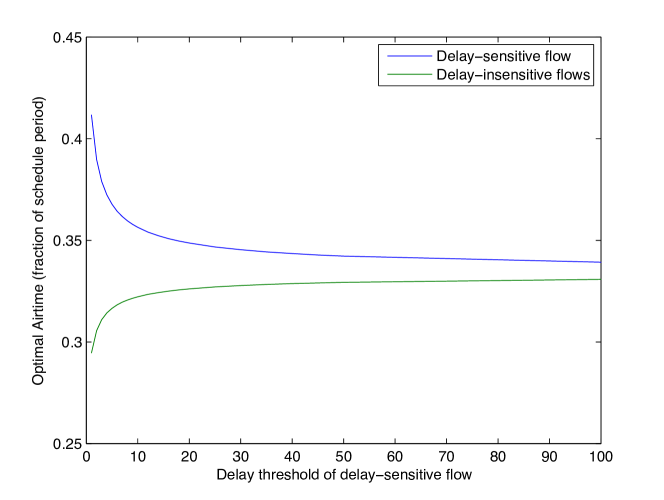
(a) Optimal airtime allocation vs delay deadline $D$, N=2.

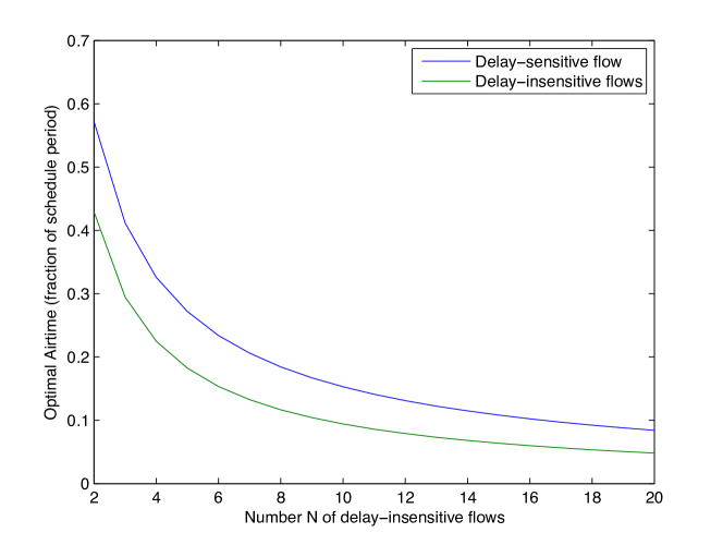
(b) Optimal airtime allocation vs N. $D=1$.

Figure 3: Single WLAN with one delay–sensitive flow and $N$ delay–insensitive flows. Delay sensitive flow has delay deadline $D$, delay–insensitive flows have infinite delay deadlines. Raw channel symbol error rate is $10^{-2}$ for all flows, PHY rate for all flows is 10 symbols per schedule period. Optimal airtimes are given as a proportion of the schedule period.

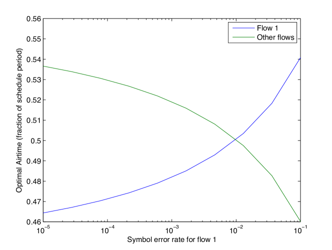
(a) Optimal airtime allocation vs channel symbol error rate for flow 1, symbol error rate for flow 2 is held fixed at $10^{-2}$.

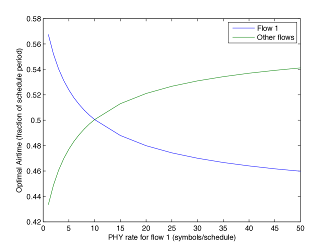
(b) Optimal airtime allocation vs PHY rate of flow 1, PHY rate for flow 2 is held fixed at 10 symbols/schedule.

Figure 4: Single WLAN with two delay–sensitive flows, both with delay deadline $D=1$. In upper figure, PHY rate for both flows is 10 symbols per schedule period and channel symbol error rate for flow 1 is varied. In lower figure, channel symbol error rate for both flows is $10^{-2}$, and PHY rate for flow 1 is varied.

VII-A1 Mix of delay–sensitive and delay–insensitive flows

Suppose the flows in the network belong to two classes, one of which is delay–sensitive and has a delay–deadline $D$ whereas the other is delay–insensitive i.e. has an infinite delay deadline. These classes might correspond, for example, to video and data traffic. Figure 3(a) plots the optimal airtime allocation as the delay deadline $D$ is varied. In this example, there is a single delay–sensitive flow and two delay–insensitive flows, and the airtime allocation is shown for the delay–sensitive flow and for one of the delay–insensitive flows (both receive the same airtime allocation). As expected, it can be seen that the airtime allocations of the delay–sensitive and delay–insensitive flows approach each other as the delay deadline $D$ is increased. However, it is notable that they approach each other fairly slowly, and when the delay deadline is low the airtime allocated to the delay–sensitive flow is almost 50% greater than that allocated to a delay–insensitive flow. This behaviour is qualitatively different from the classical proportional fair allocation neglecting coding rate and delay–deadlines, which would allocate equal airtimes to all flows. By taking coding rate and delay deadlines into account, our approach allows the resource allocation to flows with different quality of service requirements to be carried out in a principled and fair manner.

Figure 3(b) plots the optimal airtime allocation as the number $N$ of delay–insensitive flows is varied. It can be seen that the airtime allocated to each flow decreases as $N$ is increased, as expected since the number of flows sharing the network is increasing. Interestingly, observe that the airtime allocated to the delay–sensitive flow is a roughly constant margin above that allocated to the delay–insensitive flows. The delay–sensitive flow is therefore “protected” from the delay–insensitive flows. However, in contrast to ad hoc approaches, this protection is carried out in a principled and fair manner.

VII-A2 Mix of near and far stations

Consider now a situation where all flows have the same delay deadline $D$, but where for some flows the sources are located close to the destination and for other flows the sources are further away. We therefore have two classes of flows, one with a higher channel symbol error rate than the other when both use the same PHY rate. Figure 4(a) plots the optimal airtime allocation for a flow in each class as the channel error rate for one class is varied. When the channel error rates for both classes is the same ($\beta_{f}=10^{-2}$), it can be seen that the airtime allocation is the same. As the channel error rate decreases, the airtime allocated to flow 1 decreases. Conversely, as the channel error rate increases, the airtime allocated to flow 1 increases.

Figure 4(b) plots the optimal airtime allocation when flows in both classes have the same channel error rate but different PHY rates i.e. where the PHY modulation has been adjusted to equalise the channel error rates. When the PHY rates are the same ($w_{f,c}=10$ symbols per schedule period), the airtime allocation is the same to both classes. As the PHY rate is increased, the airtime allocation for flow 1 decreases. Conversely, as the PHY rate is decreased, the airtime allocation for flow 1 increases. Again, note that this is qualitatively different from the classical proportional fair allocation neglecting coding rate and delay–deadlines which would allocate equal airtimes to all flows.

VII-A3 Unequal Airtimes

The basic observations in these examples apply more generally. In particular, as noted above, in a loss-free, delay–insensitive single-cell network the proportional fair allocation is to assign equal air–time to all flows ([3] and Section VI-B). However, when delay deadlines are introduced and/or links are lossy, we see an interesting phenomenon.

Lemma 5.

The optimum rate allocation ${\bm{x}}^{*}$ (or equivalently ${\bm{r}}^{*}$) is not equivalent to an equal air–time allocation.

Proof.

See Appendix E ∎

In particular, flows that see a better channel get less air–times than flows that see a worse channel.

VII-B Multiple cells

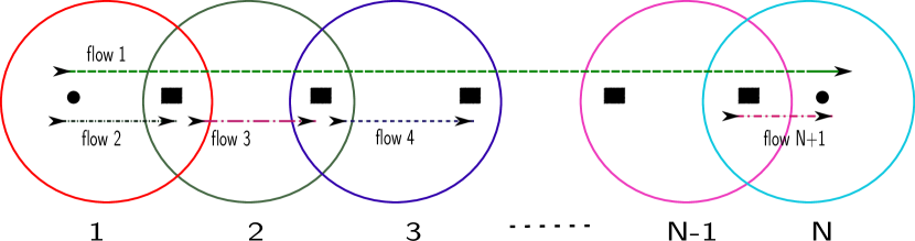
Figure 5: A linear Parking Lot network with $N$ cells and $N+1$ flows (one multi-hop flow and $N$ single-hop flows).

We now consider a mesh network consisting of $N$ cells carrying $N+1$ flows in the well-studied Parking Lot topology. The network topology is illustrated in Fig. 5. The flows in this network can be assigned to two classes: class 1 consists of the $N$-hop flow, and class 2 consists of the single–hop flows 2, 3, $\cdots$, $N+1$. Each cell has the same schedule period, i.e. $T_{c}=T,\forall c\in\mathcal{C}$.

VII-B1 Impact of number of hops

Suppose that both classes of flow use the same symbol transmission PHY rate and experience the same loss rate in each cell. Then the $N$-hop flow will experience a higher end-to-end symbol error rate that the single hop flows, and the loss rate will increase with $N$. Fig. 6 plots the ratio of optimal airtimes allocated to each class of flow versus $N$. Results are shown for three delay deadline requirements: both classes of flow are delay–sensitive with delay deadline $D_{1}=D_{2}=1$; class 1 is delay–sensitive ($D_{1}=1$) while class 2 is delay–insensitive ($D_{2}=10^{5}$); class 1 is delay–insensitive while class 2 is delay–sensitive. It can be seen that in the first case, where both classes have the same delay deadline, the ratio of airtimes is larger than 1. This is in accordance with the previous observation that flows with poorer channel conditions are allocated more airtime than flows with better channel conditions. In the second case, where class 2 is delay–insensitive ($D_{2}=10^{5}$), additional airtime is allocated to class 1, the delay–sensitive flow, which also corresponds with the single cell analysis. In the third case, where class 1 is delay–insensitive ($D_{1}=10^{5}$) and class 2 is delay–sensitive, it can be seen that class 2 flows are allocated slightly more airtime that the class 1 flow. Interestingly, however, observe that the airtime allocated to the class 1 flow is insensitive to the number $N$ of hops. This contrasts with the behaviour when the class 1 flow is delay–sensitive.

VII-B2 Impact of different flow PHY rates

Now consider a situation where the number of cells $N=3$ and all flows have the same delay deadline $D_{1}=D_{2}=1$. Flow 2 and flow 4 have symbol error rate $10^{-4}$, and flow 1 and flow 3 have symbol error rate $2.5\times 10^{-1}$. We classify the flows into three sets: class 1 consists of multi-hop flow 1, class 2 consists of single-hop flows 2 and 4, class 3 consists of single-hop flow 3. Let $w$ denote the PHY rate used used by class 1 and class 2 flows, and $w_{3}$ denote the PHY rate used by the class 3 flow. Fig. 7 plots the optimal coded packet size versus the ratio $w_{3}/w$. We begin by observing that when $w_{3}/w=1$, all flows have the same PHY rate and it can be seen that flows in classes 2 and 3 are allocated the same packet sizes (and so the same airtime). Hence, although the flow in class 3 crosses a much more lossy link than the flows in class 2, the optimal allocation ensures that all of the single-hop flows have the same airtime. The multi-hop flow in class 1 is allocated a smaller packet size (and so less airtime) than the single hop flows. It can also be seen that varying the PHY rate for the single-hop flow in class 3 does not affect the optimal coded packet sizes of flows in class 1 and class 2, and hence the airtime of class 1 and class 2 flows remains the same as $w_{3}$ is varied. The coded packet size of the class 3 flow increases linearly with $w_{3}/w$, and so the airtime of the class 4 flow remains invariant as well.

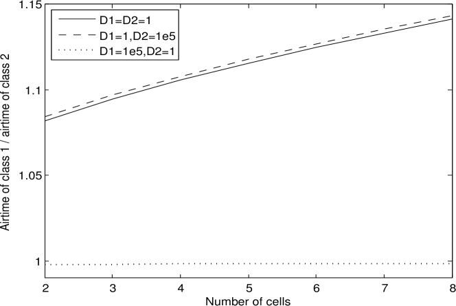
Figure 6: Ratio of airtimes vs. number $N$ of cells in Parking Lot topology of Fig. 5. The y-axis is the ratio of the airtime allocated to the $N$-hop flow to that allocated to a single hop flow; note that the airtime of the $N$-hop flow is the sum of allocated airtime in each cell along the flows route. Data is shown for three different delay deadline requirements, as indicated in the legend. All flows have the same PHY rate.

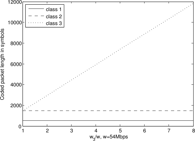
Figure 7: Coded packet size vs. ratio of PHY rates $w_{3}/w$ for Parking Lot topology of Fig. 5 with $N=3$ cells. Class 1 consists of multi-hop flow 1, class 2 consists of single-hop flows 2 and 4, class 3 consists of single-hop flow 3; class 1 and 2 flows use PHY rate $w$ bit/sec, the class 3 flow uses a PHY rate of $w_{3}$ bit/sec. All flows have delay deadline $D=1$.

VIII Conclusions

In this paper, we posed a utility fair problem that yields the optimum airtime and the coding rate across flows in a capacity constrained multi-hop network with delay deadlines. We showed that the problem is highly non–convex. Nevertheless, we demonstrate that the global network utility optimisation problem can be solved. We obtained the optimum airtime/packet size, channel coding rate, and analysed its properties. We also analysed some simple networks based on the utility optimum framework we proposed. To the best of our knowledge, this is the first work on cross–layer optimisation that studies optimum coding across flows which are competing for network resources and have delay–deadline constraints.

Appendix A Proof of Lemma 1

$$\widetilde{e}_{f} =\mathbb{P}\left\{\sum_{i=1}^{D_{f}n_{f}}E_{f}[i]>\frac{D_{f}n_{f}-D_{f}k_{f}}{2}\right\}$$

$$=\mathbb{P}\left\{\sum_{i=1}^{D_{f}n_{f}}E_{f}[i]>D_{f}n_{f}\left(\frac{1-r_{f}}{2}\right)\right\}$$

$$\leqslant\exp\left(-D_{f}n_{f}\cdot\theta_{f}\frac{1-r_{f}}{2}\right)\mathbb{E}\left[\exp\left(\theta_{f}\sum_{i=1}^{D_{f}n_{f}}E_{f}[i]\right)\right]$$

$$=\exp\left(-D_{f}n_{f}\cdot\theta_{f}\frac{1-r_{f}}{2}\right)\left[\mathbb{E}\left[\exp\bigg{(}\theta_{f}E_{f}[1]\bigg{)}\right]\right]^{D_{f}n_{f}}$$

$$=\exp\left(-D_{f}n_{f}\cdot\theta_{f}\frac{1-r_{f}}{2}\right)\exp\left(D_{f}n_{f}\ln\bigg{(}\mathbb{E}\left[e^{\theta_{f}E_{f}[1]}\right]\bigg{)}\right)$$

$$=\exp\left(-D_{f}n_{f}\left[\theta_{f}\frac{1-r_{f}}{2}-\ln\bigg{(}\mathbb{E}\left[e^{\theta_{f}E_{f}[1]}\right]\bigg{)}\right]\right)$$

$$=\exp\left(-D_{f}n_{f}I_{E_{f}[1]}\left(\frac{1-r_{f}}{2};\theta_{f}\right)\right)$$

$\hfill\blacksquare$

Appendix B Proof of Lemma 2

.

$$\widetilde{e}_{f} =\ \mathbb{P}\left\{\sum_{i=1}^{D_{f}n_{f}}E_{f}[i]>\frac{D_{f}n_{f}-D_{f}k_{f}}{2}\right\}$$

$$=\ \mathbb{P}\left\{\sum_{i=1}^{D_{f}n_{f}}E_{f}[i]>D_{f}n_{f}\frac{1-r_{f}}{2}\right\}$$

$$=\sum_{i=D_{f}n_{f}\frac{1-r_{f}}{2}+1}^{D_{f}n_{f}}{D_{f}n_{f}\choose i}\beta_{f}^{i}(1-\beta_{f})^{D_{f}n_{f}-i}.$$

The binomial coefficients can be bounded as follows:

$$1\leqslant\ {n\choose k}\ =\ \frac{n(n-1)\cdots(n-k+1)}{1\cdot 2\cdots k}\ \leqslant n^{k}.$$

Hence,

$$\widetilde{e}_{f} \geqslant\sum_{i=D_{f}n_{f}\frac{1-r_{f}}{2}+1}^{D_{f}n_{f}}\beta_{f}^{i}(1-\beta_{f})^{D_{f}n_{f}-i}$$

$$\geqslant\frac{\beta_{f}}{1-\beta_{f}}\beta_{f}^{D_{f}n_{f}(\frac{1-r_{f}}{2})}(1-\beta_{f})^{D_{f}n_{f}(\frac{1+r_{f}}{2})}$$

$$=\frac{\beta_{f}}{1-\beta_{f}}\exp\left(-D_{f}n_{f}\left[\left(\frac{1-r_{f}}{2}\right)\ln(1/\beta_{f})\right]\right)$$

$$\exp\left(-D_{f}n_{f}\left[\left(\frac{1+r_{f}}{2}\right)\ln(1/(1-\beta_{f}))\right]\right)$$

$$=\frac{\beta_{f}}{1-\beta_{f}}\exp\left(-D_{f}n_{f}\left[\left(\frac{1-r_{f}}{2}\right)\ln\left(\frac{1-r_{f}}{2\beta_{f}}\right)\right]\right)$$

$$\exp\left(-D_{f}n_{f}\left[\left(\frac{1+r_{f}}{2}\right)\ln\left(\frac{1+r_{f}}{2(1-\beta_{f})}\right)\right]\right)$$

$$\ \ \ \ \cdot\exp\left(D_{f}n_{f}\left[\left(\frac{1-r_{f}}{2}\right)\ln\left(\frac{1-r_{f}}{2}\right)\right]\right)$$

$$\cdot\exp\left(D_{f}n_{f}\left[\left(\frac{1+r_{f}}{2}\right)\ln\left(\frac{1+r_{f}}{2}\right)\right]\right)$$

$$=\frac{\beta_{f}}{1-\beta_{f}}\exp\left(-D_{f}n_{f}H\left({\cal B}\left(\frac{1-r_{f}}{2}\right)\right)\right)$$

$$\exp\left(-D_{f}n_{f}I\left({\cal B}\left(\frac{1-r_{f}}{2}\right)\|{\cal B}(\beta_{f})\right)\right)$$

$\hfill\blacksquare$

Appendix C Proof of Lemma 3

For any $z\in{\cal Z}$, the function $f(y,z)$ is concave in $y$. Hence, for each $z$, there exists a unique maximum $y^{+}(z)$, which is given by

$$f(y^{+}(z),z) = \max_{y\in{\cal Y}}\ f(y,z)$$

$$=: g(z)$$

If $f(y^{+}(z),z)$ is a concave function of $z$, then there exists a unique maximiser, which is denoted by $z^{+}$, i.e.,

$$z^{+} = \arg\max_{z\in{\cal Z}}\ f(y^{+}(z),z).$$

We show that $(y^{+}(z^{+}),z^{+})$ is an optimum solution to Eqn. (9). Since $z^{+}$ is the maximiser of $g$, we have for any $z\in{\cal Z}$,

$$g(z^{+}) \geqslant g(z)$$

$$\text{or}\ \ \ f(y^{+}(z^{+}),z^{+}) \geqslant f(y^{+}(z),z).$$

For any given $z\in{\cal Z}$, $y^{+}(z)$ is the maximiser of $f(y,z)$ over all $y\in{\cal Y}$, i.e.,

$$f(y^{+}(z),z) \geqslant f(y,z),$$

and hence, for all $(y,z)\in{\cal Y}\times{\cal Z}$,

$$f(y^{+}(z^{+}),z^{+})\ \geqslant\ f(y^{+}(z),z)\ \geqslant\ f(y,z).$$

We note that $y^{+}(\cdot)$ maps ${\cal Z}$ into ${\cal Y}$, and hence, $(y^{+}(z^{+}),z^{+})\in{\cal Y}\times{\cal Z}$. Hence, $(y^{+}(z^{+}),z^{+})$ is a global maximiser. $\hfill\blacksquare$

Appendix D Proof of Lemma 4

Consider the optimisation problem,

$$\max_{\widetilde{\bm{n}},\widetilde{\bm{I}}} \sum_{f\in\mathcal{F}}\widetilde{n}_{f}+\ln(1-2x_{f}(\widetilde{I}_{f}))+\ln(1-e^{-D_{f}\exp(\widetilde{n}_{f}+\widetilde{I}_{f})})$$

s.t. $$\sum_{f:c\in\mathcal{C}_{f}}\frac{e^{\widetilde{n}_{f}}}{w_{f,c}}\leqslant T_{c},\ \ \forall c\in\mathcal{C}$$

We show that the objective function is jointly (strictly) concave in $(\widetilde{\bm{n}},\widetilde{\bm{I}})$. The objective function is separable in $(\widetilde{n}_{f},\widetilde{I}_{f})$, and we show that $x_{f}(\widetilde{I}_{f})$ is convex, and $\ln(1-e^{-D_{f}\exp(\widetilde{n}_{f}+\widetilde{I}_{f})})$ is concave.

Since, for $x_{f}\in(\beta_{f},0.5)$, $I_{f}$ is a monotone function of $x_{f}$, and $\widetilde{I}_{f}$ is a monotone function of $I_{f}$, it is clear that $\widetilde{I}_{f}$ is invertible. Note that

$$\widetilde{I}_{f} = \ln(I_{f})$$

$$\frac{d\widetilde{I}_{f}}{dx_{f}} = \frac{\theta^{*}_{f}(x_{f})}{I_{f}}$$

$$\frac{dx_{f}}{d\widetilde{I}_{f}} = \frac{I_{f}}{\theta^{*}_{f}(x_{f})}$$

$$\frac{d^{2}x_{f}}{d\widetilde{I}_{f}^{2}} = \frac{I_{f}}{\theta^{*}_{f}(x_{f})}\left[1-\frac{I_{f}}{\theta^{*}_{f}(x_{f})^{2}}\frac{1}{x_{f}(1-x_{f})}\right]$$

Define $g(x_{f}):=x_{f}(1-x_{f})\theta_{f}^{*}(x_{f})^{2}-I_{f}$. If $g(x_{f})>0$, then $x_{f}(\widetilde{I}_{f})$ is (strictly) convex. Note that $g^{\prime}(x_{f})=(1-2x_{f})\theta_{f}^{*}(x_{f})^{2}+\theta_{f}^{*}(x_{f})$ is increasing with $x_{f}$, and hence, $g(x_{f})>g(\beta_{f})=0$.

Define $h(x,y)=e^{x+y}$. consider the function

$$f(x,y) = \ln(1-e^{-D_{f}g(x,y)})$$

$$\frac{\partial f}{\partial x} = \frac{D_{f}e^{-D_{f}g}}{1-e^{-D_{f}g}}\frac{\partial g}{\partial x}$$

$$\frac{\partial f}{\partial x} = \frac{D_{f}ge^{-D_{f}g}}{1-e^{-D_{f}g}}.$$

$$\text{Similarly,}\ \ \ \frac{\partial f}{\partial y} = \frac{D_{f}ge^{-D_{f}g}}{1-e^{-D_{f}g}}.$$

Also,

$$\frac{\partial^{2}f}{\partial x\partial y} = \frac{-D_{f}^{2}g^{2}e^{-2D_{f}g}}{(1-e^{-D_{f}g})^{2}}+\frac{D_{f}ge^{-D_{f}g}}{1-e^{-D_{f}g}}-\frac{-D_{f}^{2}g^{2}e^{-D_{f}g}}{1-e^{-D_{f}g}}$$

$$= \frac{-D_{f}g}{(1-e^{-D_{f}g})^{2}}\cdot\left[D_{f}ge^{-2D_{f}g}+\right.$$

$$\left.D_{f}g(1-e^{-D_{f}g})e^{-D_{f}g}-(1-e^{-D_{f}g})e^{-D_{f}g}\right]$$

$$= \frac{-D_{f}g}{(1-e^{-D_{f}g})^{2}}\left[D_{f}g-(1-e^{-D_{f}g})e^{-D_{f}g}\right]$$

Similarly, one can show that $\frac{\partial^{2}f}{\partial x^{2}}=\frac{\partial^{2}f}{\partial y^{2}}=\frac{\partial^{2}f}{\partial x\partial y}$. Define $\ell(x)=D_{f}x-(1-e^{-D_{f}x})e^{-D_{f}x}$. If $\ell(x)>0$, then $f(x,y)$ is (strictly) convex. Note that $\ell^{\prime}(x)=(D_{f}-D_{f}e^{-2D_{f}x})+(D_{f}e^{-D_{f}x}-D_{f}e^{-2D_{f}x})>0$. Therefore, $\ell(x)>\ell(0)=0$. $\hfill\blacksquare$

Appendix E Proof of Lemma 5

From Eqn. (V-D), it is clear that even for a single cell, because of the non–zero second term in the LHS, the air–time of flow $f$ given by $\frac{n_{f}}{w_{f,c}}$ is not the same for all the flows $f$. $\hfill\blacksquare$

References

• [1] R. Li and A. Eryilmaz, “Scheduling for end–to–end deadline–constrained traffic with reliability requirements in multi–hop networks,” in IEEE International Conference on Computer Communications (IEEE INFOCOM), Shanghai, China, Apr. 2011.
• [2] J. Jaramillo and R. Srikant, “Optimal scheduling for fair resource allocation in ad hoc networks with elastic and inelastic traffic,” IEEE/ACM Trans. Netw., vol. 19, no. 4, pp. 1125 –1136, Aug. 2011.
• [3] A. Checco and D. J. Leith, “Proportional fairness in 802.11 wireless lans,” to appear in IEEE Comm. Letters, 2011.
• [4] M. Chiang, S. H. Low, A. R. Calderbank, and J. C. Doyle, “Layering as optimization decomposition: A mathematical theory of network architectures,” Proceedings of the IEEE, vol. 95, no. 1, pp. 255 – 312, Jan. 2007.
• [5] L. Georgiadis, M. Neely, and L. Tassiulas, Resource Allocation and Cross–Layer Control in Wireless Networks.   Now Publishers Inc., Boston - Delft, 2006.
• [6] S. Shakkottai and R. Srikant, Network Optimization and Control.   Now Publishers Inc., Boston - Delft, 2008.
• [7] K. Premkumar, X. Chen, and D. J. Leith, “Utility optimal coding for packet transmission over wireless networks – Part I: Networks of binary synchronous channels,” in Forty-Ninth Annual Allerton Conference on Communication, Control, and Computing, Monticello, IL, USA, Sep. 2011.
• [8] F. J. MacWilliams and N. J. A. Sloane, The theory of error-correcting codes.   North-Holland Publishing Co., Amsderdam, 1977.
• [9] R. Smarandache, H. Gluesing-Luerssen, and J. Rosenthal, “Constructions of mds-convolutional codes,” Information Theory, IEEE Transactions on, vol. 47, no. 5, pp. 2045 –2049, jul 2001.
• [10] D. P. Bertsekas, A. Nedich, and A. E. Ozdaglar, Convex Analysis and Optimization.   Athena Scientific, Belmont, MA, 2003.