Periodic elliptic operators with asymptotically preassigned spectrum

Andrii Khrabustovskyi

Mathematical Division, B. Verkin Institute for Low Temperature Physics and Engineering of the National Academy of Sciences of Ukraine, Lenin avenue 47, Kharkiv 61103, Ukraine, tel.: +38 057 3410986
e-mail: andry9@ukr.net

Abstract. We deal with operators in $\mathbb{R}^{n}$ of the form

$$\mathbf{A}=-{1\over\mathbf{b}(x)}\sum\limits_{k=1}^{n}\displaystyle{\partial\over\partial x_{k}}\left(\mathbf{a}(x){\partial\over\partial x_{k}}\right)$$

where $\mathbf{a}(x),\mathbf{b}(x)$ are positive, bounded and periodic functions. We denote by $\mathbf{L}_{\mathrm{per}}$ the set of such operators. The main result of this work is as follows: for an arbitrary $L>0$ and for arbitrary pairwise disjoint intervals $(\alpha_{j},\beta_{j})\subset[0,L]$, $j=1,\dots,m$ ($m\in\mathbb{N}$) we construct the family of operators $\{\mathbf{A}^{\varepsilon}\in\mathbf{L}_{\mathrm{per}}\}_{\varepsilon}$ such that the spectrum of $\mathbf{A}^{\varepsilon}$ has exactly $m$ gaps in $[0,L]$ when $\varepsilon$ is small enough, and these gaps tend to the intervals $(\alpha_{j},\beta_{j})$ as $\varepsilon\to 0$. The idea how to construct the family $\left\{\mathbf{A}^{\varepsilon}\right\}_{\varepsilon}$ is based on methods of the homogenization theory.

Keywords: periodic elliptic operators, spectrum, gaps, homogenization.

Introduction

Our research is inspired by the following well-known result of Y. Colin de Verdière [4]: for arbitrary numbers $0=\lambda_{1}<\lambda_{2}<\dots<\lambda_{m}$ ($m\in\mathbb{N}$) and $n\in\mathbb{N}\setminus\left\{1\right\}$ there is a $n$-dimensional compact Riemannian manifold $M$ such that the first $m$ eigenvalues of the corresponding Laplace-Beltrami operator $-\Delta_{M}$ are exactly $\lambda_{1},\dots,\lambda_{m}$. In the work [16] we obtained an analogue of this fact for non-compact periodic manifolds: for an arbitrary $m$ pairwise disjoint finite intervals on the positive semi-axis ($m\in\mathbb{N}$) a periodic Riemannian manifold is constructed such that the spectrum of the corresponding Laplace-Beltrami operator has at least $m$ gaps, moreover the first $m$ gaps are close (in some natural sense) to these preassigned intervals.

The goal of the present work is to solve a similar problem for the following operators in $\mathbb{R}^{n}$ ($n\geq 2$):

$$\mathbf{A}=-\mathbf{b}^{-1}\mathrm{div}\left(\mathbf{a}\nabla\right)=-{1\over\mathbf{b}(x)}\sum\limits_{k=1}^{n}\displaystyle{\partial\over\partial x_{k}}\left(\mathbf{a}(x){\partial\over\partial x_{k}}\right),\quad\mathbf{a},\mathbf{b}\in\mathbf{H}_{\mathrm{per}}$$

where $\mathbf{H}_{\mathrm{per}}$ is a set of measurable real functions in $\mathbb{R}^{n}$ satisfying the conditions

$$\mathbf{f}\in\mathbf{H}_{\mathrm{per}}:\quad\begin{cases}\exists C^{-},C^{+}>0:\quad C^{-}\leq\mathbf{f}(x)\leq C^{+},\ \forall x\in\mathbb{R}^{n}&\text{(boundedness from above and form below)}\\ \forall i\in\mathbb{Z}^{n},\ \forall x\in\mathbb{R}^{n}:\quad\mathbf{f}(x+i)=\mathbf{f}(x)&\text{(periodicity)}\end{cases}$$

The operator $\mathbf{A}$ acts in the space $L_{2,\mathbf{b}}(\mathbb{R}^{n})=\left\{u\in L_{2}(\mathbb{R}^{n}),\ \|u\|^{2}_{L_{2,\mathbf{b}}(\mathbb{R}^{n})}=\int\limits_{\mathbb{R}^{n}}|u(x)|^{2}\mathbf{b}(x)dx\right\}$, it is self-adjoint and positive. We denote by $\mathbf{L}_{\mathrm{per}}$ the set of such operators.

Operators of this type occur in various areas of physics, for example in the case $n=3$ the operator $\mathbf{A}$ governs the propagation of acoustic waves in a medium with periodically varying mass density $(\mathbf{a}(x))^{-1}$ and compressibility $\mathbf{b}(x)$.

It is well-known (see e.g. [17]) that the spectrum $\sigma(\mathbf{A})$ of the operator $\mathbf{A}\in\mathbf{L}_{\mathrm{per}}$ has band structure, i.e. $\sigma(\mathbf{A})$ is the union of compact intervals $[a_{k}^{-},a_{k}^{+}]\subset[0,\infty)$ called bands ($a_{0}^{-}=0$, $a_{k}^{-}\underset{k\to\infty}{\nearrow}\infty$). In general the bands may overlap. The open interval $(\alpha,\beta)$ is called a gap if $(\alpha,\beta)\cap\sigma(\mathbf{A})=\varnothing$ and $\alpha,\beta\in\sigma(\mathbf{A})$.

The main result of this work is the following

Theorem 0.1 (Main Theorem).

Let $L>0$ be an arbitrary number and let $(\alpha_{j},\beta_{j})$ ($j={1,\dots,m},\ m\in\mathbb{N}$) be arbitrary intervals satisfying

$$0<\alpha_{1},\quad\alpha_{j}<\beta_{j}<\alpha_{j+1},\ j=\overline{1,m-1},\quad\alpha_{m}<\beta_{m}<L$$ (0.1)

Let $n\in\mathbb{N}\setminus\{1\}$.

Then one can construct the family of functions $\left\{\mathbf{a}^{\varepsilon}\in\mathbf{H}_{\mathrm{per}}\right\}_{{\varepsilon}}$ and the function $\mathbf{b}\in\mathbf{H}_{\mathrm{per}}$ such that the spectrum of the operator $\mathbf{A}^{\varepsilon}=\mathbf{b}^{-1}\mathrm{div}(\mathbf{a}^{\varepsilon}\nabla)$ has the following structure in the interval $[0,L]$ when ${\varepsilon}$ is small enough:

$$\sigma(\mathbf{A}^{\varepsilon})\cap[0,L]=[0,L]\setminus\left(\bigcup\limits_{j=1}^{m}(\alpha_{j}^{\varepsilon},\beta_{j}^{\varepsilon})\right)$$ (0.2)

where the intervals $(\alpha_{j}^{\varepsilon},\beta_{j}^{\varepsilon})$ satisfy

$$\forall j=1,\dots,m:\quad\lim\limits_{{\varepsilon}\to 0}\alpha_{j}^{\varepsilon}=\alpha_{j},\ \lim\limits_{{\varepsilon}\to 0}\beta_{j}^{\varepsilon}=\beta_{j}$$ (0.3)

Moreover, $\mathbf{a}^{\varepsilon}(x),\ \mathbf{b}(x)$ are step-functions having at most $m+1$ values.

Remark 0.1.

It follows from (0.1)-(0.3) that the operator $\mathbf{A}^{\varepsilon}$ has exactly $m$ gaps in $[0,L]$ when ${\varepsilon}$ is small enough. In general, the existence of gaps in the spectra of operators from $\mathbf{L}_{\mathrm{per}}$ is not guaranteed, for instance in the case of constant $\mathbf{a}(x)$, $\mathbf{b}(x)$ the spectrum $\sigma(\mathbf{A})$ coincides with $[0,\infty)$. Various operators from $\mathbf{L}_{\mathrm{per}}$ with gaps in their spectrum were studied in the works [6, 9, 11, 27, 7, 8, 5, 10, 22] (see also the overview [12]). In these works spectral gaps are the result of high contrast either in the coefficient $\mathbf{a}(x)$ [6, 11, 9, 27] or in the coefficient $\mathbf{b}(x)$[7, 8] or in both coefficients [5, 10, 22] (the last three works deal with the Laplace-Beltrami operator in $\mathbb{R}^{n}$ with conformally flat periodic metric; obviously, this operator belongs to $\mathbf{L}_{\mathrm{per}}$).

The operator $\mathbf{A}^{\varepsilon}$ constructed in the present work also has high contrast in the coefficients (namely, $\lim\limits_{{\varepsilon}\to 0}\left(\displaystyle{\max_{x\in\mathbb{R}^{n}}\mathbf{a}^{\varepsilon}(x)\over\min_{x\in\mathbb{R}^{n}}\mathbf{a}^{\varepsilon}(x)}\right)=\infty$), but their form essentially differs from the form of the coefficients in the works mentioned above.

The idea how to construct the functions $\mathbf{a}^{\varepsilon}(x)$, $\mathbf{b}(x)$ has come from the homogenization theory. We briefly describe this construction.

Fig. 1.

Let ${\varepsilon}>0$ be a small number. Let $G^{\varepsilon}=\bigcup\limits_{i\in\mathbb{Z}^{n}}\bigcup\limits_{j=1}^{m}G_{ij}^{\varepsilon}$ be a union of pairwise disjoint spherical shells $G_{ij}^{\varepsilon}$ lying in $\mathbb{R}^{n}$. It is supposed that the following conditions hold (see also Fig. 1):

• for any fixed $j\in\left\{1,\dots,m\right\}$ the shells $G_{ij}^{\varepsilon}$ are centered at the nodes of ${\varepsilon}$-periodic lattice in $\mathbb{R}^{n}$,

• the shells $G_{0j}^{\varepsilon}$ ($j=1,\dots,m$) belong to the cube $\left\{x=(x_{1},\dots,x_{n})\in\mathbb{R}^{n}:\ 0<x_{k}<{\varepsilon},\ \forall k\right\}$.

The external radius of the shells is equal to $r^{\varepsilon}=r{\varepsilon}$ ($r>0$), the thickness of their walls is equal to $d^{\varepsilon}={\varepsilon}^{\gamma}$ ($\gamma>3$). By $B_{ij}^{\varepsilon}$ we denote the sphere interior to $G_{ij}^{\varepsilon}$. We set $B^{\varepsilon}=\bigcup\limits_{i\in\mathbb{Z}^{n}}\bigcup\limits_{j=1}^{m}B_{ij}^{\varepsilon}$.

We define the functions $a^{\varepsilon}(x),\ b^{\varepsilon}(x)$ by the formulae

$$a^{\varepsilon}(x)=\begin{cases}1,&x\in\displaystyle\mathbb{R}^{n}\setminus G^{\varepsilon},\\ a_{j}{\varepsilon}^{\gamma+1},&x\in G_{ij}^{\varepsilon},\end{cases}\quad b^{\varepsilon}(x)=\begin{cases}1,&x\in\displaystyle\mathbb{R}^{n}\setminus\left(B^{\varepsilon}\cup G^{\varepsilon}\right),\\ b_{j},&x\in B_{ij}^{\varepsilon}\cup G_{ij}^{\varepsilon},\end{cases}$$ (0.4)

where $a_{j}$, $b_{j}$ ($j=1,\dots,m)$ are positive constants, which will be chosen later on. We consider the operator

$$\mathcal{A}^{\varepsilon}=-(b^{\varepsilon})^{-1}\mathrm{div}\left(a^{\varepsilon}\nabla\right)=-{1\over b^{\varepsilon}(x)}\sum\limits_{k=1}^{n}\displaystyle{\partial\over\partial x_{k}}\left(a^{\varepsilon}(x){\partial\over\partial x_{k}}\right)$$

It will be proved (see Theorem 1.1 below) that the spectrum of $\mathcal{A}^{\varepsilon}$ converges to the spectrum of some operator $\mathcal{A}^{0}$ acting in the Hilbert space $L_{2}(\mathbb{R}^{n})\underset{j=\overline{1,m}}{\oplus}L_{2,\rho_{j}/\sigma_{j}}(\mathbb{R}^{n})$, where $\rho_{j},\sigma_{j}$ ($j=1,\dots,m$) are positive constants. The spectrum of $\mathcal{A}^{0}$ coincides with the set $[0,\infty)\setminus\left(\bigcup\limits_{j=1}^{m}(\sigma_{j},\mu_{j})\right)$, where the intervals $(\sigma_{j},\mu_{j})$ satisfy

$$0<\sigma_{1},\quad\sigma_{j}<\mu_{j}<\sigma_{j+1},\ j=\overline{1,m-1},\quad\sigma_{m}<\mu_{m}<\infty$$

and depend in a special way on $a_{j}$ and $b_{j}$.

More precisely, we will prove that for an arbitrary $L>\mu_{k}$ the spectrum of the operator $\mathcal{A}^{\varepsilon}$ has the following structure in the interval $[0,L]$ when ${\varepsilon}$ is small enough:

$$\sigma(\mathcal{A}^{\varepsilon})\cap[0,L]=[0,L]\setminus\left(\bigcup\limits_{j=1}^{m}(\sigma_{j}^{\varepsilon},\mu_{j}^{\varepsilon})\right)$$

where the intervals $(\sigma_{j}^{\varepsilon},\mu_{j}^{\varepsilon})$ satisfy

$$\forall j=1,\dots,m:\quad\lim\limits_{{\varepsilon}\to 0}\sigma_{j}^{\varepsilon}=\sigma_{j},\quad\lim\limits_{{\varepsilon}\to 0}\mu_{j}^{\varepsilon}=\mu_{j}$$

Furthermore, we will prove (see Theorem 1.2 below) that for arbitrary intervals $(\alpha_{j},\beta_{j})$ ($j={1,\dots,m},\ m\in\mathbb{N}$) satisfying (0.1) one can choose such $a_{j}$, $b_{j}$ in (0.4) that the following equalities hold:

$$\forall j=1,\dots,m:\quad\sigma_{j}=\alpha_{j},\ \mu_{j}=\beta_{j}$$ (0.5)

Finally we set (below $y\in\mathbb{R}^{n}$)

$$\mathbf{a}^{\varepsilon}(y)={\varepsilon}^{-2}a^{\varepsilon}(x),\ \mathbf{b}(y)=b^{\varepsilon}(x),\text{ where }x=y{\varepsilon}$$

(obviously, $\mathbf{b}(y)$ is independent of ${\varepsilon}$). It is clear that $\mathbf{a}^{\varepsilon},\mathbf{b}$ belong to $\mathbf{H}_{\mathrm{per}}$ and are step-functions having at most $m+1$ values. It is easy to see that the spectra of the operator

$$\mathbf{A}^{\varepsilon}={\mathbf{b}}^{-1}\mathrm{div}({\mathbf{a}}^{\varepsilon}\nabla)$$

and the operator $\mathcal{A}^{\varepsilon}$ coincide (in fact, $\mathbf{A}^{\varepsilon}$ is obtained from $\mathcal{A}^{\varepsilon}$ via change of variables $x={y{\varepsilon}}$).

It follows from Theorem 1.1-1.2 that $\sigma(\mathbf{A}^{\varepsilon})$ satisfies (0.2)-(0.3).

We remark that the gaps open up in the spectrum of $\mathbf{A}^{\varepsilon}$ because of the high contrast in the coefficient $\mathbf{a}^{\varepsilon}(x)$. The coefficient $\mathbf{b}(x)$ is independent of ${\varepsilon}$ and it is needed only in order to control the behavior of the gaps as ${\varepsilon}\to 0$. In fact, the operator $-\mathrm{div}(\mathbf{a}^{\varepsilon}\nabla)$ also has at least $m$ gaps when ${\varepsilon}$ is small enough, but in general they do not converge to $(\alpha_{j},\beta_{j})$ as ${\varepsilon}\to 0$.

Heuristic arguments.

The classical problem of the homogenization theory (see e.g. [1, 2, 3, 18, 24, 25, 26]) is to describe the asymptotic behaviour as ${\varepsilon}\to 0$ of the operator $\mathcal{A}^{\varepsilon}$ which acts in $L_{2}(\Omega)$ ($\Omega\subset\mathbb{R}^{n}$ is a bounded domain) and is defined by the operation

$$\mathcal{A}_{\Omega}^{\varepsilon}=-\mathrm{div}\left(a^{\varepsilon}\nabla\right)$$

and either Dirichlet or Neumann boundary conditions on $\partial\Omega$. Here

$$a^{\varepsilon}(x)=\mathbf{a}(x{\varepsilon}^{-1})\text{, where }\mathbf{a}\in\mathbf{H}_{\mathrm{per}}$$ (0.6)

It is well-known that $\mathcal{A}^{\varepsilon}$ strongly resolvent converges to the operator (so-called ”homogenized operator”)

$$\mathcal{A}_{\Omega}^{0}=-\sum\limits_{k,l=1}^{n}\widehat{a}^{kl}\displaystyle{\partial^{2}\over\partial x_{k}\partial x_{l}}$$

where the constants $\widehat{a}^{kl}$ satisfy: $\exists C^{-},C^{+}>0\text{ s.t. }\forall\xi\in\mathbb{R}^{n}\ C^{-}|\xi|^{2}\leq\widehat{a}^{kl}\xi_{k}\xi_{l}\leq C^{+}|\xi|^{2}$.

It is interesting to study the asymptotic behaviour of the operator $\mathcal{A}^{\varepsilon}$ when $a^{\varepsilon}$ has more complicated form comparing with (0.6). In particular interest is the case when $a^{\varepsilon}$ is bounded below but not uniformly in ${\varepsilon}$. This is just our situation (see (0.4)): for fixed ${\varepsilon}$ one has $\min\limits_{x\in\mathbb{R}^{n}}a^{\varepsilon}(x)>0$, but $\lim\limits_{{\varepsilon}\to 0}\left(\min\limits_{x\in\mathbb{R}^{n}}a^{\varepsilon}(x)\right)=0$. Such type problems were widely studied in [18, Chapter 7]. In particular, the authors considered the operator $\mathcal{A}_{\Omega}^{D,{\varepsilon}}$ which acts in $L_{2}(\Omega)$ and is defined by the operation $\mathcal{A}_{\Omega}^{D,{\varepsilon}}=-\mathrm{div}(a^{\varepsilon}\nabla)$ and the Dirichlet boundary conditions on $\partial\Omega$. Here $\Omega\subset\mathbb{R}^{n}$ is a bounded domain, $a^{\varepsilon}$ is defined by (0.4) (only the case $m=1$ was considered). It was proved that $\mathcal{A}_{\Omega}^{D,{\varepsilon}}$ converges as ${\varepsilon}\to 0$ (in some sense which is close to strong resolvent convergence) to the operator $\mathcal{A}_{\Omega}^{D,0}$ acting in the space $L_{2}(\Omega)\oplus L_{2,\rho/\sigma}(\Omega)$ and being defined by the operation

$$\mathcal{A}_{\Omega}^{D,0}=\left(\begin{matrix}\displaystyle-\widehat{a}\Delta+\rho\ &\ -\rho\\ -\sigma\ &\ \sigma\end{matrix}\right)$$ (0.7)

and the definitional domain $\mathcal{D}(\mathcal{A}_{\Omega}^{D,0})=\left\{(u,v)\in H^{2}(\Omega)\oplus L_{2,\rho/\sigma}(\Omega):\ u|_{\partial\Omega}=0\right\}$. Here $\widehat{a},\rho,\sigma$ are positive constants that do not depend on $\Omega$. A similar result is valid for the operator $\mathcal{A}_{\Omega}^{N,{\varepsilon}}$ (the superscripts $"D"$ and $"N"$ mean Dirichlet and Neumann boundary conditions): the corresponding homogenized operator $\mathcal{A}_{\Omega}^{N,0}$ is defined by operation (0.7) and the definitional domain $\mathcal{D}(\mathcal{A}_{\Omega}^{N,0})=\left\{(u,v)\in H^{2}(\Omega)\oplus L_{2,\rho/\sigma}(\Omega):\ \left.{\partial u\over\partial n}\right|_{\partial\Omega}=0\right\}$.

Although in general the strong resolvent convergence of operators does not imply the Hausdorff convergence of their spectra (see the definition at the beginning of Section 5), but suppose for a moment that this is true for the operators $\mathcal{A}_{\Omega}^{D,{\varepsilon}}$ and $\mathcal{A}_{\Omega}^{N,{\varepsilon}}$, i.e.

$$\sigma(\mathcal{A}_{\Omega}^{D,{\varepsilon}})\underset{{\varepsilon}\to 0}{\to}\sigma(\mathcal{A}_{\Omega}^{D,0}),\ \sigma(\mathcal{A}_{\Omega}^{N,{\varepsilon}})\underset{{\varepsilon}\to 0}{\to}\sigma(\mathcal{A}_{\Omega}^{N,0})\text{ in the Hausdorff sense}$$

We denote $\Omega_{R}=\left\{x\in\mathbb{R}^{n}:\ |x|<R\right\}$. One can prove (for example, it follows from [15, Proposition 2.3]) that

$$\forall\Omega\subset\mathbb{R}^{n}:\ (\sigma,\mu)\cap\sigma(\mathcal{A}_{\Omega}^{D/N,0})=\varnothing$$

$$\forall[d^{-},d^{+}]\subset[0,\infty)\setminus(\sigma,\mu)\quad\exists R_{d}>0:\ \sigma(\mathcal{A}_{\Omega_{R}}^{D/N,0})\cap[d^{-},d^{+}]\not=\varnothing\text{ for }R>R_{d}$$

where $D/N$ is either $D$ or $N$, $\mu=\sigma+\rho$. These suggest that when ${\varepsilon}$ is small enough the operator $\mathcal{A}^{{\varepsilon}}$ has a gap in the spectrum and this gap tends to the interval $(\sigma,\mu)$ as ${\varepsilon}\to 0$.

The close problem was also considered in [21] where the authors studied the asymptotic behaviour of the attractors for semilinear hyperbolic equation ${\partial^{2}_{tt}u}+\mathcal{A}_{\Omega}^{D,{\varepsilon}}u+f^{\varepsilon}(u)=h^{\varepsilon}$.

We remark that the proof of the resolvent convergence in [18] is based on the method of so-called ”local energy characteristics”. This method is well adapted for both periodic and non-periodic operators but it is quite cumbersome. Therefore in the present work following [16] we carry out the proof in more simple fashion via the substitution of a suitable test function into the variational formulation of the spectral problem.

In the next section we describe precisely the operator $\mathcal{A}^{\varepsilon}$ and formulate Theorems 1.1-1.2. Their proofs are carried out in Sections 2-7.

1. Construction of operators $\mathcal{A}^{\varepsilon}$ and main results

Let $n\in\mathbb{N}\setminus\{1\}$, $m\in\mathbb{N}$. Let the points $x_{j}\in\mathbb{R}^{n}$ ($j=1,\dots,m$) and the number $r>0$ be such that the closed balls ${B}_{j}=\left\{x\in\mathbb{R}^{n}:\ |x-x_{j}|\leq r\right\}$ are pairwise disjoint and belong to the open cube

$${{{Y}}}=\left\{x=(x_{1},\dots,x_{n})\in\mathbb{R}^{n}:\ 0<x_{k}<1,\ \forall k\right\}$$

Let ${\varepsilon}>0$. We introduce the following notations (below $i\in\mathbb{Z}^{n}$, $j=1,\dots,m$):

$$x_{ij}^{\varepsilon}={\varepsilon}(x_{j}+i)$$

$${G}_{ij}^{\varepsilon}=\left\{x\in\mathbb{R}^{n}:\ r^{\varepsilon}-d^{\varepsilon}<|x-x_{ij}^{\varepsilon}|<r^{\varepsilon}\right\},\quad{B}_{ij}^{\varepsilon}=\left\{x\in\mathbb{R}^{n}:\ |x-x_{ij}^{\varepsilon}|<r^{\varepsilon}-d^{\varepsilon}\right\}$$

where

$$r^{\varepsilon}=r{\varepsilon},\quad d^{\varepsilon}={\varepsilon}^{\gamma},\ \gamma>3$$

We also denote

$$G^{\varepsilon}=\bigcup\limits_{i\in\mathbb{Z}^{n}}\bigcup\limits_{j=1}^{m}G_{ij}^{\varepsilon},\quad B^{\varepsilon}=\bigcup\limits_{i\in\mathbb{Z}^{n}}\bigcup\limits_{j=1}^{m}B_{ij}^{\varepsilon},\quad F^{\varepsilon}=\mathbb{R}^{n}\setminus\left(\overline{G^{\varepsilon}\cup B^{\varepsilon}}\right)$$

We define the piecewise constant functions $a^{\varepsilon}(x),\ b^{\varepsilon}(x)$ by the formulae

$$a^{\varepsilon}(x)=\begin{cases}1,&x\in F^{\varepsilon}\cup B^{\varepsilon},\\ a_{j}^{\varepsilon}\equiv a_{j}{\varepsilon}^{\gamma+1},&x\in G_{ij}^{\varepsilon}\quad(i\in\mathbb{Z}^{n},\ j=1,\dots,m),\\ \end{cases}$$ (1.1)

$$b^{\varepsilon}(x)=\begin{cases}1,&x\in F^{\varepsilon},\\ b_{j},&x\in B_{ij}^{\varepsilon}\cup G_{ij}^{\varepsilon}\quad(i\in\mathbb{Z}^{n},\ j=1,\dots,m),\end{cases}$$ (1.2)

where $a_{j}$, $b_{j}$ ($j=1,\dots,m)$ are positive constants.

Now we define precisely the operator $\mathcal{A}^{\varepsilon}$. By $L_{2,{b^{\varepsilon}}}(\mathbb{R}^{n})$ we denote the Hilbert space of functions from $L_{2}(\mathbb{R}^{n})$ with the following scalar product:

$$(u,v)_{L_{2,{b^{\varepsilon}}}(\mathbb{R}^{n})}=\int\limits_{\mathbb{R}^{n}}u(x)\overline{v(x)}b^{\varepsilon}(x)dx,\quad$$

Remark that

$$C^{-}\|\cdot\|_{L_{2}(\mathbb{R}^{n})}\leq\|\cdot\|_{L_{2,{b^{\varepsilon}}}(\mathbb{R}^{n})}\leq C^{+}\|\cdot\|_{L_{2}(\mathbb{R}^{n})}$$ (1.3)

where the positive constants $C^{-},C^{+}$ are independent of ${\varepsilon}$. By $\eta_{\mathbb{R}^{n}}^{\varepsilon}[u,v]$ we denote the sesquilinear form in ${L_{2,{b^{\varepsilon}}}(\mathbb{R}^{n})}$ which is defined by the formula

$$\eta_{\mathbb{R}^{n}}^{\varepsilon}[u,v]=\int\limits_{\mathbb{R}^{n}}a^{\varepsilon}(x)\left(\nabla u,\nabla\overline{v}\right)dx$$

with $\mathrm{dom}(\eta_{\mathbb{R}^{n}}^{\varepsilon})=H^{1}(\mathbb{R}^{n})$. Here $\left(\nabla u,\nabla\overline{v}\right)=\displaystyle\sum\limits_{k=1}^{n}{\partial u\over\partial x_{k}}{\partial\overline{v}\over\partial x_{k}}$. The form is densely defined, closed and positive. Then (see e.g. [14]) there exists the unique self-adjoint and positive operator $\mathcal{A}^{\varepsilon}$ associated with the form $\eta^{\varepsilon}_{\mathbb{R}^{n}}[u,v]$, i.e.

$$(\mathcal{A}^{\varepsilon}u,v)_{L_{2,{b^{\varepsilon}}}(\mathbb{R}^{n})}=\eta_{\mathbb{R}^{n}}^{\varepsilon}[u,v],\quad\forall u\in\mathrm{dom}(\mathcal{A}^{\varepsilon}),\ \forall v\in\mathrm{dom}(\eta^{\varepsilon}_{\mathbb{R}^{n}})$$ (1.4)

Its domain $\mathrm{dom}(\mathcal{A}^{\varepsilon})$ consists of functions $u$ belonging to the spaces $H^{2}(F^{\varepsilon})$, $H^{2}(G_{ij}^{\varepsilon})$, $H^{2}(B_{ij}^{\varepsilon})$ (for any $i\in\mathbb{Z}^{n}$, $j=1,\dots,m$) and satisfying the following conditions on the boundaries of the shells $G_{ij}^{\varepsilon}$:

$$\begin{cases}(u)^{+}=(u)^{-}\text{\quad and\quad}\displaystyle\left({\partial u\over\partial n}\right)^{+}=a_{j}^{\varepsilon}\left({\partial u\over\partial n}\right)^{-},&x\in\partial\left(\overline{B_{ij}^{\varepsilon}}\cup G_{ij}^{\varepsilon}\right),\\ (u)^{+}=(u)^{-}\text{\quad and\quad}a_{j}^{\varepsilon}\displaystyle\left({\partial u\over\partial n}\right)^{+}=\left({\partial u\over\partial n}\right)^{-},&x\in\partial B_{ij}^{\varepsilon}\end{cases}$$ (1.5)

where by $+$ (resp. $-$) we denote the values of the function $u$ and its normal derivative on the exterior (resp. interior) side of either $\partial\left(\overline{B_{ij}^{\varepsilon}}\cup G_{ij}^{\varepsilon}\right)$ or $\partial B_{ij}^{\varepsilon}$. For sufficiently smooth $u$ the operator $\mathcal{A}^{\varepsilon}$ is defined locally by the formula

$$\mathcal{A}^{\varepsilon}u=-{1\over b^{\varepsilon}(x)}\sum\limits_{k=1}^{n}\displaystyle{\partial\over\partial x_{k}}\left(a^{\varepsilon}(x){\partial u\over\partial x_{k}}\right)$$ (1.6)

By $\sigma(\mathcal{A}^{\varepsilon})$ we denote the spectrum of the operator $\mathcal{A}^{\varepsilon}$. In order to describe the behaviour of $\sigma(\mathcal{A}^{\varepsilon})$ as ${\varepsilon}\to 0$ we introduce some additional notations.

In the domain $F={{{Y}}}\setminus\bigcup\limits_{j=1}^{m}{B}_{j}$ we consider the following problem (below $k=1,\dots,n$):

$$\left\{\begin{array}[]{l}\Delta v_{k}=0,\ x\in F\\ \displaystyle{\partial v_{k}\over\partial n}=n_{k},\ x\in\partial\left(\bigcup\limits_{j=1}^{m}{B}_{j}\right)\\ v_{k},Dv_{k}\text{ are }Y\text{-periodic, i.e. }\forall\alpha=\overline{1,n}:\ \begin{cases}v_{k}(x)=v_{k}(x+e_{\alpha})\\ \displaystyle{\partial v_{k}\over\partial x_{\alpha}}(x)={\partial v_{k}\over\partial x_{\alpha}}(x+e_{\alpha})\end{cases}\text{for }x=\underset{{}^{\overset{\qquad\quad\uparrow}{\qquad\quad\alpha\text{-th place}}\qquad}}{(x_{1},x_{2},\dots,0,\dots,x_{n})}\end{array}\right.$$ (1.10)

where $n=(n_{1},\dots,n_{n})$ is the outward unit normal to $\bigcup\limits_{j=1}^{m}{B}_{j}$, $e_{\alpha}=\underset{{}^{\overset{\qquad\quad\uparrow}{\qquad\quad\alpha\text{-th place}}\qquad}}{(0,0,\dots,1,\dots,0)}$. It is known (see e.g. [3]) that the unique (up to a constant) solution $v_{k}(x)$ of this problem exists. We denote

$$\widehat{a}^{kl}={1\over|F|}\int\limits_{F}\left(\nabla(x_{k}-v_{k}),\nabla(x_{l}-v_{l})\right)dx,\ k,l=1,\dots,n$$

The matrix $\widehat{A}=\left\{\widehat{a}^{kl}\right\}$ is symmetric and positively defined (see e.g. [3, Chapter 1, Proposition 2.6]).

Remark 1.1.

In the case when $m=1$ and the center of ball $B_{1}$ coincides with the center of the cube ${Y}$ the matrix $\widehat{A}=\left\{\widehat{a}^{kl}\right\}$ has more simple form, namely $\widehat{A}=\widehat{a}\mathrm{I}$ where $\mathrm{I}$ is the identity matrix, $\widehat{a}>0$. This follows easily from the symmetry of the domain $F$.

We denote

$$\sigma_{j}={na_{j}\over rb_{j}},\quad\rho_{j}={a_{j}|\partial B_{j}|\over|F|}$$ (1.11)

We assume that the numbers $a_{j}$ and $b_{j}$ in (1.1)-(1.2) are such that $\sigma_{i}\not=\sigma_{j}$ if $i\not=j$. For definiteness we suppose that $\sigma_{j}<\sigma_{j+1}$, $j=1,\dots,n-1$.

And finally let us consider the following equation (with unknown $\lambda\in\mathbb{C}$):

$$\mathcal{F}(\lambda)\equiv 1+\sum\limits_{j=1}^{m}{\rho_{j}\over\sigma_{j}-\lambda}=0$$ (1.12)

It is easy to prove (see Section 4) that this equation has exactly $m$ roots $\mu_{j}$ ($j=1,\dots,m$), they are real, moreover they interlace with $\sigma_{j}$, i.e.

$$\sigma_{j}<\mu_{j}<\sigma_{j+1},\ j=\overline{1,m-1},\quad\sigma_{m}<\mu_{m}<\infty$$

Now we are able to formulate the theorem describing the behaviour of $\sigma(\mathcal{A}^{\varepsilon})$ as ${\varepsilon}\to 0$.

Theorem 1.1.

Let $L$ be an arbitrary number such that $L>\mu_{m}$. Then the spectrum $\sigma(\mathcal{A}^{\varepsilon})$ of the operator $\mathcal{A}^{\varepsilon}$ has the following structure in $[0,L]$ when ${\varepsilon}$ is small enough:

$$\sigma(\mathcal{A}^{\varepsilon})\cap[0,L]=[0,L]\setminus\left(\bigcup\limits_{j=1}^{m}(\sigma_{j}^{\varepsilon},\mu_{j}^{\varepsilon})\right)$$ (1.13)

where the intervals $(\sigma_{j}^{\varepsilon},\mu_{j}^{\varepsilon})$ satisfy

$$\forall j=1,\dots,m:\quad\lim_{{\varepsilon}\to 0}\sigma_{j}^{\varepsilon}=\sigma_{j},\quad\lim_{{\varepsilon}\to 0}\mu_{j}^{\varepsilon}=\mu_{j}$$ (1.14)

The set $[0,\infty)\setminus\left(\bigcup\limits_{j=1}^{m}(\sigma_{j},\mu_{j})\right)$ coincides with the spectrum $\sigma(\mathcal{A}^{0})$ of the self-adjoint operator $\mathcal{A}^{0}$ which acts in the space $L_{2}(\mathbb{R}^{n})\underset{j=\overline{1,m}}{\oplus}L_{2,{\rho_{j}/\sigma_{j}}}(\mathbb{R}^{n})$ and is defined by the formula

$$\mathcal{A}^{0}U=\left(\begin{matrix}-\displaystyle\sum\limits_{k,l=1}^{n}\widehat{a}^{kl}\displaystyle{\partial^{2}u\over\partial x_{k}\partial x_{l}}+\displaystyle\sum\limits_{j=1}^{m}{\rho_{j}}(u-u_{j})\\ \sigma_{1}(u_{1}-u)\\ \sigma_{2}(u_{2}-u)\\ \dots\\ \sigma_{m}(u_{m}-u)\end{matrix}\right),\ U=\left(\begin{matrix}u\\ u_{1}\\ u_{2}\\ \dots\\ u_{m}\end{matrix}\right)\in\mathrm{dom}(\mathcal{A}^{0})={H^{2}(\mathbb{R}^{n})}\underset{j=\overline{1,m}}{\oplus}L_{2,\rho_{j}/\sigma_{j}}(\mathbb{R}^{n})$$

To complete the proof of Theorem 0.1 we have to choose such $a_{j}$ and $b_{j}$ in (1.1), (1.2) that (0.5) holds.

Theorem 1.2.

Let $(\alpha_{j},\beta_{j})$ ($j={1,\dots,m}$) be arbitrary intervals satisfying (0.1).

Then (0.5) holds if we choose

$$a_{j}=\displaystyle{|F|\over|\partial{B}_{j}|}{({\beta_{j}-\alpha_{j}})\prod\limits_{i=\overline{1,m}|i\not=j}\displaystyle\left({\beta_{i}-\alpha_{j}\over\alpha_{i}-\alpha_{j}}\right)},\quad b_{j}=\displaystyle{n|F|\over r|\partial{B}_{j}|}{{\beta_{j}-\alpha_{j}\over\alpha_{j}}\prod\limits_{i=\overline{1,m}|i\not=j}\displaystyle\left({\beta_{i}-\alpha_{j}\over\alpha_{i}-\alpha_{j}}\right)}$$ (1.15)

Remark 1.2.

Since the intervals $(\alpha_{j},\beta_{j})$ satisfy (0.1) then

$$\forall j:\ \beta_{j}>\alpha_{j},\quad\forall i\not=j:\ \mathrm{sign}(\beta_{i}-\alpha_{j})=\mathrm{sign}(\alpha_{i}-\alpha_{j})\not=0$$

Therefore $({\beta_{j}-\alpha_{j}})\prod\limits_{i=\overline{1,m}|i\not=j}\displaystyle\left({\beta_{i}-\alpha_{j}\over\alpha_{i}-\alpha_{j}}\right)>0$ and thus the choice of $a_{j}$ and $b_{j}$ is correct.

The scheme of the proof of these theorems is as follows.

In Section 2 we introduce the functional spaces and operators that are used throughout the proof. Also we present well-known results describing the spectrum of the operator $\mathcal{A}^{\varepsilon}$

In Section 3 we prove several technical lemmas.

In Section 4 we show that

$$\sigma(\mathcal{A}^{0})=[0,\infty)\setminus\left(\bigcup\limits_{j=1}^{m}(\sigma_{j},\mu_{j})\right)$$ (1.16)

Section 5 is a crucial part of the proof: we show that as ${\varepsilon}\to 0$ the set $\sigma(\mathcal{A}^{\varepsilon})$ converges in the Hausdorff sense to the set $\sigma(\mathcal{A}^{0})$.

In Section 6 we prove that for an arbitrary $L>0$ the spectrum $\sigma(\mathcal{A}^{\varepsilon})$ has at most $m$ gaps within the interval $[0,L]$ when ${\varepsilon}$ is small enough. Together with the Hausdorff convergence this fact implies the statements of Theorem 1.1.

And finally in Section 7 we prove Theorem 1.2.

Remark 1.3.

We present the proof of Theorem 1.1 for the case $n\geq 3$ only. For the case $n=2$ the proof is repeated word-by-word with some small modifications (for example in formula (3.10) below $r^{2-n}$ has to be replaced by $\ln r$).

2. Preliminaries: functional spaces and operators

Below $\Omega$ is a domain in $\mathbb{R}^{n}$ with Lipschitz boundary (if $\partial\Omega\not=\varnothing$), for simplicity we suppose that $\partial\Omega\cap\overline{\bigcup\limits_{i,j}G_{ij}^{\varepsilon}}=\varnothing$. Throughout the paper we will use the following functional spaces:

• $L_{2,b^{\varepsilon}}(\Omega)$ be the Hilbert space of functions from $L_{2}(\Omega)$ with the scalar product

  $$(u,v)_{L_{2,b^{\varepsilon}}(\Omega)}=\displaystyle\int\limits_{\Omega}u(x)\overline{v(x)}b^{\varepsilon}(x)dx$$

• $\overset{\circ}{H}{}^{1}(\Omega)$ be the subspace of $H^{1}(\Omega)$ consisting of functions vanishing on $\partial\Omega$,

• $\overset{\circ}{C}{}^{\infty}(\Omega)$ be the space of functions from $C^{\infty}({\Omega})$ compactly supported in $\Omega$,

• $H^{2,{\varepsilon}}(\Omega)$ be the space of functions belonging to $H^{2}(\Omega\cap G_{ij}^{\varepsilon})$, $H^{2}(\Omega\cap B_{ij}^{\varepsilon})$ ($i\in Z^{n}$, $j=1,\dots,m$), $H^{2}(\Omega\cap F^{\varepsilon})$ and satisfying conditions (1.5) for all shells $G_{ij}^{\varepsilon}$ belonging to $\Omega$,

• $C^{2,{\varepsilon}}(\Omega)$ be the space of functions belonging to $C^{2}(\Omega\cap G_{ij}^{\varepsilon})$, $C^{2}(\Omega\cap B_{ij}^{\varepsilon})$ ($i\in Z^{n}$, $j=1,\dots,m$), $C^{2}(\Omega\cap F^{\varepsilon})$ and satisfying conditions (1.5) for all shells $G_{ij}^{\varepsilon}$ belonging to $\Omega$.

For $u,v\in H^{1}(\Omega)$ we denote

$$\eta^{\varepsilon}_{\Omega}[u,v]=\int\limits_{\Omega}a^{\varepsilon}(x)\left(\nabla u,\nabla\bar{v}\right)dx$$ (2.1)

By $\eta^{N,{\varepsilon}}_{\Omega}$ (resp. $\eta^{D,{\varepsilon}}_{\Omega}$) we denote the sesquilenear form defined by formula (2.1) and the definitional domain $H^{1}(\Omega)$ (resp. $\overset{\circ}{H}{}^{1}(\Omega)$).

Similarly to the operator $\mathcal{A}^{\varepsilon}$ (see (1.4)) we define the operator $\mathcal{A}^{N,{\varepsilon}}_{\Omega}$ (resp. $\mathcal{A}^{D,{\varepsilon}}_{\Omega}$) as the operator acting in $L_{2,b^{\varepsilon}}(\Omega)$ and associated with the form $\eta^{N,{\varepsilon}}_{\Omega}$ (resp. $\eta^{D,{\varepsilon}}_{\Omega}$). The definitional domain $\mathrm{dom}(\mathcal{A}^{N,{\varepsilon}}_{\Omega})$ (resp. $\mathrm{dom}(\mathcal{A}^{D,{\varepsilon}}_{\Omega})$) consists of functions from $H^{2,{\varepsilon}}(\Omega)$ satisfying the condition $\left.{\partial u\over\partial n}\right|_{\partial\Omega}=0$ (resp. $u|_{\partial\Omega}=0$) that justifies the upper index ”N” (resp. ”D”) which indicates the Neumann (resp. Dirichlet) boundary conditions.

The spectra of the operators $\mathcal{A}^{N,{\varepsilon}}_{\Omega}$, $\mathcal{A}^{D,{\varepsilon}}_{\Omega}$ are purely discrete. We denote by $\left\{\lambda_{k}^{N,{\varepsilon}}(\Omega)\right\}_{k\in\mathbb{N}}$ (resp. $\left\{\lambda_{k}^{D,{\varepsilon}}(\Omega)\right\}_{k\in\mathbb{N}}$) the sequence of eigenvalues of $\mathcal{A}^{N,{\varepsilon}}_{\Omega}$ (resp. $\mathcal{A}^{D,{\varepsilon}}_{\Omega}$) written in the increasing order and repeated according to their multiplicity.

Now let us describe the structure of the spectrum $\sigma(\mathcal{A}^{\varepsilon})$ of the operator $\mathcal{A}^{\varepsilon}$. The operator $\mathcal{A}^{\varepsilon}$ is periodic with respect to the periodic cell

$${Y}_{0}^{\varepsilon}=\left\{x\in\mathbb{R}^{n}:\ 0<x_{k}<{\varepsilon},\ \forall k\right\}$$

We denote $\mathbb{T}^{n}=\left\{\theta=(\theta_{1},\dots,\theta_{n})\in\mathbb{C}^{n}:\ |\theta_{k}|=1,\ \forall k\right\}$. For $\theta\in\mathbb{T}^{n}$ we introduce the functional space $H_{\theta}^{1}({{{Y}}}_{0}^{\varepsilon})$ consisting of functions from $H^{1}({{{Y}}}_{0}^{\varepsilon})$ that satisfy the following condition on $\partial{{{Y}}}_{0}^{\varepsilon}$:

$$\forall k=\overline{1,n}:\quad u(x+{\varepsilon}e_{k})=\theta_{k}u(x)\text{ for }x=\underset{{}^{\overset{\qquad\quad\uparrow}{\qquad\quad k\text{-th place}}\qquad}}{(x_{1},x_{2},\dots,0,\dots,x_{n})}$$ (2.2)

where $e_{k}={(0,0,\dots,1,\dots,0)}$.

By $\eta^{\theta,{\varepsilon}}_{{{{Y}}}_{0}^{\varepsilon}}$ we denote the sesquilenear form defined by formula (2.1) (with ${{{Y}}}_{0}^{\varepsilon}$ instead of $\Omega$) and the definitional domain $H_{\theta}^{1}({{{Y}}}_{0}^{\varepsilon})$.

We define the operator $\mathcal{A}^{\theta,{\varepsilon}}_{{{{Y}}}_{0}^{\varepsilon}}$ as the operator acting in $L_{2,b^{\varepsilon}}({{{{Y}}}_{0}^{\varepsilon}})$ and associated with the form $\eta^{\theta,{\varepsilon}}_{{{{Y}}}_{0}^{\varepsilon}}$. Its definitional domain $\mathrm{dom}(\mathcal{A}^{\theta,{\varepsilon}}_{{{{Y}}}_{0}^{\varepsilon}})$ consists of the functions from $H^{2,{\varepsilon}}({Y}_{0}^{\varepsilon})$ satisfying the condition (2.2) and the condition

$$\forall k=\overline{1,n}:\quad{\partial u\over\partial x_{k}}(x+{\varepsilon}e_{k})=\theta_{k}{\partial u\over\partial x_{k}}(x)\text{ for }x=\underset{{}^{\overset{\qquad\quad\uparrow}{\qquad\quad k\text{-th place}}\qquad}}{(x_{1},x_{2},\dots,0,\dots,x_{n})}$$

The operator $\mathcal{A}^{\theta,{\varepsilon}}_{{{{Y}}}_{0}^{\varepsilon}}$ has purely discrete spectrum. We denote by $\left\{\lambda_{k}^{\theta,{\varepsilon}}({{{Y}}}_{0}^{\varepsilon})\right\}_{k\in\mathbb{N}}$ the sequence of eigenvalues of $\mathcal{A}^{\theta,{\varepsilon}}_{{{{Y}}}_{0}^{\varepsilon}}$ written in the increasing order and repeated according to their multiplicity.

From the min-max principle (see e.g. [23]) and the enclosure $H^{1}({{{Y}}}_{0}^{\varepsilon})\supset H^{1}_{\theta}({{{Y}}}_{0}^{\varepsilon})\supset\overset{\circ}{H}{}^{1}({{{Y}}}_{0}^{\varepsilon})$ one can easily obtain the inequality

$$\forall k\in\mathbb{N}:\quad\lambda_{k}^{N,{\varepsilon}}({{{Y}}}_{0}^{\varepsilon})\leq\lambda_{k}^{\theta,{\varepsilon}}({{{Y}}}_{0}^{\varepsilon})\leq\lambda_{k}^{D,{\varepsilon}}({{{Y}}}_{0}^{\varepsilon})$$ (2.3)

The following fundamental result (see e.g. [17]) establishes the relationship between the spectra of the operators $\mathcal{A}^{\varepsilon}$ and $\mathcal{A}^{\theta,{\varepsilon}}_{{{{Y}}}_{0}^{\varepsilon}}$.

Theorem.

One has

$$\sigma(\mathcal{A}^{\varepsilon})=\bigcup\limits_{k=1}^{\infty}\mathcal{J}_{k}(\mathcal{A}^{\varepsilon})$$ (2.4)

where $\mathcal{J}_{k}(\mathcal{A}^{\varepsilon})=\bigcup\limits_{\theta\in\mathbb{T}^{n}}\left\{\lambda_{k}^{\theta,{\varepsilon}}({{{Y}}}_{0}^{\varepsilon})\right\}$. The sets $\mathcal{J}_{k}(\mathcal{A}^{\varepsilon})$ are compact intervals.

Remark 2.1.

It is clear that if ${\varepsilon}^{-1}\in\mathbb{N}$ then $\mathcal{A}^{\varepsilon}$ is also ${{{Y}}}$-periodic operator, i.e. $a^{\varepsilon}(x+i)=a^{\varepsilon}(x)$, $b^{\varepsilon}(x+i)=b^{\varepsilon}(x)$ for any $i\in\mathbb{Z}^{n}$, $x\in\mathbb{R}^{n}$. So in this case we have an analogous representation

$$\sigma(\mathcal{A}^{\varepsilon})=\bigcup\limits_{k=1}^{\infty}\mathcal{\hat{J}}_{k}(\mathcal{A}^{\varepsilon})$$ (2.5)

where $\mathcal{\hat{J}}_{k}(\mathcal{A}^{\varepsilon})=\bigcup\limits_{\theta\in\mathbb{T}^{n}}\left\{\lambda_{k}^{\theta,{\varepsilon}}({{{Y}}})\right\}$, $\lambda_{k}^{\theta,{\varepsilon}}({{{Y}}})$ is the $k$-th eigenvalue of the operator $\mathcal{A}^{\theta,{\varepsilon}}_{{{{Y}}}}$ which acts in $L_{2,b^{\varepsilon}}({{{Y}}})$ and is defined by the operation (1.6) and the definitional domain

$$\mathrm{dom}(\mathcal{A}^{\theta,{\varepsilon}}_{{{{Y}}}})=\left\{u\in H^{2,{\varepsilon}}({{{Y}}}):\ \forall k=\overline{1,n}\ \begin{cases}u(x+e_{k})=\theta_{k}u(x)\\ \displaystyle{\partial u\over\partial x_{k}}(x+e_{k})=\theta_{k}{\partial u\over\partial x_{k}}(x)\end{cases}\text{for }x=\underset{{}^{\overset{\qquad\quad\uparrow}{\qquad\quad k\text{-th place}}\qquad}}{(x_{1},x_{2},\dots,0,\dots,x_{n})}\right\}$$

Studying the Hausdorff convergence of $\sigma(\mathcal{A}^{\varepsilon})$ as ${\varepsilon}\to 0$ we will use the representation (2.5), while estimating the number of gaps in the interval $[0,L]$ we will use the representation (2.4).

3. Auxiliary lemmas

In this section we prove some technical lemmas. In order to formulate them we introduce some additional notations.

We denote

$$\kappa={1\over 2}\min\limits_{j=\overline{1,m}}\mathrm{dist}\left({B}_{j},\partial{{{Y}}}\cup\left(\bigcup\limits_{k\not=j}{B}_{k}\right)\right)$$

Recall that the closed balls ${B}_{j}$ are pairwise disjoint and belong to the open cube ${{{Y}}}$, hence $\kappa>0$.

We introduce the following sets (below $i\in\mathbb{Z}^{n}$, $j=1,\dots,m$):

• ${{{Y}}}_{i}^{\varepsilon}=\left\{x=(x_{1},\dots,x_{n})\in\mathbb{R}^{n}:\ i{\varepsilon}<x_{k}<(i+1){\varepsilon},\ \forall k\right\}$

• $F^{\varepsilon}_{i}={{{Y}}}_{i}^{\varepsilon}\setminus\bigcup\limits_{j=1}^{m}\left(\overline{B_{ij}^{\varepsilon}\cup G_{ij}^{\varepsilon}}\right)$

• $R_{ij}^{\varepsilon}=\left\{x\in\mathbb{R}^{n}:\ r^{\varepsilon}<|x-x_{ij}^{\varepsilon}|<r^{\varepsilon}+\kappa{\varepsilon}\right\}$

• $D_{ij}^{\varepsilon}=\left\{x\in\mathbb{R}^{n}:\ |x-x_{ij}^{\varepsilon}|<r^{\varepsilon}+\kappa{\varepsilon}\right\}=B_{ij}^{\varepsilon}\cup\overline{G_{ij}^{\varepsilon}}\cup R_{ij}^{\varepsilon}$

• $S_{ij}^{\varepsilon}=\left\{x\in\mathbb{R}^{n}:\ |x-x_{ij}^{\varepsilon}|=r^{\varepsilon}+\kappa{\varepsilon}\right\}=\partial D_{ij}^{\varepsilon}$

• $\hat{C}_{ij}^{\varepsilon}=\left\{x\in\mathbb{R}^{n}:\ |x-x_{ij}^{\varepsilon}|=r^{\varepsilon}\right\}$

• $\check{C}_{ij}^{\varepsilon}=\left\{x\in\mathbb{R}^{n}:\ |x-x_{ij}^{\varepsilon}|=r^{\varepsilon}-d^{\varepsilon}\right\}$

We also denote

$$\mathcal{I}^{\varepsilon}=\left\{i=(i_{1},\dots,i_{n})\in\mathbb{Z}^{n}:\ 0\leq i_{k}\leq({\varepsilon}^{-1}-1),\forall k\right\}$$

and set

$$G_{Y}^{\varepsilon}=\bigcup\limits_{i\in\mathcal{I}^{\varepsilon}}\bigcup\limits_{j=1}^{m}G_{ij}^{\varepsilon},\quad B_{Y}^{\varepsilon}=\bigcup\limits_{i\in\mathcal{I}^{\varepsilon}}\bigcup\limits_{j=1}^{m}B_{ij}^{\varepsilon},\quad F_{{{Y}}}^{\varepsilon}=\bigcup\limits_{i\in\mathcal{I}^{\varepsilon}}F_{i}^{\varepsilon}$$

Remark that if ${\varepsilon}^{-1}\in\mathbb{N}$ then $\overline{{{{Y}}}}=\bigcup\limits_{i\in\mathcal{I}^{\varepsilon}}\overline{{{{Y}}}_{i}^{\varepsilon}}$.

By $\langle u\rangle_{B}$ we denote the average value of the function $u$ over the domain $B\subset\mathbb{R}^{n}$ (if $|B|\not=0$), i.e. $\langle u\rangle_{B}=\displaystyle{1\over|B|}\int\limits_{B}u(x)dx$. If $\Sigma\subset\mathbb{R}^{n}$ is a $(n-1)$-dimensional surface then the Euclidean metrics in $\mathbb{R}^{n}$ induces on $\Sigma$ the Riemannian metrics and measure. We denote by $ds$ the density of this measure. Again by $\langle u\rangle_{\Sigma}$ we denote the average value of the function $u$ over $\Sigma$, i.e $\langle u\rangle_{\Sigma}=\displaystyle{1\over|\Sigma|}\int\limits_{\Sigma}uds$ (here $|\Sigma|=\int\limits_{\Sigma}ds$).

If $\eta[u,v]$ is a sesquilinear form then we preserve the same notation $\eta$ for the corresponding quadratic form, i.e $\eta[u]=\eta[u,u]$.

By $\chi_{{}_{\Omega}}$ we denote an indicator function of the domain $\Omega$, i.e. $\chi_{{}_{\Omega}}(x)=1$ for $x\in\Omega$ and $\chi_{{}_{\Omega}}(x)=0$ otherwise.

In what follows by $C,C_{1}...$ we denote generic constants that do not depend on ${\varepsilon}$.

Lemma 3.1.

Let $D$ be a convex domain in $\mathbb{R}^{n}$, $d$ be the diameter of $D$, $X$ and $Y$ be arbitrary measurable subsets of $D$. Then for any $v\in H^{1}(D)$ the following inequality holds:

$$\left|\langle v\rangle_{X}-\langle v\rangle_{Y}\right|^{2}\leq C\|\nabla v\|^{2}_{L_{2}(D)}{d^{n+2}\over|X|\cdot|Y|}$$

Proof.

The lemma is proved in a similar way as Lemma 4.9 from [18, p.117]. ∎

Lemma 3.2.

Let ${\varepsilon}={\varepsilon}_{N}={1\over N}$, $N=1,2,3\dots$ Let $v^{\varepsilon}\in H^{1}({{{Y}}})$, $\|v^{\varepsilon}\|^{2}_{H^{1}({{{Y}}})}<C$, $v^{\varepsilon}\underset{{\varepsilon}\to 0}{\to}v\in H^{1}({{{Y}}})$ strongly in $L_{2}({{{Y}}})$. Then $\forall j=\overline{1,m}$:

$$\sum\limits_{i\in\mathcal{I}^{\varepsilon}}\langle v^{\varepsilon}\rangle_{S_{ij}^{\varepsilon}}{\chi}_{{}_{{Y}_{i}^{\varepsilon}}}\underset{{\varepsilon}\to 0}{\to}v\text{ strongly in }L_{2}({{{Y}}})$$ (3.1)

$$\sum\limits_{i\in\mathcal{I}^{\varepsilon}}\langle v^{\varepsilon}\rangle_{F_{i}^{\varepsilon}}{\chi}_{{}_{{Y}_{i}^{\varepsilon}}}\underset{{\varepsilon}\to 0}{\to}v\text{ strongly in }L_{2}({{{Y}}})$$ (3.2)

Proof.

For an arbitrary $i\in\mathcal{I}^{\varepsilon}$ and $j\in\{1,\dots,m\}$ one has the following inequalities:

$$\left\|v^{\varepsilon}-\langle v^{\varepsilon}\rangle_{{{{Y}}}_{i}^{\varepsilon}}\right\|^{2}_{L_{2}({{{Y}}}_{i}^{\varepsilon})}\leq C{\varepsilon}^{2}\|\nabla v^{\varepsilon}\|^{2}_{L_{2}({{{Y}}}_{i}^{\varepsilon})}$$ (3.3)

$${\varepsilon}^{n}\left|\langle v^{\varepsilon}\rangle_{{{{Y}}}_{i}^{\varepsilon}}-\langle v^{\varepsilon}\rangle_{F_{i}^{\varepsilon}}\right|^{2}\leq C{\varepsilon}^{2}\|\nabla v^{\varepsilon}\|^{2}_{L_{2}({{{Y}}}_{i}^{\varepsilon})}$$ (3.4)

$${\varepsilon}^{n}\left|\langle v^{\varepsilon}\rangle_{{{{Y}}}_{i}^{\varepsilon}}-\langle v^{\varepsilon}\rangle_{R_{ij}^{\varepsilon}}\right|^{2}\leq C{\varepsilon}^{2}\|\nabla v^{\varepsilon}\|^{2}_{L_{2}({{{Y}}}_{i}^{\varepsilon})}$$ (3.5)

$${\varepsilon}^{n}\left|\langle v^{\varepsilon}\rangle_{S_{ij}^{\varepsilon}}-\langle v^{\varepsilon}\rangle_{R_{ij}^{\varepsilon}}\right|^{2}\leq C{\varepsilon}^{2}\|\nabla v^{\varepsilon}\|^{2}_{L_{2}(R_{ij}^{\varepsilon})}$$ (3.6)

Inequality (3.3) is the Poincaré inequality, inequalities (3.4)-(3.5) follow directly from Lemma 3.1. Let us prove inequality (3.6). We introduce in $R_{ij}^{\varepsilon}$ the spherical coordinates $(r,\Theta)$, where $r$ is a distance to $x_{ij}^{\varepsilon}$, $\Theta$ are the angle coordinates. Below by $\mathrm{S}_{n-1}$ we denote the $(n-1)$-dimensional unit sphere, by $d\Theta$ we denote the Riemannian measure on $\mathrm{S}_{n-1}$. One has

$$v^{\varepsilon}(r^{\varepsilon}+\kappa{\varepsilon},\Theta)-v^{\varepsilon}(r,\Theta)=\int\limits_{r}^{r^{\varepsilon}+\kappa{\varepsilon}}{\partial v^{\varepsilon}\over\partial\rho}(\rho,\Theta)d\rho,\quad r\in(r^{\varepsilon},r^{\varepsilon}+\kappa{\varepsilon})$$

We multiply this equality by $r^{n-1}drd\Theta$, integrate from $r^{\varepsilon}$ to $r^{\varepsilon}+\kappa{\varepsilon}$ (with respect to $r$) and over $\mathrm{S}_{n-1}$ (with respect to $\Theta$), divide by $|R_{ij}^{\varepsilon}|$ and square. Using the Cauchy inequality we obtain

$$\left|\langle v^{\varepsilon}\rangle_{S_{ij}^{\varepsilon}}-\langle v^{\varepsilon}\rangle_{R_{ij}^{\varepsilon}}\right|^{2}=\left|{1\over|R_{ij}^{\varepsilon}|}\int\limits_{\mathrm{S}_{n-1}}\int\limits_{r^{\varepsilon}}^{r^{\varepsilon}+\kappa{\varepsilon}}\left(\int\limits_{r}^{r^{\varepsilon}+\kappa{\varepsilon}}{\partial v^{\varepsilon}\over\partial\rho}(\rho,\Theta)d\rho\right)r^{n-1}drd\Theta\right|^{2}\leq\\ \leq C\left(\int\limits_{\mathrm{S}_{n-1}}\int\limits_{r^{\varepsilon}}^{r^{\varepsilon}+\kappa{\varepsilon}}\left|{\partial v^{\varepsilon}\over\partial\rho}(\rho,\Theta)\right|^{2}\rho^{n-1}d\rho d\Theta\right)\cdot\left(\int\limits_{r^{\varepsilon}}^{r^{\varepsilon}+\kappa{\varepsilon}}{d\rho\over\rho^{n-1}}\right)\leq C_{1}\|\nabla v^{\varepsilon}\|^{2}_{L_{2}(R_{ij}^{\varepsilon})}{\varepsilon}^{2-n}$$

and thus (3.6) is proved.

It is clear that (3.1) follows from (3.3), (3.5), (3.6), and (3.2) follows from (3.3), (3.4). ∎

Lemma 3.3.

The following inequality is valid for an arbitrary $v\in H^{1}(D_{ij}^{\varepsilon})$:

$$\|v\|^{2}_{L_{2}(G_{ij}^{\varepsilon})}\leq C{\varepsilon}^{\gamma-1}\left\{\eta^{\varepsilon}_{G_{ij}^{\varepsilon}}[v]+{\varepsilon}^{2}\eta_{R_{ij}^{\varepsilon}}^{\varepsilon}[v]+\|v\|^{2}_{L_{2}(R_{ij}^{\varepsilon})}\right\}$$ (3.7)

Proof.

As in the proof of Lemma 3.2 we introduce in $G_{ij}^{\varepsilon}$ the spherical coordinates $(r,\Theta)$. One has

$$v(r,\Theta)=v(r^{\varepsilon},\Theta)+\int\limits_{r^{\varepsilon}}^{r}{\partial v\over\partial\rho}(\rho,\Theta)d\rho,\ r\in(r^{\varepsilon}-d^{\varepsilon},r^{\varepsilon})$$ (3.8)

Taking into account (1.1) we obtain from (3.8)

$$\int\limits_{\mathrm{S}_{n-1}}\int\limits_{r^{\varepsilon}-d^{\varepsilon}}^{r^{\varepsilon}}|v(r,\Theta)|^{2}r^{n-1}drd\Theta\leq 2\left(\int\limits_{r^{\varepsilon}-d^{\varepsilon}}^{r^{\varepsilon}}{r^{n-1}dr}\right)\cdot\left((r^{\varepsilon})^{1-n}\int\limits_{\mathrm{S}_{n-1}}\left|v(r^{\varepsilon},\Theta)\right|^{2}(r^{\varepsilon})^{n-1}d\Theta+\right.\\ \left.+\int\limits_{\mathrm{S}_{n-1}}\left(\int\limits_{r^{\varepsilon}-d^{\varepsilon}}^{r^{\varepsilon}}\left|{\partial v\over\partial\rho}(\rho,\Theta)\right|^{2}\rho^{n-1}d\rho\cdot\int\limits_{r^{\varepsilon}-d^{\varepsilon}}^{r^{\varepsilon}}{d\rho\over\rho^{n-1}}\right)d\Theta\right)\leq C\left({\varepsilon}^{\gamma}\|v\|^{2}_{L_{2}(\hat{C}_{ij}^{\varepsilon})}+{\varepsilon}^{\gamma-1}\eta_{G_{ij}^{\varepsilon}}^{{\varepsilon}}[v]\right)$$

Similarly we obtain

$$\|v\|^{2}_{L_{2}(\hat{C}_{ij})}\leq C\left({\varepsilon}^{-1}\|v\|^{2}_{L_{2}(R_{ij}^{\varepsilon})}+{\varepsilon}\|\nabla v\|^{2}_{L_{2}(R_{ij}^{\varepsilon})}\right)$$

The statement of the lemma follows directly from the last two inequalities. ∎

Lemma 3.4.

$\lim\limits_{{\varepsilon}\to 0}\lambda_{1}^{D,{\varepsilon}}(D_{ij}^{\varepsilon})=\sigma_{j}$, where $\sigma_{j}$ ($j=1,\dots,m$) are defined by (1.11).

Proof.

Let $v_{ij}^{\varepsilon}\in\mathrm{dom}(\mathcal{A}^{D,{\varepsilon}}_{D_{ij}^{\varepsilon}})$ be the eigenfunction corresponding to $\lambda_{1}^{D,{\varepsilon}}(D_{ij}^{\varepsilon})$ and such that

$$\displaystyle\int_{B_{ij}^{\varepsilon}}v_{ij}^{\varepsilon}(x)dx=|B_{ij}^{\varepsilon}|$$ (3.9)

Instead of calculating $v_{ij}^{\varepsilon}$ in the exact form we construct a convenient approximation $\mathbf{v}_{ij}^{\varepsilon}$ for it.

We introduce in $D_{ij}^{\varepsilon}$ the spherical coordinates $(r,\Theta)$, $r\in[0,r^{\varepsilon}+\kappa{\varepsilon})$. Let $\varphi:\mathbb{R}\to\mathbb{R}$ be a twice-continuously differentiable function such that $\varphi(\rho)=1$ as $\rho\leq 1/2$ and $\varphi(\rho)=0$ as $\rho\geq 1$.

We define the function $\mathbf{v}_{ij}^{\varepsilon}$ by the formula (below we assume that ${3r^{\varepsilon}\over 4}<r^{\varepsilon}-d^{\varepsilon}$ that is true for ${\varepsilon}$ small enough)

$$\mathbf{v}_{ij}^{\varepsilon}(r,\Theta)=\begin{cases}1,&r\in\big{[}0,{r^{\varepsilon}\over 2}\big{)}\\ 1+\check{A}_{j}^{{\varepsilon}}r^{2-n}\left(1-\varphi\left({|x-x_{i}^{\varepsilon}|-r^{\varepsilon}/2\over r^{\varepsilon}/4}\right)\right),&r\in\big{[}{r^{\varepsilon}\over 2},r^{\varepsilon}-d^{\varepsilon}\big{)}\\ A_{j}^{\varepsilon}r^{2-n}+B_{j}^{\varepsilon},&r\in\big{[}r^{\varepsilon}-d^{\varepsilon},r^{\varepsilon}\big{)}\\ \hat{A}_{j}^{\varepsilon}r^{2-n}\varphi\left({|x-x_{i}^{\varepsilon}|-r^{\varepsilon}\over\kappa{\varepsilon}}\right),&r\in\big{[}r^{\varepsilon},r^{\varepsilon}+\kappa{\varepsilon}\big{)}\end{cases}$$ (3.10)

We choose the coefficients $A_{j}^{\varepsilon},\ \check{A}_{j}^{\varepsilon},\ \hat{A}_{j}^{\varepsilon},\ B_{j}^{\varepsilon}$ in such a way that $\mathbf{v}_{ij}^{\varepsilon}$ satisfies conditions (1.5):

$$A_{j}^{\varepsilon}={1\over 1-a_{j}^{\varepsilon}}\left[(r^{\varepsilon}-d^{\varepsilon})^{2-n}-(r^{\varepsilon})^{2-n}\right]^{-1}\sim{r^{n-1}{\varepsilon}^{n-1-\gamma}\over n-2}$$

$$\check{A}_{j}^{\varepsilon}=\hat{A}_{j}^{\varepsilon}=a_{j}^{\varepsilon}A_{j}^{\varepsilon},\quad B_{j}^{\varepsilon}=A_{j}^{\varepsilon}(r^{\varepsilon})^{2-n}(a_{j}^{\varepsilon}-1)$$

It is clear that $\mathbf{v}_{ij}^{\varepsilon}\in\mathrm{dom}(\mathcal{A}_{D_{ij}^{\varepsilon}}^{D,{\varepsilon}})$ and $\mathcal{A}^{\varepsilon}\mathbf{v}_{ij}^{\varepsilon}=0\text{ in }D_{ij}^{\varepsilon}\setminus\left\{x:\ |x-x_{ij}^{\varepsilon}|\in\left[{5r^{\varepsilon}\over 8},{3r^{\varepsilon}\over 4}\right]\cup\left[r^{\varepsilon}+{\kappa{\varepsilon}\over 2},r^{\varepsilon}+\kappa{\varepsilon}\right]\right\}$.

Direct calculations lead to the following asymptotics as ${\varepsilon}\to 0$:

$$\eta_{D_{ij}^{\varepsilon}}^{\varepsilon}[\mathbf{v}_{ij}^{\varepsilon}]\sim a_{j}|\partial{B}_{j}|{\varepsilon}^{n},\quad\|\mathbf{v}_{ij}^{\varepsilon}\|_{L_{2,b^{\varepsilon}}({B_{ij}^{\varepsilon}})}^{2}\sim b_{j}|{B}_{j}|{\varepsilon}^{n}$$ (3.11)

$$\|\mathcal{A}^{\varepsilon}\mathbf{v}_{ij}^{\varepsilon}\|_{L_{2}(D_{ij}^{\varepsilon})}=O({\varepsilon}^{n}),\quad\|\mathbf{v}_{ij}^{\varepsilon}-1\|_{L_{2}(B_{ij}^{\varepsilon})}^{2}+\|\mathbf{v}_{ij}^{\varepsilon}\|_{L_{2}(G_{ij}^{\varepsilon}\cup R_{ij}^{\varepsilon})}^{2}=o({\varepsilon}^{n})$$ (3.12)

Using the min-max principle we get

$$\lambda^{D,{\varepsilon}}_{1}(D_{ij}^{\varepsilon})=\displaystyle{\eta^{\varepsilon}_{D_{ij}^{\varepsilon}}[v_{ij}^{\varepsilon}]\over\|v_{ij}^{\varepsilon}\|_{L_{2,b^{\varepsilon}}(D_{ij}^{\varepsilon})}^{2}}\leq\displaystyle{\eta_{D_{ij}^{\varepsilon}}^{\varepsilon}[\mathbf{v}_{ij}^{\varepsilon}]\over\|\mathbf{v}_{ij}^{\varepsilon}\|_{L_{2,b^{\varepsilon}}(D_{ij}^{\varepsilon})}}\sim{a_{j}|\partial{B}_{j}|\over b_{j}|{B}_{j}|}={na_{j}\over rb_{j}}=\sigma_{j}$$ (3.13)

One has the following estimates for the eigenfunction $v_{ij}^{\varepsilon}$:

$$\|v_{ij}^{\varepsilon}\|^{2}_{L_{2}(R_{ij}^{\varepsilon})}\leq C{\varepsilon}^{2}\eta_{R_{ij}^{\varepsilon}}^{\varepsilon}[v_{ij}^{\varepsilon}]$$ (3.14)

$$\|v_{ij}^{\varepsilon}-1\|^{2}_{L_{2}(B_{ij}^{\varepsilon})}\leq C{\varepsilon}^{2}\eta_{B_{ij}^{\varepsilon}}^{\varepsilon}[v_{ij}^{\varepsilon}]$$ (3.15)

$$\|v_{ij}^{\varepsilon}\|^{2}_{L_{2}(G_{ij}^{\varepsilon})}\leq C{\varepsilon}^{\gamma-1}\left\{\eta^{\varepsilon}_{G_{ij}^{\varepsilon}}[v_{ij}^{\varepsilon}]+{\varepsilon}^{2}\eta_{R_{ij}^{\varepsilon}}^{\varepsilon}[v_{ij}^{\varepsilon}]+\|v_{ij}^{\varepsilon}\|^{2}_{L_{2}(R_{ij})}\right\}$$ (3.16)

The first one is the Friedrichs inequality, the second one is the Poincaré inequality and the third one follows from Lemma 3.3. Furthermore one has the equality

$$\eta^{\varepsilon}_{D_{ij}^{\varepsilon}}[v_{ij}^{\varepsilon}]=\lambda^{D,{\varepsilon}}_{1}(D_{ij}^{\varepsilon})\left(\|v_{ij}^{\varepsilon}\|^{2}_{L_{2}(R_{ij}^{\varepsilon})}+b_{j}\|v_{ij}^{\varepsilon}\|^{2}_{L_{2}(G_{ij}^{\varepsilon})}+b_{j}\left(\|v_{ij}^{\varepsilon}-1\|^{2}_{L_{2}(B_{ij}^{\varepsilon})}+|B_{ij}^{\varepsilon}|\right)\right)$$ (3.17)

It follows from (3.13)-(3.17) that

$$\eta^{\varepsilon}_{D_{ij}^{\varepsilon}}[v_{ij}^{\varepsilon}]=O({\varepsilon}^{n}),\quad\|{v}_{ij}^{\varepsilon}-1\|_{L_{2}(B_{ij}^{\varepsilon})}^{2}+\|{v}_{ij}^{\varepsilon}\|_{L_{2}(G_{ij}^{\varepsilon}\cup R_{ij}^{\varepsilon})}^{2}=o({\varepsilon}^{n})\text{ as }{\varepsilon}\to 0$$ (3.18)

Moreover (3.9), (3.18) imply

$$\|{v}_{ij}^{\varepsilon}\|^{2}_{L_{2,b^{\varepsilon}}({B_{ij}^{\varepsilon}})}\sim b_{j}|{B}_{j}|{\varepsilon}^{n}$$ (3.19)

Now let us estimate the difference $w_{ij}^{\varepsilon}=v_{ij}^{\varepsilon}-\mathbf{v}_{ij}^{\varepsilon}$. One has

$$\|w_{ij}^{\varepsilon}\|^{2}_{L_{2}(D_{ij}^{\varepsilon})}\leq 2\left(\|v_{ij}^{\varepsilon}\|^{2}_{L_{2}(G_{ij}^{\varepsilon}\cup R_{ij}^{\varepsilon})}+\|\mathbf{v}_{ij}^{\varepsilon}\|^{2}_{L_{2}(G_{ij}^{\varepsilon}\cup R_{ij}^{\varepsilon})}\right)+2\left(\|v^{\varepsilon}_{ij}-1\|^{2}_{L_{2}(B_{ij}^{\varepsilon})}+\|1-\mathbf{v}_{ij}^{\varepsilon}\|^{2}_{L_{2}(B_{ij}^{\varepsilon})}\right)$$

and thus in view of (3.12), (3.18) we conclude that

$$\|w_{ij}^{\varepsilon}\|^{2}_{L_{2}(D_{ij}^{\varepsilon})}=o({\varepsilon}^{n})$$ (3.20)

Furthermore using inequality (3.13) we get

$$\eta_{D_{ij}^{\varepsilon}}^{\varepsilon}[w_{ij}^{\varepsilon}]\leq-2(\mathcal{A}^{\varepsilon}\mathbf{v}_{ij}^{\varepsilon},w^{\varepsilon})_{L_{2,b^{\varepsilon}}({D_{ij}^{\varepsilon}})}+\left({\eta_{D_{ij}^{\varepsilon}}^{\varepsilon}[\mathbf{v}_{ij}^{\varepsilon}]\over\|\mathbf{v}_{ij}^{\varepsilon}\|^{2}_{L_{2,b^{\varepsilon}}({D_{ij}^{\varepsilon}})}}\|{v}_{ij}^{\varepsilon}\|^{2}_{L_{2,b^{\varepsilon}}({D_{ij}^{\varepsilon}})}-\eta_{D_{ij}^{\varepsilon}}^{\varepsilon}[\mathbf{v}_{ij}^{\varepsilon}]\right)$$

and in view of (3.11), (3.12), (3.18)-(3.20) we conclude that

$$\eta_{D_{ij}^{\varepsilon}}^{\varepsilon}[w_{ij}^{\varepsilon}]=o({\varepsilon}^{n})$$ (3.21)

The statement of the lemma follows directly from (3.11), (3.20), (3.21). ∎

Lemma 3.5.

$\lim\limits_{{\varepsilon}\to 0}\lambda_{2}^{D,{\varepsilon}}(D_{ij}^{\varepsilon})=\infty$

Proof.

We denote:

$$\mathbf{B}^{\varepsilon}=\left\{y\in\mathbb{R}^{n}:\ 0\leq|y|<r-{\varepsilon}^{\gamma-1}\right\},\quad\mathbf{B}=\left\{y\in\mathbb{R}^{n}:\ 0\leq|y|<r\right\}$$

$$\mathbf{G}^{\varepsilon}=\left\{y\in\mathbb{R}^{n}:\ r-{\varepsilon}^{\gamma-1}<|y|<r\right\}$$

$$\mathbf{R}=\left\{y\in\mathbb{R}^{n}:\ r<|y|<r+\kappa\right\},\quad\mathbf{D}=\left\{y\in\mathbb{R}^{n}:\ 0\leq|y|<r+\kappa\right\}$$

Also we introduce the functions $\mathbf{a}^{\varepsilon}(y)$, $\mathbf{b}(y)$:

$$\mathbf{a}^{\varepsilon}(y)=a^{\varepsilon}(y{\varepsilon}+x_{ij}^{\varepsilon}),\quad\mathbf{b}(y)=b^{\varepsilon}(y{\varepsilon}+x_{ij}^{\varepsilon}),\quad y\in\mathbf{D}$$

(it is clear that $\mathbf{b}$ in independent of ${\varepsilon}$).

By ${\mathbf{A}}^{D,{\varepsilon}}_{\mathbf{D}}$ we denote the operator acting in $L_{2,\mathbf{b}}(\mathbf{D})$ and being defined by the operation

$${\mathbf{A}}^{D,{\varepsilon}}_{\mathbf{D}}=-{1\over\mathbf{b}(y)}\sum\limits_{k=1}^{n}\displaystyle{\partial\over\partial y_{k}}\left(\mathbf{a}^{\varepsilon}(y){\partial\over\partial y_{k}}\right)$$

and the definitional domain $\mathrm{dom}({\mathbf{A}}^{D,{\varepsilon}}_{\mathbf{D}})$ which consists of functions $v$ belonging to $H^{2}(\mathbf{B}^{\varepsilon})$, $H^{2}(\mathbf{G}^{\varepsilon})$, $H^{2}(\mathbf{R})$ and satisfying the conditions

$$\begin{cases}(v)^{+}=(v)^{-}\text{\quad and\quad}\displaystyle\left({\partial v\over\partial n}\right)^{+}=a_{j}^{\varepsilon}\left({\partial v\over\partial n}\right)^{-},&y\in\partial\mathbf{B}\\ (v)^{+}=(v)^{-}\text{\quad and\quad}a_{j}^{\varepsilon}\displaystyle\left({\partial v\over\partial n}\right)^{+}=\left({\partial v\over\partial n}\right)^{-},&y\in\partial\mathbf{B}^{\varepsilon}\\ v=0,&y\in\partial\mathbf{D}\end{cases}$$

We denote by ${\lambda}_{k}^{{D},{\varepsilon}}(\mathbf{D})$ the $k$-th eigenvalue of the operator ${\mathbf{A}}^{D,{\varepsilon}}_{\mathbf{D}}$. It is clear that

$$\forall k\in\mathbb{N}:\quad{\lambda}_{k}^{{D},{\varepsilon}}(\mathbf{D})={\varepsilon}^{2}{\lambda}_{k}^{{D},{\varepsilon}}(D_{ij}^{\varepsilon})$$ (3.22)

Below we will prove that

$$\forall k\in\mathbb{N}:\quad{\lambda}_{k}^{{D},{\varepsilon}}(\mathbf{D})\to{\lambda}_{k}$$ (3.23)

where ${\lambda}_{k}$ is the $k$-th eigenvalue of the operator ${\mathbf{A}}$ which acts in the space $L_{2}(\mathbf{R})\oplus L_{2,b_{j}}(\mathbf{B})$ and is defined by the formula

$${\mathbf{A}}=-\left(\begin{matrix}\Delta_{\mathbf{R}}^{D,N}&0\\ 0&b_{j}^{-1}\Delta_{\mathbf{B}}^{N}\end{matrix}\right)$$

Here the operator $\Delta_{\mathbf{R}}^{D,N}$ (resp. $\Delta_{\mathbf{B}}^{N}$) is defined by the operation $\Delta$ and the definitional domain consisting of functions $v\in H^{2}(\mathbf{R})$ (resp. $v\in H^{2}(\mathbf{B})$) satisfying the conditions

$$v|_{\partial\mathbf{D}}=0,\quad\left.{\partial v\over\partial n}\right|_{\partial\mathbf{R}\setminus\partial\mathbf{D}}=0\text{\quad({resp.} }\left.{\partial v\over\partial n}\right|_{\partial\mathbf{B}}=0\text{)}$$

It is clear that ${\lambda}_{1}=0$ (${\lambda}_{1}$ coincides with the first eigenvalue of $-b_{j}^{-1}\Delta_{\mathbf{B}}^{N}$) while

$${\lambda}_{2}>0$$ (3.24)

(${\lambda}_{2}$ coincides either with the first eigenvalue of $-\Delta_{\mathbf{R}}^{D,N}$ or with the second eigenvalue of $-b_{j}^{-1}\Delta_{\mathbf{B}}^{N}$). Then the statement of the lemma follows directly from (3.22)-(3.24).

To complete the proof of lemma we have to prove (3.23). For that we use the following

Theorem (see [13]).

Let $\mathcal{H}^{\varepsilon},\mathcal{H}^{0}$ be separable Hilbert spaces, let $\mathcal{L}^{\varepsilon}:\mathcal{H}^{\varepsilon}\to\mathcal{H}^{\varepsilon},\ \mathcal{L}^{0}:\mathcal{H}^{0}\to\mathcal{H}^{0}$ be linear continuous operators, $\mathrm{im}\mathcal{L}^{0}\subset\mathcal{V}\subset\mathcal{H}^{0}$, where $\mathcal{V}$ is a subspace in $\mathcal{H}^{0}$.

Suppose that the following conditions $C_{1}-C_{4}$ hold:

$C_{1}.$ The linear bounded operators $R^{\varepsilon}:\mathcal{H}^{0}\to\mathcal{H}^{\varepsilon}$ exist such that $\|R^{\varepsilon}f\|^{2}_{\mathcal{H}^{\varepsilon}}\underset{{\varepsilon}\to 0}{\to}\varrho\|f\|^{2}_{\mathcal{H}^{0}}$ for any $f\in\mathcal{V}$. Here $\varrho>0$ is a constant.

$C_{2}.$ Operators $\mathcal{L}^{\varepsilon},\mathcal{L}^{0}$ are positive, compact and self-adjoint. The norms $\|\mathcal{L}^{\varepsilon}\|_{\mathcal{L}(\mathcal{H}^{\varepsilon})}$ are bounded uniformly in ${\varepsilon}$.

$C_{3}.$ For any $f\in\mathcal{V}$: $\|\mathcal{L}^{\varepsilon}R^{\varepsilon}f-R^{\varepsilon}\mathcal{L}^{0}f\|_{\mathcal{H}^{\varepsilon}}\underset{{\varepsilon}\to 0}{\to}0$.

$C_{4}.$ For any sequence $f^{\varepsilon}\in\mathcal{H^{\varepsilon}}$ such that $\sup\limits_{{\varepsilon}}\|f^{\varepsilon}\|_{\mathcal{H}^{\varepsilon}}<\infty$ the subsequence ${\varepsilon}^{\prime}\subset{\varepsilon}$ and $w\in\mathcal{V}$ exist such that $\|\mathcal{L}^{\varepsilon}f^{\varepsilon}-R^{\varepsilon}w\|_{\mathcal{H}^{\varepsilon}}\underset{{\varepsilon}={\varepsilon}^{\prime}\to 0}{\longrightarrow}0$.

Then for any $k\in\mathbb{N}$

$$\mu_{k}^{\varepsilon}\underset{{\varepsilon}\to 0}{\to}\mu_{k}$$

where $\{\mu_{k}^{\varepsilon}\}_{k=1}^{\infty}$ and $\left\{\mu_{k}\right\}_{k=1}^{\infty}$ are the eigenvalues of the operators $\mathcal{L}^{\varepsilon}$ and $\mathcal{L}^{0}$, which are renumbered in the increasing order and with account of their multiplicity.

Let us apply this theorem. We set $\mathcal{H}^{\varepsilon}=L_{2,\mathbf{b}}(\mathbf{D})$, $\mathcal{H}^{0}=L_{2}(\mathbf{R})\oplus L_{2,b_{j}}(\mathbf{B})$, $\mathcal{L}^{\varepsilon}=({\mathbf{A}}_{\mathbf{D}}^{D,{\varepsilon}}+\mathrm{I})^{-1}$, $\mathcal{L}^{0}=(\mathbf{A}+\mathrm{I})^{-1}$, $\mathcal{V}=\mathcal{H}^{0}$. We introduce the operator $R^{\varepsilon}:\mathcal{H}^{0}\to\mathcal{H}^{\varepsilon}$ by the formula

$$[R^{\varepsilon}f](y)=\begin{cases}f_{\mathbf{R}}(y),&y\in\mathbf{R},\\ f_{\mathbf{B}}(y),&y\in\mathbf{B},\end{cases}\quad f=(f_{\mathbf{R}},f_{\mathbf{B}})\in\mathcal{H}^{0}$$

Evidently conditions $C_{1}$ (with $\varrho=1$) and $C_{2}$ hold. Let us verify condition $C_{3}$.

At first we introduce the operator $Q^{\varepsilon}:H^{1}(\mathbf{B}^{\varepsilon})\to H^{1}(\mathbb{R}^{n})$ by the formula

$$[Q^{\varepsilon}v](y)=[Q\tilde{v}^{\varepsilon}](k^{\varepsilon}y)$$

where $k^{\varepsilon}=(r-{\varepsilon}^{\gamma-1})^{-1}r$, the function $\tilde{v}^{\varepsilon}\in H^{1}(\mathbf{B})$ is defined by the formula $\tilde{v}^{\varepsilon}(y)=v(y/k^{\varepsilon})$ and $Q:H^{1}(\mathbf{B})\to H^{1}(\mathbb{R}^{n})$ is the operator with the following properties:

$$\forall v\in H^{1}(\mathbf{B}):\quad[Qv](y)=v(y)\text{ for }y\in\mathbf{B},\quad\|Qv\|_{H^{1}(\mathbb{R}^{n})}\leq C\|v\|_{H^{1}(\mathbf{B})}$$

(such an operator exists, see e.g. [19]). One has

$$\forall v\in H^{1}(\mathbf{B}^{\varepsilon}):\quad[Q^{\varepsilon}v](y)=v(y)\text{ for }y\in\mathbf{B}^{\varepsilon}$$

Since $k^{\varepsilon}\sim 1$ as ${\varepsilon}\to 0$, then, obviously,

$$\forall v\in H^{1}(\mathbf{B}^{\varepsilon}):\quad\|Q^{\varepsilon}v\|_{H^{1}(\mathbb{R}^{n})}\leq C_{1}\|v\|_{H^{1}(\mathbf{B}^{\varepsilon})}$$ (3.25)

Let $f=(f_{\mathbf{R}},f_{\mathbf{B}})\in\mathcal{H}^{0}$. We set $f^{\varepsilon}=R^{\varepsilon}f$, $v^{\varepsilon}=\mathcal{L}^{\varepsilon}f^{\varepsilon}$. It is clear that

$$\|v^{\varepsilon}\|_{L_{2,\mathbf{b}}(\mathbf{D})}\leq\|f^{\varepsilon}\|_{L_{2,\mathbf{b}}(\mathbf{D})}=\|f\|^{2}_{\mathcal{H}^{0}}$$ (3.26)

One has the following integral equality:

$$\int\limits_{\mathbf{D}}\bigg{[}\mathbf{a}^{\varepsilon}(y)\big{(}\nabla v^{\varepsilon},\nabla w^{\varepsilon}\big{)}+\mathbf{b}(y)\left(v^{\varepsilon}w^{\varepsilon}-f^{\varepsilon}w^{\varepsilon}\right)\bigg{]}dy=0,\quad\forall w^{\varepsilon}\in\overset{\circ}{H}{}^{1}(\mathbf{D})$$ (3.27)

Substituting into (3.27) $w^{\varepsilon}=v^{\varepsilon}$ and taking into account (3.26) we obtain

$$\int\limits_{\mathbf{D}}\mathbf{a}^{\varepsilon}|\nabla v^{\varepsilon}|^{2}dy\leq C$$ (3.28)

Let $v^{\varepsilon}_{\mathbf{R}}\in H^{1}(\mathbf{R})$ (resp. $v^{\varepsilon}_{\mathbf{B}}\in H^{1}(\mathbf{B})$) be the restrictions of $v^{\varepsilon}$ onto $\mathbf{R}$ (resp. the restrictions of $Q^{\varepsilon}v^{\varepsilon}$ onto $\mathbf{B}$). Since $v^{\varepsilon}\in\mathrm{dom}(\mathbf{A}^{D,{\varepsilon}}_{\mathbf{D}})$ then $v^{\varepsilon}_{\mathbf{R}}|_{\partial\mathbf{D}}=0$. It follows from estimates (3.25), (3.26), (3.28) that the set $\left\{(v_{\mathbf{R}}^{\varepsilon},v_{\mathbf{B}}^{\varepsilon})\right\}_{{\varepsilon}}$ is bounded in $H^{1}(\mathbf{R})\oplus H^{1}(\mathbf{B})$ uniformly in ${\varepsilon}$. Therefore the set $\left\{(v_{\mathbf{R}}^{\varepsilon},v_{\mathbf{B}}^{\varepsilon})\right\}_{\varepsilon}$ is weakly compact in $H^{1}(\mathbf{R})\oplus H^{1}(\mathbf{B})$ and in view of the embedding theorem it is compact in $L_{2}(\mathbf{R})\oplus L_{2}(\mathbf{B})$. Let ${\varepsilon}^{\prime}\subset{\varepsilon}$ be an arbitrary subsequence for which

$$\begin{array}[]{l}v_{\mathbf{R}}^{\varepsilon}\underset{{\varepsilon}={\varepsilon}^{\prime}\to 0}{\longrightarrow}v_{\mathbf{R}}\in H^{1}(\mathbf{R})\text{ weakly in }H^{1}(\mathbf{R})\text{ and strongly in }L_{2}(\mathbf{R}),\quad v_{\mathbf{R}}|_{\partial\mathbf{D}}=0\\ v_{\mathbf{B}}^{\varepsilon}\underset{{\varepsilon}={\varepsilon}^{\prime}\to 0}{\longrightarrow}v_{\mathbf{B}}\in H^{1}(\mathbf{B})\text{ weakly in }H^{1}(\mathbf{B})\text{ and strongly in }L_{2}(\mathbf{B})\end{array}$$ (3.31)

We will prove that

$$v=\mathcal{L}^{0}f,\text{ where }v=(v_{\mathbf{R}},v_{\mathbf{B}})$$ (3.32)

We define the function $w^{\varepsilon}\in\overset{\circ}{H}{}^{1}(\mathbf{D})$ by the formula

$$w^{\varepsilon}(x)=\left(w_{\mathbf{B}}(x)-w_{\mathbf{R}}(x)\right)\varphi\left({|x-x_{ij}^{\varepsilon}|-(r-{\varepsilon}^{\gamma-1})\over{\varepsilon}^{\gamma-1}}\right)+w_{\mathbf{R}}(x)$$

Here $w_{\mathbf{R}},w_{\mathbf{B}}\in C^{\infty}(\mathbb{R}^{n})$ are arbitrary functions, $\mathrm{supp}(w_{\mathbf{R}})\subset\mathbf{D}$, $\varphi:\mathbb{R}\to\mathbb{R}$ be a smooth function such that $\varphi(\rho)=1$ as $\rho\leq 1/2$ and $\varphi(\rho)=0$ as $\rho\geq 1$. Substituting $w^{\varepsilon}$ into (3.27) we get

$$\int\limits_{\mathbf{R}}\bigg{[}\big{(}\nabla v_{\mathbf{R}}^{\varepsilon},\nabla w_{\mathbf{R}}\big{)}+v_{\mathbf{R}}^{\varepsilon}w_{\mathbf{R}}-f_{\mathbf{R}}w_{\mathbf{R}}\bigg{]}dy+\int\limits_{\mathbf{B}}\bigg{[}\big{(}\nabla v_{\mathbf{B}}^{\varepsilon},\nabla w_{\mathbf{B}}\big{)}+b_{j}\left(v_{\mathbf{B}}^{\varepsilon}w_{\mathbf{B}}-f_{\mathbf{B}}w_{\mathbf{B}}\right)\bigg{]}dy+\delta({\varepsilon})=0$$ (3.33)

where

$$\delta({\varepsilon})=-\int\limits_{\mathbf{G}^{\varepsilon}}\bigg{[}\big{(}\nabla v_{\mathbf{B}}^{\varepsilon},\nabla w_{\mathbf{B}}\big{)}+b_{j}\left(v_{\mathbf{B}}^{\varepsilon}w_{\mathbf{B}}-f_{\mathbf{B}}w_{\mathbf{B}}\right)\bigg{]}dy+\int\limits_{\mathbf{G}^{\varepsilon}}\bigg{[}a_{j}^{\varepsilon}\big{(}\nabla v^{\varepsilon},\nabla w^{\varepsilon}\big{)}+b_{j}\big{(}v^{\varepsilon}w^{\varepsilon}-f^{\varepsilon}w^{\varepsilon}\big{)}\bigg{]}dy$$

It is clear that

$$\int\limits_{\mathbf{G}^{\varepsilon}}a_{j}^{\varepsilon}|\nabla w^{\varepsilon}|^{2}dy+\|w^{\varepsilon}\|_{L_{2}(\mathbf{G}^{\varepsilon})}^{2}\leq C({\varepsilon}^{2}+{\varepsilon}^{\gamma-1})$$

and due to (3.25), (3.26), (3.28) we get $\delta^{\varepsilon}\to 0$ as ${\varepsilon}\to 0$. Taking into account (3.31) we pass to the limit as ${\varepsilon}={\varepsilon}^{\prime}\to 0$ in (3.33) and obtain

$$\int\limits_{\mathbf{R}}\bigg{[}\big{(}\nabla v_{\mathbf{R}},\nabla w_{\mathbf{R}}\big{)}+v_{\mathbf{R}}w_{\mathbf{R}}-f_{\mathbf{R}}w_{\mathbf{R}}\bigg{]}dy+\int\limits_{\mathbf{B}}\bigg{[}\big{(}\nabla v_{\mathbf{B}},\nabla w_{\mathbf{B}}\big{)}+b_{j}\left(v_{\mathbf{B}}w_{\mathbf{B}}-f_{\mathbf{B}}w_{\mathbf{B}}\right)\bigg{]}dy=0$$

Hence $-\Delta^{D,N}_{\mathbf{R}}v_{R}+v_{R}=f_{R}$ and $-b^{-1}_{j}\Delta^{N}_{\mathbf{B}}v_{B}+v_{B}=f_{B}$. Therefore (3.32) holds. In view of (3.32) $(v_{\mathbf{R}},v_{\mathbf{B}})$ is independent of the subsequence ${\varepsilon}^{\prime}$ and thus $(v_{\mathbf{R}}^{\varepsilon},v_{\mathbf{B}}^{\varepsilon})$ converges to $(v_{\mathbf{R}},v_{\mathbf{B}})$ as ${\varepsilon}\to 0$.

Making the substitution $x=y{\varepsilon}+x_{ij}^{\varepsilon}$ in estimate (3.7) we get

$$\|v^{\varepsilon}\|^{2}_{L_{2}(\mathbf{G}^{\varepsilon})}\leq C{\varepsilon}^{\gamma-1}\left\{{\varepsilon}^{-2}\int\limits_{\mathbf{G}^{\varepsilon}}a_{j}^{\varepsilon}|\nabla v^{\varepsilon}|^{2}dy+\int\limits_{\mathbf{R}}|\nabla v^{\varepsilon}|^{2}dy+\|v^{\varepsilon}\|^{2}_{L_{2}(\mathbf{R})}\right\}$$

and therefore in view of (3.26), (3.28) we obtain (recall that $\gamma>3$)

$$\|v^{\varepsilon}\|^{2}_{L_{2}(\mathbf{G}^{\varepsilon})}\underset{{\varepsilon}\to 0}{\to}0$$ (3.34)

Taking into account (3.31), (3.32), (3.34) we get

$$\|\mathcal{L}^{\varepsilon}R^{\varepsilon}f-R^{\varepsilon}\mathcal{L}^{0}f\|_{\mathcal{H}^{\varepsilon}}^{2}\leq\|v_{\mathbf{R}}^{\varepsilon}-v_{\mathbf{R}}\|_{L_{2}(\mathbf{R})}^{2}+\|v_{\mathbf{B}}^{\varepsilon}-v_{\mathbf{B}}\|_{L_{2,b_{j}}(\mathbf{B}^{\varepsilon})}^{2}+2\left(\|v^{\varepsilon}\|_{L_{2}(\mathbf{G}^{\varepsilon})}^{2}+\|v_{\mathbf{B}}\|_{L_{2}(\mathbf{G}^{\varepsilon})}^{2}\right)\underset{{\varepsilon}\to 0}{\to}0$$

and thus $C_{3}$ is proved.

Finally let us verify condition $C_{4}$. Let $\sup\limits_{{\varepsilon}}\|f^{\varepsilon}\|_{\mathcal{H}^{\varepsilon}}<\infty$. We denote $v^{\varepsilon}=\mathcal{L}^{\varepsilon}f^{\varepsilon}$, it is clear that the set $\{v^{\varepsilon}\}_{\varepsilon}$ is bounded in $H^{1}(\mathbf{D})$ uniformly in ${\varepsilon}$. Then the set $\left\{(v^{\varepsilon}_{\mathbf{R}},v^{\varepsilon}_{\mathbf{B}})\right\}_{\varepsilon}$ is bounded in $H^{1}(\mathbf{R})\oplus H^{1}(\mathbf{B})$ uniformly in ${\varepsilon}$ and therefore the subsequence ${\varepsilon}^{\prime}\subset{\varepsilon}$ and $w=(w_{\mathbf{R}},w_{\mathbf{B}})\in{H}^{1}(\mathbf{R})\oplus{H}^{1}(\mathbf{B})\subset\mathcal{H}^{0}$ exist such that

$$v_{\mathbf{R}}^{\varepsilon}\underset{{\varepsilon}={\varepsilon}^{\prime}\to 0}{\longrightarrow}w_{\mathbf{R}}\text{ weakly in }H^{1}(\mathbf{R})\text{ and strongly in }H^{1}(\mathbf{R})$$

$$v_{\mathbf{B}}^{\varepsilon}\underset{{\varepsilon}={\varepsilon}^{\prime}\to 0}{\longrightarrow}w_{\mathbf{B}}\text{ weakly in }L_{2}(\mathbf{B})\text{ and strongly in }L_{2}(\mathbf{B})$$

Moreover $v^{\varepsilon}$ satisfies (3.34), therefore $\lim\limits_{{\varepsilon}={\varepsilon}^{\prime}\to 0}\|\mathcal{L}^{0}f^{\varepsilon}-w\|^{2}=0$. $C_{4}$ is proved.

We have verified the fulfilment of conditions $C_{1}-C_{4}$. Thus the eigenvalues $\mu_{k}^{\varepsilon}$ of the operator $\mathcal{L}^{\varepsilon}$ converge to the eigenvalues $\mu_{k}$ of the operator $\mathcal{L}^{0}$ as ${\varepsilon}\to 0$. But $\lambda_{k}^{D,{\varepsilon}}(\mathbf{D})=(\mu_{k}^{\varepsilon})^{-1}-1$, $\lambda_{k}=(\mu_{k})^{-1}-1$ that implies (3.23). The lemma is proved. ∎

4. Structure of $\sigma(\mathcal{A}^{0})$

In this section we prove equality (1.16).

At first we show that

$$\lambda\in\sigma(\mathcal{A}^{0})\setminus\bigcup\limits_{j=1}^{m}\left\{\sigma_{j}\right\}\ \Longleftrightarrow\ \lambda\mathcal{F}(\lambda)\in\sigma(\widehat{\mathcal{A}})$$ (4.1)

where $\sigma(\widehat{\mathcal{A}})$ is the spectrum of the operator $\widehat{\mathcal{A}}=-\displaystyle\sum\limits_{k,l=1}^{n}\widehat{a}^{kl}{\partial^{2}\over\partial x_{k}\partial x_{l}}$, the function $\mathcal{F}(\lambda)$ is defined by (1.12)

Indeed let $\lambda\in\sigma(\mathcal{A}^{0})\setminus\bigcup\limits_{j=1}^{m}\left\{\sigma_{j}\right\}$. Then there is nonzero $F=\left(\begin{matrix}f\\ f_{1}\\ \dots\\ f_{m}\end{matrix}\right)\in L_{2}(\mathbb{R}^{n})\underset{j=\overline{1,m}}{\oplus}L_{2,{\rho_{j}/\sigma_{j}}}(\mathbb{R}^{n})$ such that

$$F\notin\mathrm{im}(\mathcal{A}^{0}-\lambda\mathrm{I})$$ (4.2)

Let us suppose the opposite, i.e. $\lambda\mathcal{F}(\lambda)\notin\sigma(\widehat{\mathcal{A}})$. Then for any $g\in L_{2}(\mathbb{R}^{n})$ there is $u\in\mathrm{dom}(\widehat{\mathcal{A}})$ such that

$$\widehat{\mathcal{A}}u-\lambda\mathcal{F}(\lambda)u=g$$ (4.3)

We set $\displaystyle g=f+\sum\limits_{j=1}^{m}{\rho_{j}f_{j}\over\sigma_{i}-\lambda}$. It follows from (4.3) that

$$\mathcal{A}^{0}U-\lambda U=F,\text{\quad where }U=\left(\begin{matrix}u\\ u_{1}\\ \dots\\ u_{m}\end{matrix}\right),\ u_{j}=\displaystyle{\sigma_{j}u+f_{j}\over\sigma_{j}-\lambda}\quad(j={1,\dots,m})$$

We obtain a contradiction with (4.2), hence $\lambda\mathcal{F}(\lambda)\in\sigma(\widehat{\mathcal{A}})$. Converse assertion in (4.1) is proved similarly.

It is well-known that $\sigma(\widehat{\mathcal{A}})=[0,\infty)$, therefore

$$\lambda\in\sigma(\mathcal{A}^{0})\setminus\bigcup\limits_{j=1}^{m}\left\{\sigma_{j}\right\}\text{ iff }\lambda\mathcal{F}(\lambda)\geq 0$$ (4.4)

At first we study the function $\lambda\mathcal{F}(\lambda)$ on $\mathbb{R}$. It is easy to get (see Fig. 2) that there are the points $\mu_{j}$, $j=1,\dots,m$ such that

$$\mathcal{F}(\mu_{j})=0,\ j=1,\dots,m-1$$

$$\sigma_{j}<\mu_{j}<\sigma_{j+1},\ j=1,\dots,m-1,\quad\sigma_{m}<\mu_{m}<\infty$$

$$\left\{\lambda\in\mathbb{R}\setminus\bigcup\limits_{j=1}^{m}\left\{\sigma_{j}\right\}:\ \lambda\mathcal{F}(\lambda)\geq 0\right\}=[0,\infty)\setminus\left(\bigcup\limits_{j=1}^{m}[\sigma_{j},\mu_{j})\right)$$

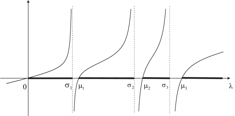
Fig. 2. The graph of the function $\lambda\mathcal{F}(\lambda)$ (for $m=3$).

Let us consider the equation $\lambda\mathcal{F}(\lambda)=a$, where $a\in[0,\infty)$. One the one hand it is equivalent to the equation $\left(\prod\limits_{j=1}^{m}(\sigma_{j}-\lambda)\right)^{-1}P_{m+1}(\lambda)=0$, where $P_{m+1}$ is a polynomial of the degree $m+1$, and therefore in $\mathbb{C}$ this equation at most $m+1$ roots. On the other hand on $[0,\infty)$ the equation $\lambda\mathcal{F}(\lambda)=a$ has exactly $m+1$ roots (see Fig. 2). Thus the set $\{\lambda\in\mathbb{C}:\lambda\mathcal{F}(\lambda)\geq 0\}$ belong to $[0,\infty)$.

We conclude that $\lambda\in\sigma(\mathcal{A}^{0})\setminus\bigcup\limits_{j=1}^{m}\left\{\sigma_{j}\right\}$ iff $\lambda\in[0,\infty)\setminus\left(\bigcup\limits_{j=1}^{m}[\sigma_{j},\mu_{j})\right)$. Since $\sigma(\mathcal{A}^{0})$ is a closed set then the points $\sigma_{j}$, $j=\overline{1,m}$ also belong to $\sigma(\mathcal{A}^{0})$. This completes the proof of equality (1.16).

5. Proof of Hausdorff convergence

This section is a main part of the proof: we show that the set $\sigma(\mathcal{A}^{\varepsilon})$ converges in the Hausdorff sense to the set $\sigma(\mathcal{A}^{0})$ as ${\varepsilon}\to 0$, that is the following conditions (A_H) and (B_H) hold:

$$\text{if }\lambda^{\varepsilon}\in\sigma(\mathcal{A}^{\varepsilon})\text{ and }\lim\limits_{{\varepsilon}\to 0}\lambda^{\varepsilon}=\lambda\text{ then }\lambda\in\sigma(\mathcal{A}^{0})$$ (A_H)

$$\text{for any }\lambda\in\sigma(\mathcal{A}^{0})\text{ there exists }\lambda^{\varepsilon}\in\sigma(\mathcal{A}^{\varepsilon})\text{ such that }\lim\limits_{{\varepsilon}\to 0}\lambda^{\varepsilon}=\lambda$$ (B_H)

5.1. Proof of condition (A_H)

Let $\lambda^{\varepsilon}\in\sigma(\mathcal{A}^{\varepsilon})$, $\lim\limits_{{\varepsilon}\to 0}\lambda^{\varepsilon}=\lambda$. We have to prove that $\lambda\in\sigma(\mathcal{A}^{0})$.

If $\lambda\in\bigcup\limits_{j=1}^{m}\left\{\sigma_{j}\right\}$ then (A_H) holds true since $\bigcup\limits_{j=1}^{m}\left\{\sigma_{j}\right\}\subset\sigma(\mathcal{A}^{0})$. Therefore we focus on the case $\lambda\notin\bigcup\limits_{j=1}^{m}\left\{\sigma_{j}\right\}$.

We consider the sequence ${\varepsilon}_{N}\subset{\varepsilon}$, where ${\varepsilon}_{N}={1\over N}$, $N=1,2,3$… For convenience we preserve the same notation ${\varepsilon}$ having in mind the sequence ${\varepsilon}_{N}$.

Taking into account Remark 2.1 we conclude that there exists $\theta^{\varepsilon}\in\mathbb{T}^{n}$ such that $\lambda^{\varepsilon}\in\sigma(\mathcal{A}^{\theta^{\varepsilon},{\varepsilon}}_{{{{Y}}}})$. We extract a subsequence (still denoted by ${\varepsilon}$) such that $\theta^{\varepsilon}\underset{{\varepsilon}\to 0}{\to}\theta\in\mathbb{T}^{n}$.

Let $u^{\varepsilon}\in\mathrm{dom}(\mathcal{A}^{\theta^{\varepsilon},{\varepsilon}}_{{{{Y}}}})$ be the eigenfunction corresponding to $\lambda^{\varepsilon}$ and such that

$$\|u^{\varepsilon}\|_{L_{2,b^{\varepsilon}}({{{Y}}})}=1\text{ (and therefore }\eta^{\varepsilon}_{{{{Y}}}}[u^{\varepsilon}]=\lambda^{\varepsilon})$$ (5.1)

We introduce the operator $\Pi^{\varepsilon}:H^{1}(F_{Y}^{\varepsilon})\to H^{1}({{{Y}}})$ such that for each $u\in H^{1}(F_{Y}^{\varepsilon})$:

$$\begin{matrix}\Pi^{\varepsilon}u(x)=u(x)\ \text{ for }\ x\in F_{{{Y}}}^{\varepsilon}\\ \|\Pi^{\varepsilon}u\|_{H^{1}({{{Y}}})}\leq C\|u\|_{H^{1}(F_{{Y}}^{\varepsilon})}\end{matrix}$$ (5.2)

It is known (see e.g. [3, 18]) that such an operator exists.

Also we introduce the operators $\Pi_{j}^{\varepsilon}:L_{2}(\cup_{i\in\mathcal{I}^{\varepsilon}}B_{ij}^{\varepsilon})\to L_{2}({{{Y}}})$ ($j=1,\dots,m$) by the formula

$$i\in\mathcal{I}^{\varepsilon},\ x\in{{{Y}}}_{i}^{\varepsilon}:\ \Pi_{j}^{\varepsilon}u(x)=\langle u\rangle_{B_{ij}^{\varepsilon}}$$

(recall that $\overline{{{{Y}}}}=\bigcup\limits_{i\in\mathcal{I}^{\varepsilon}}\overline{{{{Y}}}_{i}^{\varepsilon}}$). Using the Cauchy inequality we obtain

$$\|\Pi_{j}^{\varepsilon}u\|_{L_{2}({{{Y}}})}\leq C\|u\|_{L_{2}(\cup_{i\in\mathcal{I}^{\varepsilon}}B_{ij}^{\varepsilon})}$$ (5.3)

It follows from (5.1)-(5.3) and the embedding theorem that a subsequence (still denoted by ${\varepsilon}$), $u\in H^{1}({{{Y}}})$ and $u_{j}\in L_{2}({{{Y}}})$ ($j=1,\dots,m$) exist such that

$$\Pi^{\varepsilon}u^{\varepsilon}\underset{{\varepsilon}\to 0}{\to}u\text{ weakly in }H^{1}({{{Y}}})\text{ and strongly in }L_{2}({{{Y}}})$$

$$\Pi_{j}^{\varepsilon}u^{\varepsilon}\underset{{\varepsilon}\to 0}{\to}u_{j}\text{ weakly in }L_{2}({{{Y}}})\quad(j=1,\dots,m)$$

Moreover due to the trace theorem

$$\Pi^{\varepsilon}u^{\varepsilon}\underset{{\varepsilon}\to 0}{\to}u\text{ strongly in }L_{2}(\partial{{{Y}}})$$ (5.4)

and therefore $u$ belong to $H^{1}_{\theta}({{{Y}}})$, i.e.

$$\forall k=\overline{1,n}:\quad u(x+e_{k})=\theta_{k}u(x),\text{ for }x=\underset{{}^{\overset{\qquad\quad\uparrow}{\qquad\quad k\text{-th place}}\qquad}}{(x_{1},x_{2},\dots,0,\dots,x_{n})}$$ (5.5)

We denote by $\widehat{\mathcal{A}}_{Y}^{\theta}$ the operator which is defined by the operation $\widehat{\mathcal{A}}_{Y}^{\theta}u=-\displaystyle\sum\limits_{k,l=1}^{n}\widehat{a}^{kl}{\partial^{2}u\over\partial x_{k}\partial x_{l}}$ and the definitional domain $\mathrm{dom}(\widehat{\mathcal{A}}_{Y}^{\theta})$ consisting of functions belonging to $H^{2}({Y})$ and satisfying $\theta$-periodic boundary conditions, i.e.

$$\forall k=\overline{1,n}:\quad\begin{cases}u(x+e_{k})=\theta_{k}u(x),\\ \displaystyle\sum\limits_{l=1}^{n}\widehat{a}^{kl}{\partial u\over\partial x_{l}}(x+e_{k})=\theta_{k}\sum\limits_{l=1}^{n}\widehat{a}^{kl}{\partial u\over\partial x_{l}}(x),\end{cases}\text{ for }x=\underset{{}^{\overset{\qquad\quad\uparrow}{\qquad\quad k\text{-th place}}\qquad}}{(x_{1},x_{2},\dots,0,\dots,x_{n})}$$

It is clear that $\sigma(\widehat{\mathcal{A}}_{Y}^{\theta})\subset[0,\infty)$.

Lemma 5.1.

One has

$$u\in\mathrm{dom}(\widehat{\mathcal{A}}_{Y}^{\theta})\text{ and }\widehat{\mathcal{A}}_{Y}^{\theta}u=\lambda\mathcal{F}(\lambda)u$$ (5.6)

Proof.

One has the following integral equality:

$$\int\limits_{{{{Y}}}}\bigg{(}a^{\varepsilon}(x)\big{(}\nabla u^{\varepsilon}(x),\nabla\mathbf{w}^{\varepsilon}(x)\big{)}-\lambda^{\varepsilon}b^{\varepsilon}(x)u^{\varepsilon}(x)\mathbf{w}^{\varepsilon}(x)\bigg{)}dx=0,\quad\forall\mathbf{w}^{\varepsilon}\in H^{1}_{\overline{\theta^{\varepsilon}}}({{{Y}}})$$ (5.7)

In order to prove (5.6) we plug into (5.7) a function $\mathbf{w}^{\varepsilon}$ of special type and then pass to the limit as ${\varepsilon}\to 0$.

We introduce some additional notations. Let $v_{k}\in C^{2}(F)$ ($k=1,\dots,n$) be a function that solves the problem (1.10) in $F$. We denote by $\widehat{v}_{k}$ the function that belongs to $C^{2}(Y)$ and coincides with $v_{k}$ in $F$ (such a function exists, see e.g. [19]). Then we extend $\widehat{v}_{k}$ by periodicity to the whole $\mathbb{R}^{n}$ preserving the same notation for the extended function. Using a standard regularity theory one can easily prove that $\widehat{v}_{k}\in C^{2}(\mathbb{R}^{n})$. We set

$$v_{k}^{{\varepsilon}}(x)={\varepsilon}\widehat{v}_{k}(x{\varepsilon}^{-1})$$

Let $\mathbf{v}_{ij}^{\varepsilon}\in C^{2,{\varepsilon}}(D_{ij}^{\varepsilon})$ ($i\in\mathbb{Z}^{n},\ j=1,\dots,m$) be the function which is defined in $D_{ij}^{\varepsilon}$ by formula (3.10), $\mathrm{supp}(\mathbf{v}_{ij}^{\varepsilon})\subset D_{ij}^{\varepsilon}$. We redefine it by zero in $\mathbb{R}^{n}\setminus D_{ij}^{\varepsilon}$. Recall that $\mathbf{v}_{ij}^{\varepsilon}$ was constructed in Lemma 3.4 as an approximation for the eigenfunction ${v}_{ij}^{\varepsilon}$ of the operator $\mathcal{A}_{D_{ij}^{\varepsilon}}^{D,{\varepsilon}}$ which corresponds to the first eigenvalue $\lambda_{1}^{D,{\varepsilon}}(D_{ij}^{\varepsilon})$ and satisfies (3.9).

Let $\varphi:\mathbb{R}\to\mathbb{R}$ be a twice-continuously differentiable function such that $\varphi(\rho)=1$ as $\rho\leq 1/2$ and $\varphi(\rho)=0$ as $\rho\geq 1$. We set

$$\varphi_{i}^{\varepsilon}(x)=1-\sum\limits_{j=1}^{m}\varphi\left({|x-x_{ij}^{\varepsilon}|-(r^{\varepsilon}-d^{\varepsilon})\over d^{\varepsilon}}\right),\ x\in\mathbb{R}^{n}$$

Its clear that

$$\begin{matrix}\varphi^{\varepsilon}_{i}(x)=0\text{ for }x\in\bigcup\limits_{j=1}^{m}B_{ij}^{\varepsilon},\quad\varphi^{\varepsilon}_{i}(x)=1\text{ for }x\in\mathbb{R}^{n}\setminus\left(\bigcup\limits_{j=1}^{m}(\overline{G_{ij}^{\varepsilon}\cup B_{ij}^{\varepsilon}})\right)\\ |D^{\alpha}\varphi_{i}^{\varepsilon}|<C{\varepsilon}^{-\alpha\gamma}\ (|\alpha|=0,1,2,\dots)\text{ in }\bigcup\limits_{j=1}^{m}G_{ij}^{\varepsilon}\end{matrix}$$ (5.8)

We cover $\mathbb{R}^{n}$ by the cubes

$$\widetilde{{{{Y}}}}_{i}^{{\varepsilon}}=\left\{x\in\mathbb{R}^{n}:i{\varepsilon}<x_{k}<(i+1){\varepsilon}+{\varepsilon}^{3/2}\right\},\ i\in\mathbb{Z}^{n}$$

Let $\left\{\psi_{i}^{\varepsilon}(x)\right\}_{i\in\mathbb{Z}^{n}}$ be a partition of unity associated with this covering, that is

$$\psi_{i}^{\varepsilon}(x)\in C^{2}(\mathbb{R}^{n}),\quad 0\leq\psi^{\varepsilon}_{i}(x)\leq 1,\quad\sum\limits_{i\in\mathbb{Z}^{n}}\psi^{\varepsilon}_{i}(x)=1,\quad\psi_{i}^{\varepsilon}(x)=1\text{ if }x\in\widetilde{{{{Y}}}}_{i}^{{\varepsilon}}\setminus\bigcup\limits_{l\not=i}\widetilde{{{{Y}}}}_{l}^{{\varepsilon}},\quad\psi_{i}^{\varepsilon}(x)=0\text{ if }x\notin\widetilde{{{{Y}}}}_{i}^{{\varepsilon}}$$

Moreover, analyzing a standard procedure of the construction of the partition of unity (see e.g. [20]) we can easily construct the partition of unity satisfying the following additional conditions

$$\forall i\in\mathbb{Z}^{n},\forall x\in\mathbb{R}^{n}:\ \psi_{i}^{\varepsilon}(x)=\psi^{\varepsilon}_{0}(x+i{\varepsilon})$$ (5.9)

$$D^{\alpha}\psi^{\varepsilon}_{0}(x)<\displaystyle{C{\varepsilon}^{-{3\alpha/2}}}\ (\alpha=0,1,2)\text{ for }x\in\widetilde{Y}_{0}\cap\left(\bigcup\limits_{l\not=0}\widetilde{Y}_{l}\right)$$ (5.10)

We consider the function $w^{\varepsilon}$ of the following form:

$$w^{\varepsilon}(x)=\sum\limits_{i\in\mathbb{Z}^{n}}\psi^{\varepsilon}_{i}(x)\left(g^{\varepsilon}_{i}(x)+h^{\varepsilon}_{i}(x)\right)$$ (5.11)

where

$$\displaystyle g_{i}^{\varepsilon}(x)=g(x^{i,{\varepsilon}})+\varphi_{i}^{\varepsilon}(x)\left(\sum\limits_{k=1}^{n}{\partial g\over\partial x_{k}}(x^{i,{\varepsilon}})\big{(}x_{k}-x_{k}^{i,{\varepsilon}}-v_{k}^{\varepsilon}(x)\big{)}+\right.$$

$$\displaystyle\quad\quad\left.+{1\over 2}\sum\limits_{k,l=1}^{n}{\partial^{2}g\over\partial x_{k}\partial x_{l}}(x^{i,{\varepsilon}})\big{(}x_{k}-x_{k}^{i,{\varepsilon}}-v_{k}^{\varepsilon}(x)\big{)}\big{(}x_{l}-x_{l}^{i,{\varepsilon}}-v_{l}^{\varepsilon}(x)\big{)}\right)$$ (5.12)

$$h_{i}^{\varepsilon}(x)=\sum\limits_{j=1}^{m}\big{(}h_{j}(x_{ij}^{\varepsilon})-g(x_{ij}^{\varepsilon})\big{)}\mathbf{v}_{ij}^{\varepsilon}$$ (5.13)

Here $x^{i,{\varepsilon}}$ is the center of ${Y}_{i}^{\varepsilon}$, $g(x)$, $h_{j}(x)$ are arbitrary functions from $C^{2}(\mathbb{R}^{n})$ satisfying

$$\forall x\in\mathbb{R}^{n},\ \forall i=(i_{1},\dots,i_{n})\in\mathbb{Z}^{n}:\ \begin{cases}g(x+i)=\overline{\theta_{1}^{i_{1}}}\cdot\ldots\cdot\overline{\theta_{n}^{i_{n}}}g(x)\\ h_{j}(x+i)=\overline{\theta_{1}^{i_{1}}}\cdot\ldots\cdot\overline{\theta_{n}^{i_{n}}}h_{j}(x),\ j=1,\dots,m\end{cases}$$ (5.14)

Remark that $\displaystyle{\partial g_{i}^{\varepsilon}\over\partial n}=0$ on $\partial G_{ij}^{\varepsilon}$. Taking this into account we conclude that ${w}^{\varepsilon}(x)$ belongs to $C^{2,{\varepsilon}}(\mathbb{R}^{n})$ and in view of (5.9), (5.14) and the periodicity of $v^{{\varepsilon}}_{k}$ we get

$$\forall x\in\mathbb{R}^{n},\ \forall i\in\mathbb{Z}^{n}:\ w^{\varepsilon}(x+i)=\overline{\theta_{1}^{i_{1}}}\cdot\ldots\cdot\overline{\theta_{n}^{i_{n}}}w^{\varepsilon}(x)$$

We also introduce the notations

$$g^{\varepsilon}=\sum\limits_{i\in\mathbb{Z}^{n}}\psi^{\varepsilon}_{i}(x)g^{\varepsilon}_{i}(x),\quad h^{\varepsilon}=\sum\limits_{i\in\mathbb{Z}^{n}}\psi^{\varepsilon}_{i}(x)h^{\varepsilon}_{i}(x)$$

The function $w^{\varepsilon}$ belong to $H^{1}_{\overline{\theta}}({{{Y}}})$. In order to obtain the function from $H^{1}_{\overline{\theta^{\varepsilon}}}({{{Y}}})$ we modify $w^{\varepsilon}$ multiplying it by the function which is very close to $1$ in ${Y}$ as ${\varepsilon}\to 0$. Namely, we define the function $\mathbf{1}^{\varepsilon}\in C^{\infty}(\mathbb{R}^{n})$ by the following recurrent formulae:

$$\mathbf{1}^{\varepsilon}(x_{1},\dots,x_{n})=A_{n}(x_{1},\dots,x_{n-1})x_{n}+B_{n}(x_{1},\dots,x_{n-1}),$$

$$\alpha=2,\dots,n:\ \begin{cases}B_{\alpha}(x_{1},\dots,x_{\alpha-1})=A_{\alpha-1}(x_{1},\dots,x_{\alpha-2})x_{\alpha-1}+B_{\alpha-1}(x_{1},\dots,x_{\alpha-2}),\\ A_{\alpha}(x_{1},\dots,x_{\alpha-1})=\big{(}{\overline{\theta_{\alpha}^{\varepsilon}}}/{{\overline{\theta_{\alpha}}}}-1\big{)}B_{\alpha}(x_{1},\dots,x_{\alpha-1}),\end{cases}$$

$$B_{1}=1,\ A_{1}={\overline{\theta_{1}^{\varepsilon}}}/{\overline{\theta_{1}}}-1.$$

It is easy to see that

$$\begin{matrix}\max\limits_{x\in\overline{{{{Y}}}}}\left|\mathbf{1}^{\varepsilon}(x)-1\right|+\max\limits_{x\in\overline{{{{Y}}}}}\left|\nabla\mathbf{1}^{\varepsilon}(x)\right|\underset{{\varepsilon}\to 0}{\to}0\\ \mathbf{1}^{\varepsilon}\in H^{1}_{\overline{\theta^{\varepsilon}}/\overline{\theta}}({{{Y}}})\text{, where }\overline{\theta^{\varepsilon}}/\overline{\theta}:=(\overline{\theta_{1}^{\varepsilon}}/\overline{\theta_{1}},\dots,\overline{\theta_{n}^{\varepsilon}}/\overline{\theta_{n}})\end{matrix}$$ (5.15)

Finally we set

$$\mathbf{w}^{\varepsilon}(x)=w^{\varepsilon}(x)+(\mathbf{1}^{\varepsilon}(x)-1)w^{\varepsilon}(x)$$

It is clear that $\mathbf{w}^{\varepsilon}\in H^{1}_{\overline{\theta^{\varepsilon}}}({{{Y}}})$.

Substituting $\mathbf{w}^{\varepsilon}$ into (5.7) and integrating by parts we obtain

$$\int\limits_{{{{Y}}}}\bigg{(}u^{\varepsilon}\mathcal{A}^{\varepsilon}w^{\varepsilon}-\lambda^{\varepsilon}u^{\varepsilon}w^{\varepsilon}\bigg{)}b^{\varepsilon}dx+\\ +\int\limits_{\partial{{{Y}}}}u^{\varepsilon}{\partial w^{\varepsilon}\over\partial n}ds+\int\limits_{{{{Y}}}}{\bigg{(}a^{\varepsilon}\big{(}\nabla u^{\varepsilon},\nabla((\mathbf{1}^{\varepsilon}-1)w^{\varepsilon})\big{)}-\lambda^{\varepsilon}b^{\varepsilon}u^{\varepsilon}(\mathbf{1}^{\varepsilon}-1)w^{\varepsilon}\bigg{)}dx}=0$$ (5.16)

Further we will prove that the second and the third integrals in (5.16) tend to zero as ${\varepsilon}\to 0$. Now we focus on the first integral in (5.16). Using Lemma 3.3 and taking into account (5.1), (5.8) we obtain the estimates

$$\|u^{\varepsilon}\|^{2}_{L_{2}(G_{Y}^{\varepsilon})}\leq C{\varepsilon}^{\gamma-1}\sum\limits_{i\in\mathcal{I}^{\varepsilon}}\left(\eta_{G_{ij}^{\varepsilon}}^{\varepsilon}[u^{\varepsilon}]+{\varepsilon}^{2}\eta_{R_{ij}^{\varepsilon}}^{\varepsilon}[u^{\varepsilon}]+\|u^{\varepsilon}\|^{2}_{L_{2}(R_{ij}^{\varepsilon})}\right)\leq C_{1}{\varepsilon}^{\gamma-1}$$ (5.17)

$$\|\mathcal{A}^{\varepsilon}g^{\varepsilon}\|^{2}_{L_{2}(G_{Y}^{\varepsilon})}\leq C{\varepsilon}^{3-\gamma}$$ (5.18)

Since $\mathcal{\mathcal{A}}^{\varepsilon}h^{\varepsilon}=0$ in $G_{ij}^{\varepsilon}$ then in view of (1.3), (5.17), (5.18)

$$\left|(u^{\varepsilon},\mathcal{\mathcal{A}}^{\varepsilon}w^{\varepsilon})_{L_{2,b^{\varepsilon}}(G_{Y}^{\varepsilon})}\right|\leq C{\varepsilon}\underset{{\varepsilon}\to 0}{\to}0$$ (5.19)

Similarly we obtain

$$\lim\limits_{{\varepsilon}\to 0}(u^{\varepsilon},w^{\varepsilon})_{L_{2,b^{\varepsilon}}(G^{\varepsilon}_{{{Y}}})}=0$$ (5.20)

We denote

$$\widetilde{F}_{i}^{\varepsilon}=\left\{x\in F_{i}^{\varepsilon}:i{\varepsilon}+{\varepsilon}^{3/2}<x_{k}<(i+1){\varepsilon}\right\},\ \widetilde{F}_{Y}^{\varepsilon}=\bigcup\limits_{i\in\mathcal{I}^{\varepsilon}}\widetilde{F}_{i}^{\varepsilon}$$

It is clear that $\widetilde{F}_{i}^{\varepsilon}=F_{i}^{\varepsilon}\setminus\left(\bigcup\limits_{l\not=i}\widetilde{Y}_{l}^{\varepsilon}\right)$.

Firstly we estimate $g^{\varepsilon}$ in $F_{Y}^{\varepsilon}\setminus\widetilde{F}_{Y}^{\varepsilon}$. We represent $g^{\varepsilon}$ in $F_{Y}^{\varepsilon}\setminus\widetilde{F}_{Y}^{\varepsilon}$ in the form

$$g^{\varepsilon}(x)=\sum\limits_{i\in\mathbb{Z}^{n}}\psi_{i}(x)\left[\left(g^{i,{\varepsilon}}+\sum\limits_{k=1}^{n}g_{,k}^{i,{\varepsilon}}\big{(}x_{k}-x^{i,{\varepsilon}}_{k}\big{)}+{1\over 2}\sum\limits_{k,l=1}^{n}g^{i,{\varepsilon}}_{,kl}\big{(}x_{k}-x^{i,{\varepsilon}}_{k}\big{)}\big{(}x_{l}-x^{i,{\varepsilon}}_{l}\big{)}-g(x)\right)-\right.\\ \left.-\sum\limits_{k=1}^{n}\left(g^{i,{\varepsilon}}_{,k}+\sum\limits_{l=1}^{n}g^{i,{\varepsilon}}_{,kl}\big{(}x_{l}-x^{i,{\varepsilon}}_{l}\big{)}-g_{,k}(x)\right)v_{k}^{\varepsilon}(x)+{1\over 2}\sum\limits_{k,l=1}(g^{i,{\varepsilon}}_{,kl}-g_{,kl}(x))v_{k}^{\varepsilon}(x)v_{l}^{\varepsilon}(x)\right]+\\ +g(x)-\sum\limits_{k=1}^{n}g_{,k}(x)v_{k}^{\varepsilon}(x)+{1\over 2}\sum\limits_{k,l=1}^{n}g_{,kl}(x)v_{k}^{\varepsilon}(x)v_{l}^{\varepsilon}(x)$$ (5.21)

Here $g^{i,{\varepsilon}}=g(x^{i,{\varepsilon}})$, $\displaystyle g_{,k}(x)={\partial g\over\partial x_{k}}(x)$, $g_{,k}^{i,{\varepsilon}}=g^{\varepsilon}_{,k}(x^{i,{\varepsilon}})$, $\displaystyle g_{,kl}(x)={\partial^{2}g\over\partial x_{k}\partial x_{l}}(x)$, $g_{,kl}^{i,{\varepsilon}}=g^{\varepsilon}_{,kl}(x^{i,{\varepsilon}})$. It follows from (5.10), (5.21) that $|\Delta g^{\varepsilon}(x)|<C$ for $x\in F_{Y}^{\varepsilon}\setminus\widetilde{F}_{Y}^{\varepsilon}$. Since $\mathrm{dist}\left(\bigcup\limits_{j=1}^{m}D_{ij}^{\varepsilon},\partial Y_{i}^{\varepsilon}\right)\geq\kappa{\varepsilon}$ then $h^{\varepsilon}=0$ in $F_{Y}^{\varepsilon}\setminus\widetilde{F}_{Y}^{\varepsilon}$ when ${\varepsilon}$ is small enough and therefore

$$\left|(u^{\varepsilon},\mathcal{\mathcal{A}}^{\varepsilon}w^{\varepsilon})_{L_{2,b^{\varepsilon}}(F_{Y}^{\varepsilon}\setminus\widetilde{F}_{Y}^{\varepsilon})}\right|\leq C\|\Delta g^{\varepsilon}\|_{L_{2}(F_{Y}^{\varepsilon}\setminus\widetilde{F}_{Y}^{\varepsilon})}\leq C_{1}\sqrt{|F_{Y}^{\varepsilon}\setminus\widetilde{F}_{Y}^{\varepsilon}|}\leq C_{2}{\varepsilon}^{1/4}$$ (5.22)

Similarly we obtain

$$\lim\limits_{{\varepsilon}\to 0}(u^{\varepsilon},w^{\varepsilon})_{L_{2,b^{\varepsilon}}(F_{Y}^{\varepsilon}\setminus\widetilde{F}_{Y}^{\varepsilon})}=0$$ (5.23)

Let us study $g^{\varepsilon}$ and $h^{\varepsilon}$ in $\widetilde{F}^{\varepsilon}$. It is clear that

$$\Delta g^{\varepsilon}=\sum\limits_{k,l=1}^{n}g^{i,{\varepsilon}}_{,kl}\big{(}\nabla(x_{k}-v^{\varepsilon}_{k}),\nabla(x_{l}-v^{\varepsilon}_{l})\big{)}\text{ for }x\in\widetilde{{F}}_{i}^{\varepsilon}$$ (5.24)

In view of Lemma 3.1 and the Poincaré inequality one has the following estimate:

$$\left\|u^{\varepsilon}-\langle u^{\varepsilon}\rangle_{\widetilde{F}_{i}^{\varepsilon}}\right\|^{2}_{L_{2}(\widetilde{F}_{i}^{\varepsilon})}+{\varepsilon}^{n}\left|\langle\Pi^{\varepsilon}u^{\varepsilon}\rangle_{{Y}_{i}^{\varepsilon}}-\langle u^{\varepsilon}\rangle_{\widetilde{F}_{i}^{\varepsilon}}\right|^{2}+\left\|\Pi^{\varepsilon}u^{\varepsilon}-\langle\Pi^{\varepsilon}u^{\varepsilon}\rangle_{{Y}_{i}^{\varepsilon}}\right\|_{L_{2}({{Y}_{i}^{\varepsilon}})}^{2}\leq C{\varepsilon}^{2}\left\|\nabla\Pi^{\varepsilon}u^{\varepsilon}\right\|_{L_{2}({Y}_{i}^{\varepsilon})}^{2}$$ (5.25)

Using (5.24), (5.25) and the Poincaré inequality we get

$$(u^{\varepsilon},\mathcal{A^{\varepsilon}}w^{\varepsilon})_{L_{2,b^{\varepsilon}}(\widetilde{F}_{Y}^{\varepsilon})}=-\sum\limits_{k,l=1}^{n}\left[\left(\int\limits_{F}\big{(}\nabla(x_{k}-v_{k}),\nabla(x_{l}-v_{l})\big{)}dx\right){\varepsilon}^{n}\sum\limits_{i\in\mathcal{I}^{\varepsilon}}g^{i,{\varepsilon}}_{,kl}\langle\Pi^{\varepsilon}u^{\varepsilon}\rangle_{{Y}_{i}^{\varepsilon}}\right]+o(1)=\\ =-\sum\limits_{k,l=1}^{n}\widehat{a}^{kl}|F|\int\limits_{{{{Y}}}}u^{\varepsilon}{\partial^{2}g\over\partial x_{k}\partial x_{l}}dx+o(1)\underset{{\varepsilon}\to 0}{\to}-\sum\limits_{k,l=1}^{n}\widehat{a}^{kl}|F|\int\limits_{{{{Y}}}}u{\partial^{2}g\over\partial x_{k}\partial x_{l}}dx$$ (5.26)

In the same way using Lemma 3.2 (for $v^{\varepsilon}=\Pi^{\varepsilon}u^{\varepsilon}$) we obtain

$$(u^{\varepsilon},g^{\varepsilon})_{L_{2,b^{\varepsilon}}(\widetilde{F}^{\varepsilon}_{{{Y}}})}=\sum\limits_{i\in\mathcal{I}^{\varepsilon}}g(x^{i,{\varepsilon}})\langle u^{\varepsilon}\rangle_{F_{i}^{\varepsilon}}|F|{\varepsilon}^{n}+o(1)\underset{{\varepsilon}\to 0}{\to}{|F|}\int\limits_{{Y}}u(x)g(x)dx$$ (5.27)

(here we also use the estimate ${\varepsilon}^{n}\|\langle u^{\varepsilon}\rangle_{\widetilde{F}_{i}^{\varepsilon}}-\langle u^{\varepsilon}\rangle_{F_{i}^{\varepsilon}}\|^{2}\leq C{\varepsilon}^{2}\|\nabla\Pi^{\varepsilon}u^{\varepsilon}\|^{2}_{L_{2}(Y_{i}^{\varepsilon})}$ which follows from Lemma 3.1).

Let us study $h^{\varepsilon}$ in $\widetilde{F}_{{{Y}}}^{\varepsilon}$. Integrating by parts and taking into account the form of the function $\mathbf{v}_{ij}^{\varepsilon}$ (in particular, we have the estimate $\|\mathcal{A}^{\varepsilon}\mathbf{v}_{ij}^{\varepsilon}\|_{L_{2}(Y_{i}^{\varepsilon})}<C{\varepsilon}^{n}$), the Poincaré inequality and Lemma 3.2 we obtain

$$(u^{\varepsilon},\mathcal{A^{\varepsilon}}h^{\varepsilon})_{L_{2,b^{\varepsilon}}(\widetilde{F}^{\varepsilon}_{{{Y}}})}=(u^{\varepsilon},\mathcal{A^{\varepsilon}}h^{\varepsilon})_{L_{2,b^{\varepsilon}}(F^{\varepsilon}_{{{Y}}})}=\sum\limits_{j=1}^{m}\sum\limits_{i\in\mathcal{I}^{\varepsilon}}\langle u^{\varepsilon}\rangle_{F_{i}^{\varepsilon}}\int\limits_{\hat{C}_{ij}^{\varepsilon}}{\partial\mathbf{v}_{ij}^{\varepsilon}\over\partial r}\left(h_{j}(x_{ij}^{\varepsilon})-g(x_{ij}^{\varepsilon})\right)ds+\\ +\sum\limits_{i\in\mathcal{I}^{\varepsilon}}\left(u^{\varepsilon}-\langle u^{\varepsilon}\rangle_{F_{i}^{\varepsilon}},\mathcal{A}^{\varepsilon}h_{i}^{\varepsilon}\right)_{L_{2,b^{\varepsilon}}(F_{i}^{\varepsilon})}=\sum\limits_{j=1}^{m}a_{j}\left|\partial{B}_{j}\right|\sum\limits_{i\in\mathcal{I}^{\varepsilon}}\langle u^{\varepsilon}\rangle_{F_{i}^{\varepsilon}}\left(g(x_{ij}^{\varepsilon})-h_{j}(x_{ij}^{\varepsilon})\right){\varepsilon}^{n}+o(1)\underset{{\varepsilon}\to 0}{\to}\\ \underset{{\varepsilon}\to 0}{\to}\sum\limits_{j=1}^{m}a_{j}\left|\partial{B}_{j}\right|\int\limits_{{{{Y}}}}u(x)\left(g(x)-h_{j}(x)\right)dx$$ (5.28)

(here $r=|x-x_{ij}^{\varepsilon}|$). In the same way we get

$$\lim\limits_{{\varepsilon}\to 0}(u^{\varepsilon},h^{\varepsilon})_{L_{2,b^{\varepsilon}}(\widetilde{F}^{\varepsilon}_{{{Y}}})}=0$$ (5.29)

Let us study $h^{\varepsilon}$ in $B_{{{Y}}}^{\varepsilon}$ ($g^{\varepsilon}=0$ in $B_{{{Y}}}^{\varepsilon}$). Integrating by parts and using the Poincaré inequality we obtain

$$(u^{\varepsilon},\mathcal{A^{\varepsilon}}h^{\varepsilon})_{L_{2,b^{\varepsilon}}(B^{\varepsilon}_{{{Y}}})}=-\sum\limits_{j=1}^{m}\sum\limits_{i\in\mathcal{I}^{\varepsilon}}\langle u^{\varepsilon}\rangle_{B_{ij}^{\varepsilon}}\int\limits_{\check{C}_{ij}^{\varepsilon}}{\partial\mathbf{v}_{ij}^{\varepsilon}\over\partial r}\left(h_{j}(x_{ij}^{\varepsilon})-g(x_{ij}^{\varepsilon})\right)ds+o(1)=\\ =\sum\limits_{j=1}^{m}a_{j}\left|\partial{B}_{j}\right|\int\limits_{Y}\Pi_{j}^{\varepsilon}u^{\varepsilon}(x)(h_{j}(x)-g(x))dx+o(1)\underset{{\varepsilon}\to 0}{\to}\sum\limits_{j=1}^{m}a_{j}\left|\partial{B}_{j}\right|\int\limits_{{{{Y}}}}u_{j}(x)\left(h_{j}(x)-g(x)\right)dx$$ (5.30)

In the same way we get

$$\lim\limits_{{\varepsilon}\to 0}(u^{\varepsilon},h^{\varepsilon})_{L_{2,b^{\varepsilon}}(B^{\varepsilon}_{{{Y}}})}=\sum\limits_{j=1}^{m}|{B}_{j}|b_{j}\int\limits_{\Omega}u_{j}(x)h_{j}(x)dx$$ (5.31)

Finally, let us estimate the remaining integrals in (5.16). One can easily obtain that

$$\eta_{Y}^{\varepsilon}[w^{\varepsilon}]+\|w^{\varepsilon}\|^{2}_{L_{2,b^{\varepsilon}}({Y})}<C$$

and therefore in view of (5.15)

$$\lim\limits_{{\varepsilon}\to 0}\int\limits_{Y}\bigg{(}a^{\varepsilon}\big{(}\nabla u^{\varepsilon},\nabla((\mathbf{1}^{\varepsilon}-1)w^{\varepsilon})\big{)}-\lambda^{\varepsilon}b^{\varepsilon}u^{\varepsilon}(\mathbf{1}^{\varepsilon}-1)w^{\varepsilon}\bigg{)}dx=0$$ (5.32)

It is easy to see that the function $p^{\varepsilon}=\left.\displaystyle{\partial w^{\varepsilon}\over\partial n}\right|_{\partial{Y}}$ is bounded in $L_{2}(\partial{Y})$ uniformly in ${\varepsilon}$ and therefore there is a subsequence (still denoted by ${\varepsilon}$) and $p\in L_{2}(\partial{Y})$ such that

$$p^{\varepsilon}\underset{{\varepsilon}\to 0}{\to}p\text{ weakly in }L_{2}(\partial{Y})$$ (5.33)

Moreover it is clear that $\forall k=\overline{1,n}$: $p^{\varepsilon}(x+e_{k})=-\overline{\theta_{k}^{\varepsilon}}p^{\varepsilon}(x)$ for $x=\underset{{}^{\overset{\qquad\quad\uparrow}{\qquad\quad k\text{-th place}}\qquad}}{(x_{1},x_{2},\dots,0,\dots,x_{n})}$. Therefore

$$\forall k=\overline{1,n}:\ \quad p(x+e_{k})=-\overline{\theta_{k}}p(x)\text{ for }x=\underset{{}^{\overset{\qquad\quad\uparrow}{\qquad\quad k\text{-th place}}\qquad}}{(x_{1},x_{2},\dots,0,\dots,x_{n})}$$ (5.34)

Taking into account (5.4), (5.5), (5.33), (5.34) we get

$$\lim\limits_{{\varepsilon}\to 0}\int\limits_{\partial{{{Y}}}}u^{\varepsilon}{\partial w^{\varepsilon}\over\partial n}ds=\int\limits_{\partial{Y}}up\ ds=0$$ (5.35)

Then taking into account (5.19), (5.20), (5.22), (5.23), (5.26)-(5.32), (5.35) we pass to the limit in (5.16) and obtain the equality

$$\int\limits_{{Y}}\left(-u(x)|F|\sum\limits_{k,l=1}^{n}\widehat{a}^{kl}{\partial^{2}g\over\partial x_{k}\partial x_{l}}(x)-\lambda|F|u(x)g(x)+\sum\limits_{j=1}^{m}\bigg{(}a_{j}|\partial B_{j}|\big{(}g(x)-h_{j}(x)\big{)}u(x)\right.+\\ \left.+a_{j}|\partial B_{j}|\big{(}h_{j}(x)-g(x)\big{)}u_{j}(x)-\lambda|{B}_{j}|b_{j}u_{j}(x)h_{j}(x)\bigg{)}\right)dx=0$$ (5.36)

Recall that $g,h_{j}\in C^{2}(\mathbb{R}^{n})$ are arbitrary functions satisfying (5.14).

Plugging $g=0$, $h_{j}=0$ for $j\not=k$ into (5.36) and taking into account the equality $|\partial B_{j}|={|B_{j}|nr^{-1}}$ we get

$$u_{k}={\sigma_{k}\over\sigma_{k}-\lambda}u,\quad k\in\{1,\dots,m\}$$ (5.37)

Then setting $h_{j}=0$ for all $j=1,\dots,m$, integrating by parts and taking into account (5.37) we get

$$\int\limits_{{Y}}\left(\sum\limits_{k,l=1}^{n}\widehat{a}^{kl}{\partial u\over\partial x_{k}}{\partial g\over\partial x_{l}}-\lambda\mathcal{F}(\lambda)ug\right)dx=0$$ (5.38)

where the function $\mathcal{F}(\lambda)$ is defined by (1.12).

Equality (5.38) is valid for an arbitrary $g$ belonging to $C^{\infty}(\mathbb{R}^{n})$ and satisfying (5.14). It is clear that the set of such functions is dense in $H_{\overline{\theta}}^{1}({Y})$. Therefore equality (5.38) implies (5.6). Lemma 5.1 is proved. ∎

Lemma 5.2.

$u\not=0$.

Proof.

Let us introduce the spherical coordinates $(r,\Theta)$ in $D_{ij}^{\varepsilon}$ and the function $u_{ij}^{\varepsilon}$ by the formula

$$u_{ij}^{\varepsilon}(\rho,\Theta)=\langle u^{\varepsilon}\rangle_{S^{\varepsilon}_{ij}(\rho)},\text{ where }S^{\varepsilon}_{ij}(\rho)=\left\{x\in\mathbb{R}^{n}:\ |x-x_{ij}^{\varepsilon}|=\rho\right\}$$

One has the following Poincaré inequality:

$$\|u^{\varepsilon}-u_{ij}^{\varepsilon}\|^{2}_{L_{2}(S^{\varepsilon}_{ij}(\rho))}\leq C\rho^{2}\|\nabla_{\Theta}u^{\varepsilon}\|^{2}_{L_{2}(S^{\varepsilon}_{ij}(\rho))}\leq C_{1}{\varepsilon}^{2}\|\nabla u^{\varepsilon}\|^{2}_{L_{2}(S^{\varepsilon}_{ij}(\rho))}$$

(here $\nabla_{\Theta}$ is a gradient on $S_{ij}^{\varepsilon}(\rho)$: for example in the case $n=2$ one has $\nabla_{\Theta}u={1\over\rho^{2}}{\partial u\over\partial\theta}$). Integrating it by $\rho$ from $0$ to $r^{\varepsilon}-d^{\varepsilon}$ and summing by $i$ we get

$$\sum\limits_{i\in\mathcal{I}^{\varepsilon}}\|u^{\varepsilon}-u_{ij}^{\varepsilon}\|^{2}_{L_{2}(B^{\varepsilon}_{ij})}\leq C{\varepsilon}^{2}\|\nabla u^{\varepsilon}\|^{2}_{L_{2}(\bigcup\limits_{i}B_{ij}^{\varepsilon})}\leq C_{1}{\varepsilon}^{2}\lambda^{\varepsilon}$$ (5.39)

We denote ${\mathbf{u}}_{ij}^{\varepsilon}=u_{ij}^{\varepsilon}-\langle u^{\varepsilon}\rangle_{S_{ij}^{\varepsilon}}$. Clearly $\mathbf{u}_{ij}^{\varepsilon}\in\mathrm{dom}(\mathcal{A}_{D_{ij}^{\varepsilon}}^{D,{\varepsilon}})$ and

$$\mathcal{A}_{D_{ij}^{\varepsilon}}^{D,{\varepsilon}}\mathbf{u}_{ij}^{\varepsilon}-\lambda^{\varepsilon}\mathbf{u}_{ij}^{\varepsilon}=\lambda^{\varepsilon}\langle u^{\varepsilon}\rangle_{S_{ij}^{\varepsilon}}$$

Recall that $\lambda\notin\bigcup\limits_{j=1}^{m}\{\sigma_{j}\}$. Then in view of Lemmas 3.4, 3.5 $\lambda^{\varepsilon}\notin\sigma(\mathcal{A}_{D_{ij}^{\varepsilon}}^{D,{\varepsilon}})$ when ${\varepsilon}$ is small enough. Therefore we have the following expansion:

$$\mathbf{u}_{ij}^{\varepsilon}=\sum\limits_{k=1}^{\infty}I^{k}_{ij}({\varepsilon}),\text{ where }I^{k}_{ij}({\varepsilon})={v^{D}_{k}(D_{ij}^{\varepsilon})}{\left(\lambda^{\varepsilon}\langle u^{\varepsilon}\rangle_{S_{ij}^{\varepsilon}},v^{D}_{k}(D_{ij}^{\varepsilon})\right)_{L_{2,b^{\varepsilon}}(D_{ij}^{\varepsilon})}\over\left\|v^{D}_{k}(D_{ij}^{\varepsilon})\right\|_{L_{2,b^{\varepsilon}}(D_{ij}^{\varepsilon})}^{2}\left(\lambda^{D,{\varepsilon}}_{k}(D_{ij}^{\varepsilon})-\lambda^{\varepsilon}\right)}$$ (5.40)

Here $\left\{v^{D}_{k}(D_{ij}^{\varepsilon})\right\}_{k=1}^{m}$ is a system of eigenfunctions of $\mathcal{A}_{D_{ij}^{\varepsilon}}^{D,{\varepsilon}}$ corresponding to $\left\{\lambda^{D,{\varepsilon}}_{k}(D_{ij}^{\varepsilon})\right\}_{k=1}^{m}$ and such that $\left(v^{D}_{k}(D_{ij}^{\varepsilon}),v^{D}_{l}(D_{ij}^{\varepsilon})\right)_{L_{2,b^{\varepsilon}}(D_{ij}^{\varepsilon})}=0$ if $k\not=l$.

Using Lemmas 3.2, 3.5 we get (for $j\in\left\{1,\dots,m\right\}$)

$$\sum\limits_{i\in\mathcal{I}^{\varepsilon}}\left\|\sum\limits_{k=2}^{\infty}I_{ij}^{k}({\varepsilon})\right\|^{2}_{L_{2}(B_{ij}^{\varepsilon})}\leq C\max\limits_{k=\overline{2,\infty}}\left|\lambda^{D,{\varepsilon}}_{k}(D_{ij}^{\varepsilon})-\lambda^{\varepsilon}\right|^{-2}\sum\limits_{i\in\mathcal{I}^{\varepsilon}}\left|\langle u^{\varepsilon}\rangle_{S_{ij}^{\varepsilon}}\right|^{2}{\varepsilon}^{n}\underset{{\varepsilon}\to 0}{\to}0$$ (5.41)

As in Lemma 3.4 we denote $v_{ij}^{\varepsilon}=v^{D}_{1}(D_{ij}^{\varepsilon})$ assuming that $v_{ij}^{\varepsilon}$ is normalized by condition (3.9). Using estimates (3.16), (3.18) and Lemma 3.2 we get

$$\sum\limits_{i\in\mathcal{I}^{\varepsilon}}\left\|I_{ij}^{1}({\varepsilon})\right\|^{2}_{L_{2}(B_{ij}^{\varepsilon})}\sim\sum\limits_{i\in\mathcal{I}^{\varepsilon}}{\lambda^{2}|{B}_{j}|\left|\langle u^{\varepsilon}\rangle_{S_{ij}^{\varepsilon}}\right|^{2}\over(\sigma_{j}-\lambda)^{2}}{\varepsilon}^{n}\sim{\lambda^{2}|{B}_{j}|\|u\|^{2}_{L_{2}({Y})}\over(\sigma_{j}-\lambda)^{2}}$$ (5.42)

as ${\varepsilon}\to 0$. It follows from (5.40)-(5.42) that

$$\lim\limits_{{\varepsilon}\to 0}\sum\limits_{i\in\mathcal{I}^{\varepsilon}}\left\|\mathbf{u}_{ij}^{\varepsilon}\right\|^{2}_{L_{2}(B_{ij}^{\varepsilon})}={\lambda^{2}|B_{j}|\|u\|^{2}_{L_{2}({Y})}\over(\sigma_{j}-\lambda)^{2}}$$ (5.43)

Similarly we obtain

$$\int\limits_{B_{ij}^{\varepsilon}}\mathbf{u}_{ij}^{\varepsilon}dx\sim{\langle u^{\varepsilon}\rangle_{S_{ij}^{\varepsilon}}\lambda|B_{j}|\over\sigma_{j}-\lambda}{\varepsilon}^{n}\text{ as }{\varepsilon}\to 0$$ (5.44)

Using (3.16), (3.18), (5.43), (5.44) and Lemma 3.2 we get

$$\sum\limits_{i\in\mathcal{I}^{\varepsilon}}\left\|u_{ij}^{\varepsilon}\right\|^{2}_{L_{2,b^{\varepsilon}}(B_{ij}^{\varepsilon})}=\sum\limits_{i\in\mathcal{I}^{\varepsilon}}\left(\left\|\mathbf{u}_{ij}^{\varepsilon}\right\|^{2}_{L_{2}(B_{ij}^{\varepsilon})}+2\langle u^{\varepsilon}\rangle_{S_{ij}^{\varepsilon}}\int\limits_{B_{ij}^{\varepsilon}}\mathbf{u}_{ij}^{\varepsilon}(x)dx+\left|\langle u^{\varepsilon}\rangle_{S_{ij}^{\varepsilon}}\right|^{2}\cdot|B_{j}^{\varepsilon}|{\varepsilon}^{n}\right)b_{j}\underset{{\varepsilon}\to 0}{\to}$$

$$\underset{{\varepsilon}\to 0}{\to}\left[{\lambda^{2}|{B}_{j}|\over(\sigma_{j}-\lambda)^{2}}+{2\lambda|{B}_{j}|\over\sigma_{j}-\lambda}+|{B}_{j}|\right]b_{j}\|u\|^{2}_{L_{2}({Y})}=|{B}_{j}|b_{j}\left(\sigma_{j}\over\sigma_{j}-\lambda\right)^{2}\|u\|_{L_{2}({Y})}^{2}$$ (5.45)

Using the Poincaré inequality and Lemma 3.2 one can easily prove that

$$\|u^{\varepsilon}\|^{2}_{L_{2,b^{\varepsilon}}(F_{Y}^{\varepsilon})}=|F|\sum\limits_{i\in\mathcal{I}^{\varepsilon}}\langle u^{\varepsilon}\rangle_{F_{i}^{\varepsilon}}{\varepsilon}^{n}+o(1)\underset{{\varepsilon}\to 0}{\to}|F|\cdot\|u\|^{2}_{L_{2}({Y})}$$ (5.46)

Furthermore in view of Lemma 3.3

$$\lim\limits_{{\varepsilon}\to 0}\|u^{\varepsilon}\|^{2}_{L_{2,b^{\varepsilon}}(G_{Y}^{\varepsilon})}=0$$ (5.47)

Finally taking into account (5.39), (5.45)-(5.47) we obtain

$$1=\|u^{\varepsilon}\|_{L_{2,b^{\varepsilon}}({Y})}^{2}\underset{{\varepsilon}\to 0}{\to}\|u\|^{2}_{L_{2}({Y})}\left[|{F}|+\sum\limits_{j=1}^{m}\left(\sigma_{j}\over\sigma_{j}-\lambda\right)^{2}|B_{j}|b_{j}\right]$$

and therefore $u\not=0$. Lemma 5.2 is proved. ∎

It follows from Lemmas 5.1-5.2 that $\lambda\mathcal{F}(\lambda)$ belong to the spectrum $\sigma(\widehat{\mathcal{A}}^{\theta}_{Y})$ of the operator $\widehat{\mathcal{A}}^{\theta}_{Y}$. Therefore $\lambda\mathcal{F}(\lambda)\in[0,\infty)$ and in view of (4.4) $\lambda\in\sigma(\mathcal{A}^{0})$. Condition (A_H) is proved.

5.2. Proof of condition (B_H)

Let $\lambda\in\sigma(\mathcal{A}^{0})$. Let us prove that there is $\lambda^{\varepsilon}\in\sigma(\mathcal{A}^{\varepsilon})$ such that $\lim\limits_{{\varepsilon}\to 0}\lambda^{\varepsilon}=\lambda$.

We assume the opposite: the subsequence (still denoted by ${\varepsilon}$) and $\delta>0$ exist such that

$$\mathrm{dist}(\lambda,\sigma(\mathcal{A}^{\varepsilon}))>\delta.$$ (5.48)

Since $\lambda\in\sigma(\mathcal{A}^{0})$ then the function $F=\left(\begin{matrix}f\\ f_{1}\\ \dots\\ f_{m}\end{matrix}\right)\in L_{2}(\mathbb{R}^{n})\underset{j=\overline{1,m}}{\oplus}L_{2,{\rho_{j}/\sigma_{j}}}(\mathbb{R}^{n})$ exists such that

$$F\notin\mathrm{im}(\mathcal{A}-\lambda\mathrm{I}),\text{ where }\mathrm{I}\text{ is the identical operator}$$ (5.49)

It follows from (5.48) that $\lambda\in\mathbb{R}\setminus\sigma(\mathcal{A}^{\varepsilon})$. Then $\mathrm{im}(\mathcal{A}^{\varepsilon}-\lambda\mathrm{I})=L_{2,b^{\varepsilon}}(\mathbb{R}^{n})$ and hence for an arbitrary $f^{\varepsilon}\in L_{2,b^{\varepsilon}}(\mathbb{R}^{n})$ there is the unique $u^{\varepsilon}\in\mathrm{dom}(\mathcal{A}^{\varepsilon})$ such that

$$\mathcal{A}^{\varepsilon}u^{\varepsilon}-\lambda u^{\varepsilon}=f^{\varepsilon}$$ (5.50)

We substitute the following $f^{\varepsilon}(x)\in L_{2,b^{\varepsilon}}(\mathbb{R}^{n})$ into (5.50):

$$f^{\varepsilon}(x)=\begin{cases}\langle f\rangle_{Y_{i}^{\varepsilon}},&x\in F_{i}^{\varepsilon},\\ \displaystyle\langle f_{j}\rangle_{Y_{i}^{\varepsilon}},&x\in B_{ij}^{\varepsilon},\\ 0,&x\in\bigcup\limits_{i.j}G_{ij}^{\varepsilon}.\end{cases}$$

It is clear that the norms $\|f^{\varepsilon}\|_{L_{2,b^{\varepsilon}}(\mathbb{R}^{n})}$ are bounded uniformly in ${\varepsilon}$. Then in view of (5.48) $u^{\varepsilon}$ satisfies the inequality

$$\|u^{\varepsilon}\|_{L_{2,b^{\varepsilon}}(\mathbb{R}^{n})}\leq\delta^{-1}{\|f^{\varepsilon}\|_{L_{2,b^{\varepsilon}}(\mathbb{R}^{n})}}\leq C$$

Furthermore

$$\|\nabla u^{\varepsilon}\|^{2}_{L_{2}(\mathbb{R}^{n})}\leq\|f^{\varepsilon}\|_{L_{2,b^{\varepsilon}}(\mathbb{R}^{n})}\cdot\|u^{\varepsilon}\|_{L_{2,b^{\varepsilon}}(\mathbb{R}^{n})}+|\lambda|\cdot\|u^{\varepsilon}\|_{L_{2,b^{\varepsilon}}(\mathbb{R}^{n})}^{2}\leq C$$

Hence a subsequence (still denoted by ${\varepsilon}$) and $u\in H^{1}(\mathbb{R}^{n})$, $u_{j}\in L_{2}(\mathbb{R}^{n})$ such that

$$\Pi^{\varepsilon}u^{\varepsilon}\rightarrow u\text{ weakly in }H^{1}(\mathbb{R}^{n})\text{ and strongly in }L_{2}(G)\text{ for any compact set }G\subset\mathbb{R}^{n}$$

$$\Pi_{j}^{\varepsilon}u^{\varepsilon}\rightarrow u_{j}\text{ weakly in }L_{2}(\mathbb{R}^{n})\ (j=1,\dots,m)$$

where $\Pi^{\varepsilon}$, $\Pi_{j}^{\varepsilon}$ ($j=1,\dots,m$) are the operators introduced above in the proof of condition (A_H).

For an arbitrary ${w}^{\varepsilon}\in\overset{\circ}{C}{}^{\infty}(\mathbb{R}^{n})$ one has the following integral equality:

$$\int\limits_{{{\mathbb{R}^{n}}}}\bigg{(}a^{\varepsilon}(x)\big{(}\nabla u^{\varepsilon}(x),\nabla{w}^{\varepsilon}(x)\big{)}-\lambda^{\varepsilon}b^{\varepsilon}(x)u^{\varepsilon}(x){w}^{\varepsilon}(x)-b^{\varepsilon}(x)f^{\varepsilon}(x){w}^{\varepsilon}(x)\bigg{)}dx=0$$ (5.51)

We substitute into (5.51) the function ${w}^{\varepsilon}$ of the form (5.11)-(5.13), but with $g,h_{j}\in\overset{\circ}{C}{}^{\infty}(\mathbb{R}^{n})$. Making the same calculations as in the proof of condition (A_H) we obtain

$$\int\limits_{\mathbb{R}^{n}}\bigg{[}-u(x)\sum\limits_{k,l=1}^{n}\widehat{a}_{kl}|F|{\partial^{2}g\over\partial x_{k}\partial x_{l}}(x)-\lambda|F|u(x)g(x)-|F|f(x)g(x)+\\ +\sum\limits_{j=1}^{m}\bigg{(}a_{j}|\partial{B}_{j}|\big{(}g(x)-h_{j}(x)\big{)}u(x)+\\ +a_{j}|\partial{B}_{j}|\big{(}h_{j}(x)-g(x)\big{)}u_{j}(x)-\lambda|{B}_{j}|b_{j}u_{j}(x)h_{j}(x)-|{B}_{j}|b_{j}f_{j}(x)h_{j}(x)\bigg{)}\bigg{]}dx=0$$ (5.52)

for an arbitrary $g,h_{j}\in\overset{\circ}{C}{}^{\infty}(\mathbb{R}^{n})$. It follows from (5.52) that

$$U=\left(\begin{matrix}u\\ u_{1}\\ \dots\\ u_{m}\end{matrix}\right)\in\mathrm{dom}(\mathcal{A}^{0})\text{\quad and\quad}\mathcal{A}^{0}U-\lambda U=F$$

We obtain a contradiction with (5.49). Condition (B_H) is proved.

6. End of proof of Theorem 1.1

In general the Hausdorff convergence of $\sigma(\mathcal{A}^{\varepsilon})$ to $\sigma(\mathcal{A}^{0})$ does not imply (1.13)-(1.14). However if we prove that $\sigma(\mathcal{A}^{\varepsilon})$ has at most $m$ gaps in $[0,L]$ when ${\varepsilon}$ is less some ${\varepsilon}_{L}$ then this implication holds true. More precisely the following simple proposition is valid.

Proposition 6.1.

Let $\mathcal{B}^{\varepsilon}=[0,L]\setminus\left(\bigcup\limits_{j=1}^{m^{\varepsilon}}(\alpha_{j}^{\varepsilon},\beta_{j}^{\varepsilon})\right)$, $\mathcal{B}=[0,L]\setminus\left(\bigcup\limits_{j=1}^{m}(\alpha_{j},\beta_{j})\right)$, where $L<\infty$ and

$$0\leq\alpha_{1}^{\varepsilon},\quad\alpha^{\varepsilon}_{j}<\beta^{\varepsilon}_{j}\leq\alpha^{\varepsilon}_{j+1},\ j=\overline{1,m^{\varepsilon}-1},\quad\alpha^{\varepsilon}_{m^{\varepsilon}}\leq L$$

$$0<\alpha_{1},\quad\alpha_{j}<\beta_{j}<\alpha_{j+1},\ j=\overline{1,m-1},\quad\alpha_{m}<L$$

$$m^{\varepsilon}\leq m$$

$$\mathcal{B}^{\varepsilon}\text{ converges to }\mathcal{B}\text{ in the Hausdorff sense as }{\varepsilon}\to 0$$

Then $m^{\varepsilon}=m$ when ${\varepsilon}$ is small enough and

$$\forall j=1,\dots,m:\quad\lim\limits_{{\varepsilon}\to 0}\alpha_{j}^{\varepsilon}=\alpha_{j},\quad\lim\limits_{{\varepsilon}\to 0}\beta_{j}^{\varepsilon}=\beta_{j}$$

We introduce the notation $[a_{k}^{-}({\varepsilon}),a_{k}^{+}({\varepsilon})]:=\bigcup\limits_{\theta\in\mathbb{T}^{n}}\left\{\lambda_{k}^{\theta,{\varepsilon}}({Y}_{0}^{\varepsilon})\right\}$.

Lemma 6.1.

$\lim\limits_{{\varepsilon}\to 0}a_{m+1}^{+}({\varepsilon})=\infty$

Proof.

In the same way as in the proof Lemma 3.5 we obtain the following equality

$$\lim\limits_{{\varepsilon}\to 0}{\varepsilon}^{2}\lambda_{k}^{N,{\varepsilon}}({Y}_{0}^{\varepsilon})=\lambda_{k},\ k=1,2,3...$$ (6.1)

where $\left\{\lambda_{k}\right\}_{k\in\mathbb{N}}$ are the eigenvalues of the operator $\mathbf{A}$ which acts in the space $L_{2}(F)\underset{j=\overline{1,m}}{\oplus}L_{2,b_{j}}({B}_{j})$ and is defined by the operation

$$\mathbf{A}=-\left(\begin{matrix}\Delta^{N}_{F}&0&\dots&0\\ 0&b_{1}^{-1}\Delta^{N}_{{B}_{1}}&\dots&0\\ \vdots&\vdots&\ddots&\vdots\\ 0&0&\dots&b_{m}^{-1}\Delta_{{B}_{m}}^{N}\end{matrix}\right)$$

(here $\Delta^{N}_{F}$ and $\Delta^{N}_{B_{j}}$ are the Neumann Laplacians in $F$ and $B_{j}$). It is clear that $\lambda_{j}=0$ for $j=1,\dots,m+1$ while $\lambda_{m+2}>0$. Then using (6.1) and taking into account (2.3) we get

$$\lim\limits_{{\varepsilon}\to 0}a_{m+2}^{-}({\varepsilon})\geq\lim\limits_{{\varepsilon}\to 0}\lambda_{m+2}^{N}({Y}_{0}^{\varepsilon})=\lambda_{m+2}\lim\limits_{{\varepsilon}\to 0}{\varepsilon}^{-2}=\infty$$

Suppose that there is a subsequence (still denoted by ${\varepsilon}$) such that the numbers $a_{m+1}^{+}({\varepsilon})$ are bounded uniformly in ${\varepsilon}$. Let the numbers $L,L_{1}$ be such that ${\mu_{m}}<L<L_{1}$ and $a_{m+1}^{+}({\varepsilon})<L$. Since $\lim\limits_{{\varepsilon}\to 0}a_{m+2}^{-}({\varepsilon})=\infty$ then $a_{m+2}^{-}({\varepsilon})>L_{1}$ when ${\varepsilon}$ is small enough. Hence $\sigma(\mathcal{A}^{\varepsilon})\cap[L,L_{1}]=\varnothing$ when ${\varepsilon}$ is small enough. We obtain a contradiction with condition (B_H) of the Hausdorff convergence. Thus $\lim\limits_{{\varepsilon}\to 0}a_{m+1}^{+}({\varepsilon})=\infty$. ∎

Lemma 6.1 implies that for an arbitrary $L>0$ the spectrum $\sigma(\mathcal{A}^{\varepsilon})$ has at most $m$ gaps in the interval $[0,L]$ when ${\varepsilon}$ is small enough:

$$\sigma(\mathcal{A}^{\varepsilon})\cap[0,L]=[0,L]\setminus\bigcup\limits_{j=1}^{m^{\varepsilon}}(\sigma_{j}^{\varepsilon},\mu_{j}^{\varepsilon})$$

where $(\sigma_{j}^{\varepsilon},\mu_{j}^{\varepsilon})\subset[0,L]$ are some pairwise disjoint intervals, $m^{\varepsilon}\leq m$. Here the intervals are renumbered in the increasing order.

We have proved that $\sigma(\mathcal{A}^{\varepsilon})$ converges to $[0,\infty)\setminus\left(\bigcup\limits_{j=1}^{m}(\sigma_{j},\mu_{j})\right)$ in the Hausdorff sense as ${\varepsilon}\to 0$. Let $L$ be an arbitrary number such that $L>\mu_{m}$. Then, evidently, $\sigma(\mathcal{A}^{\varepsilon})\cap[0,L]$ converges to $[0,L]\setminus\left(\bigcup\limits_{j=1}^{m}(\sigma_{j},\mu_{j})\right)$ in the Hausdorff sense. By Proposition 6.1 $m^{\varepsilon}=m$ when ${\varepsilon}$ is small enough and

$$\forall j=1,\dots,m:\quad\lim_{{\varepsilon}\to 0}\sigma_{j}^{\varepsilon}=\sigma_{j},\quad\lim_{{\varepsilon}\to 0}\mu_{j}^{\varepsilon}=\mu_{j}$$

Theorem 1.1 is proved.

7. Proof of Theorem 1.2

Substituting $a_{j}$, $b_{j}$ (1.15) into (1.11) we get

$$\sigma_{j}=\alpha_{j}$$

(i.e. the first equality in (0.5) holds) and

$$\rho_{j}=({\beta_{j}-\alpha_{j}})\prod\limits_{i=\overline{1,m}|i\not=j}\displaystyle\left({\beta_{i}-\alpha_{j}\over\alpha_{i}-\alpha_{j}}\right)$$ (7.1)

Recall that $\mu_{j}$ ($j=\overline{1,m}$) are the roots of equation (1.12), therefore in order to prove the equalities $\mu_{j}=\beta_{j}$ ($j=\overline{1,m}$) we have to show that

$$\forall k=1,\dots,m:\ \sum\limits_{j=1}^{m}{\rho_{j}\over\beta_{k}-\alpha_{j}}=1$$ (7.2)

Let us consider (7.2) as a system of $m$ linear algebraic equations ($\rho_{j}$, $j=1,\dots,m$ are unknowns). It is clear that (7.2) follows from the following

Lemma 7.1.

The system (7.2) has the unique solution $\rho_{1},\dots,\rho_{m}$ which is defined by (7.1).

Proof.

We prove the lemma by induction. For $m=1$ its validity is obvious. Suppose that we have proved it for $m=N-1$. Let us prove it for $m=N$.

Multiplying the $k$-th equation in (7.2) ($k=1,\dots,N$) by $\beta_{k}-\alpha_{N}$ and then subtracting the $N$-th equation from the first $N-1$ equations we obtain a new system

$$\forall k=1,\dots,N-1:\ \sum\limits_{j=1}^{N-1}{\hat{\rho}_{j}\over\beta_{k}-\alpha_{j}}=1$$

where the new variables $\hat{\rho}_{j}$, $j=1,\dots,N-1$ are expressed in terms of $\rho_{j}$ by the formula

$$\hat{\rho}_{j}:=\rho_{j}\displaystyle{\alpha_{N}-\alpha_{j}\over\beta_{N}-\alpha_{j}},\ j=1,\dots,N-1$$ (7.3)

Hence $\hat{\rho}_{j}$, $j=\overline{1,N-1}$ satisfy the system (7.2) with $m=N-1$. By the induction

$$\hat{\rho}_{j}=(\beta_{j}-\alpha_{j})\prod\limits_{i=\overline{1,N-1}|i\not=j}\displaystyle\left({\beta_{i}-\alpha_{j}\over\alpha_{i}-\alpha_{j}}\right)$$ (7.4)

It follows from (7.3), (7.4) that $\rho_{j}$ ($j=1,\dots,N-1$) satisfy (7.1) (with $m=N$). The validity of this formula for $\rho_{N}$ follows easily from the symmetry of system (7.2). Lemma 7.1 is proved. ∎

Theorem 1.2 is proved.

References

- [1] G.A. Chechkin, A.L. Piatnitski and A.S. Shamaev, Homogenization. Methods and applications, American Mathematical Society, Providence, 2007.
- [2] D. Cioranescu and P. Donato, An introduction to homogenization, Oxford University Press, Oxford, 1999.
- [3] D. Cioranescu and J. Saint Jean Paulin, Homogenization of Reticulated Structures, Springer, New York, 1999.
- [4] Y. Colin de Verdière, Construction de laplaciens dont une partie finie du spectre est donnee, Ann. Sci. Éc. Norm. Supér. (4) 20(1987), 599-615.
- [5] E.B. Davies and E.M. Harrell, Conformally flat Riemannian metrics, Schrödinger operators, and semiclassical approximation, J. Differ. Equ. 66(1987), 165-188.
- [6] A. Figotin A. and P. Kuchment, Band-gap structure of the spectrum of periodic dielectric and acoustic media. I. Scalar model, SIAM J. Appl. Math. 56(1996), 68-88.
- [7] A. Figotin A. and P. Kuchment, Band-gap structure of the spectrum of periodic dielectric and acoustic media. II. Two-dimensional photonic crystals, SIAM J. Appl. Math. 56(1996), 1561-1620.
- [8] A. Figotin A. and P. Kuchment, Spectral properties of classical waves in high contrast periodic media, SIAM J. Appl. Math. 58(1998), 683-702.
- [9] L. Friedlander, On the density of states of periodic media in large coupling limit, Commun. Partial Differ. Equ. 27(2002), 355-380.
- [10] E.L. Green, Spectral theory of Laplace-Beltrami operators with periodic metrics, J. Differ. Equ. 133(1997), 15-29.
- [11] R. Hempel and K. Lienau, Spectral properties of periodic media in the large coupling limit, Commun. Partial Differ. Eq. 25(2000), 1445-1470.
- [12] R. Hempel and O. Post, Spectral gaps for periodic elliptic operators with high contrast: an overview, Progress in Analysis, Proceedings of the 3rd International ISAAC Congress Berlin 2001 1(2003), 577-587.
- [13] G.A. Iosifyan, O.A. Olejnik and A.S. Shamaev, On the limiting behaviour of the spectrum of a sequence of operators defined on different Hilbert spaces, Russ. Math. Surv. 44(1989), 195-196.
- [14] T. Kato, Perturbation Theory for Linear Operators, Springer-Verlag, Berlin, 1996.
- [15] A. Khrabustovskyi, Asymptotic behaviour of spectrum of Laplace-Beltrami operator on Riemannian manifolds with complex microstructure, Appl. Anal. 87(2008), 1357-1372.
- [16] A. Khrabustovskyi, Periodic Riemannian manifold with preassigned gaps in spectrum of Laplace-Beltrami operator, J. Differ. Equ. 252(2012), 2339-2369.
- [17] P. Kuchment, Floquet Theory for Partial Differential Equations, Birkhauser Verlag, Basel, 1993.
- [18] V.A. Marchenko and E.Ya. Khruslov, Homogenization of Partial Differential Equations, Birkhauser, Boston, 2006.
- [19] V.P. Mikhailov, Partial Differential Equations, Mir Publishers, Moscow, 1978.
- [20] R. Narasimhan, Analysis on Real and Complex Manifolds, Masson et Cie, Paris, 1968.
- [21] L.S. Pankratov and I.D. Chueshov, Averaging of attractors of nonlinear hyperbolic equations with asymptotically degenerate coefficients, Sb. Math. 190(1999), 1325-1352.
- [22] O. Post, Periodic manifolds with spectral gaps, J. Differ. Equ. 187(2003), 23-45.
- [23] M. Reed, B. Simon, Methods of Modern Mathematical Physics IV: Analysis of Operators, Academic Press, New York - San Francisco - London, 1978.
- [24] E. Sanchez-Palencia, Nonhomogeneous Media and Vibration Theory, Springer-Verlag, Berlin, 1980.
- [25] L. Tartar, The General Theory of Homogenization. A Personalized Introduction, Springer, Berlin, 2009.
- [26] V.V. Zhikov, S.M. Kozlov and O.A. Oleinik, Homogenization of Differential Operators and Integral Functionals, Springer, New York, 1994.
- [27] V.V. Zhikov, On gaps in the spectrum of some elliptic operators in divergent form with periodic coefficients, St. Petersb. Math. J. 16(2005), 773-790.