Quantizations on the circle and coherent states

Abstract

We present a possible construction of coherent states on the unit circle as configuration space. Our approach is based on Borel quantizations on $S^{1}$ including the Aharonov-Bohm type quantum description. The coherent states are constructed by Perelomov’s method as group related coherent states generated by Weyl operators on the quantum phase space $\mathbb{Z}\times S^{1}$. Because of the duality of canonical coordinates and momenta, i.e. the angular variable and the integers, this formulation can also be interpreted as coherent states over an infinite periodic chain. For the construction we use the analogy with our quantization and coherent states over a finite periodic chain where the quantum phase space was $\mathbb{Z}_{M}\times\mathbb{Z}_{M}$. The coherent states constructed in this work are shown to satisfy the resolution of unity. To compare them with canonical coherent states, also some of their further properties are studied demonstrating similarities as well as substantial differences.

,

1 Introduction

Quantum description of a particle on a circle is one of the basic problems tackled in quantum mechanics from its beginnings. The reason is that rotational motion represents integral part of important quantum models of atoms, molecules or atomic nuclei.

Coherent states belong to the most useful tools in many applications of quantum physics [1]. They find numerous applications in quantum optics, quantum field theory, condensed matter physics, atomic physics, etc. There exist various definitions and approaches to the coherent states which depend on author and application [2]. Our main reference is [3] since we base our construction of coherent states on the circle on Perelomov’s idea of group-related coherent states, contrary to the overwhelming opinion that this method is not suitable for this purpose.

The problem of coherent states on the circle was investigated by S. de Bièvre [4], and also by J. A. González and M. A. del Olmo [5]. They used the Weil-Brezin-Zak transform $\mathcal{T}$

$$\mathcal{T}:L^{2}(\mathbb{R})\rightarrow L^{2}(S^{1}\times S^{1\ast})$$ (1)

defined by

$$(\mathcal{T}\psi)(q,k):=\sum_{n=-\infty}^{\infty}e^{iank}\psi(q-na),$$ (2)

$$q\in S^{1}=[0,a),\quad k\in S^{1\ast}=[0,\frac{2\pi}{a}),\quad\psi\in L^{2}(\mathbb{R}).$$

Applying this transform to canonical coherent states on the real line they obtained a family of coherent states on the circle labeled by the the variables of the cylinder $\mathbb{R}\times S^{1}$. It should be noted that a very detailed study of deformation quantization on the cylinder as classical phase space was recently given in [6]. The results confirm that in quantum theory the quantum phase space $\mathbb{Z}\times S^{1}$ is involved, which is central point in this investigation.

A different approach was employed by C. J. Isham and J. R. Klauder [7]. They constructed coherent states on the circle by using representations of the Euclidean group $E(2)$. Being the semi-direct product of groups $\mathbb{R}^{2}$ and $SO(2)$, it involves the action on the angular variable. However, they observed that there does not exist an irreducible representation of $E(2)$ such that the resolution of unity holds. Therefore they considered only reducible representations and extended the method to the case of the $n$-dimensional sphere. Other definitions are based on the Lie algebra of $E(2)$ [8, 9] (see also [10]).

We adopt a general method of quantization on configuration manifolds called Borel quantization [11]. According to [11] inequivalent quantum Borel kinematics on a configuration manifold $M$ are classified by elements of the set

$$H^{2}(M,\mathbb{Z})\times H^{1}(M,U(1)).$$

Since $\mbox{dim}\,S^{1}=1$, this implies that the set of inequivalent Borel quantizations is isomorphic to the set $H^{1}(M,U(1))$ of characters of the first homology group $H_{1}(S^{1})=\mathbb{Z}$ (or equivalently, of the fundamental group $\pi_{1}(S^{1})=\mathbb{Z}$). Distinct characters

$$L^{\theta}:\mathbb{Z}\rightarrow U(1):n\mapsto e^{2\pi i\theta n}$$ (3)

are parametrized by $\theta\in[0,1)$.

In general a family of coherent states consists of vectors $|x\rangle$ of some separable Hilbert space $\mathcal{H}$, labeled by some parameter $x\in\mathcal{X}$. Crucial property common to all families of coherent states is the resolution of unity: there exists a positive measure $d\mu(x)$ on $\mathcal{X}$ such that

$$\int_{\mathcal{X}}|x\rangle\langle x|d\mu(x)=\hat{I},$$ (4)

where $\hat{I}$ is the unit operator. The existence of the resolution of unity (4) has to be verified for each family of coherent states. Then, if verified, the resolution of unity (4) entails the completeness of the set of coherent states, i.e. that the closed linear span of the family of coherent states $\{|x\rangle\ \;|\,x\in\mathcal{X}\}$ is the entire Hilbert space $\mathcal{H}$. This property means that any vector in $\mathcal{H}$ may be represented as a linear superposition of coherent states.

Our approach to the construction of coherent states will use Perelomov’s general definition of group-related coherent states [3], where it is assumed that the label space $\mathcal{X}$ has a group structure:

Let $\mathcal{H}$ be a separable Hilbert space, $G$ be a group, $T(g)$ be an arbitrary representation of group $G$ on the Hilbert space $\mathcal{H}$, and $|0\rangle$ be an arbitrary normalized vector in $\mathcal{H}$. Then the set of states $|g\rangle$ defined by

$$|g\rangle=T(g)|0\rangle,\quad g\in G,$$ (5)

is called the system of coherent states related to representation $T$. The state $|0\rangle$ is called the vacuum state.

Our families of coherent states will be of Perelomov type, generated by projective representations of the group $\mathbb{Z}\times U(1)$ and its universal covering with obvious actions on the quantum phase space $\mathbb{Z}\times S^{1}$. Using basic operators of Borel quantum kinematics we shall construct families of Weyl operators which will act on a fiducial vacuum state. Then we shall verify the resolution unity. Among other properties also the inner products of coherent states will be investigated because we shall try to show that their overlap never vanishes like for canonical coherent states. For close comparison with canonical coherent states also the Heisenberg uncertainty product for our coherent states will be examined.

In section 2 we define quantum position and momentum observables on $S^{1}$. Section 3 is devoted to the construction of coherent states on the circle. Here using the basic operators of Borel quantum kinematics a family of Weyl operators is constructed, acting on a vacuum vector. We follow the method of our paper [12], where coherent states on $\mathbb{Z}_{M}\times\mathbb{Z}_{M}$ were studied. In section 4 some properties of the coherent states are studied. In the first place the resolution of unity is proved. Then in section 5 quantizations on $S^{1}$ corresponding to the Aharonov-Bohm type quantum description are formulated. In this framework the coherent states are constructed in the same way as in section 3 and their properties investigated. They satisfy the resolution of unity, too.

2 Quantization on the circle

Let the configuration space be the unit circle $S^{1}$. According to [11] the Hilbert space of quantum mechanics on $S^{1}$ is $\mathcal{H}=L^{2}(S^{1},d\varphi)$ where $\varphi$ is the angle. The position observables are periodic functions of $\varphi$. The momentum operator is defined using the unitary representation $\hat{V}(\alpha)$ of the group of rotations $U(1)$ of the unit circle,

$$[\hat{V}(\alpha)\psi](\beta)=\psi(\beta-\alpha),\quad\psi\in L^{2}(S^{1},d\varphi),\quad\alpha,\beta\in\mathbb{R},$$ (6)

shifting the argument of periodic functions in $L^{2}(S^{1},d\varphi)$. The momentum operator is then by Stone’s theorem

$$\hat{V}(\alpha)=e^{-i\alpha\hat{P}}\quad\Rightarrow\quad\hat{P}=-i\frac{d}{d\varphi}.$$ (7)

The position operator

$$[\hat{Q}\psi](\varphi)=\varphi\psi(\varphi),$$ (8)

formally satisfies usual commutation relation

$$[\hat{Q},\hat{P}]=i\hat{I},$$ (9)

but it is not well-defined on $\mathcal{H}$. As clearly demonstrated in [9], a satisfactory position observable is not $\hat{Q}$ but the unitary operator $e^{i\hat{Q}}$ used in the next section for the construction of coherent states.

In the Dirac notation the position operator satisfies

$$\hat{Q}=\int_{-\pi}^{\pi}\varphi|{\varphi}\rangle\langle{\varphi}|d\varphi,\quad\mbox{with}\quad\langle{\varphi}|{\varphi^{\prime}}\rangle=\delta(\varphi-\varphi^{\prime}).$$

The position operator $\hat{Q}$ has continuous spectrum $\varphi\in[-\pi,\pi)$ with the corresponding eigenvectors $\{|{\varphi}\rangle\}.$ We take the symmetric interval in order that the vacuum state (16) be symmetric around zero. An arbitrary quantum state $|{\psi}\rangle$ can be expressed in the form

$$|{\psi}\rangle=\int_{-\pi}^{\pi}\psi(\varphi)|{\varphi}\rangle d\varphi,\quad\mbox{where}\quad\psi(\varphi)=\langle{\varphi}|{\psi}\rangle.$$

It is useful to expand the periodic wave function $\psi(\varphi)$ in the Fourier series

$$\psi(\varphi)=\sum_{n\in\mathbb{Z}}a_{n}e^{in\varphi}$$ (10)

with the expansion coefficients

$$a_{n}=\frac{1}{2\pi}\int_{S^{1}}e^{-in\varphi}\psi(\varphi)d\varphi.$$ (11)

3 Construction of coherent states

In order to define coherent states directly by Perelomov’s method [3], we should first construct a family of Weyl operators labeled by elements of the group $\mathbb{Z}\times U(1)$. Second, it is necessary to determine the vacuum vector $|0,0\rangle$. The Weyl system is here defined similarly as in [12],

$$\widehat{W}(m,\alpha)=e^{im\hat{Q}}e^{-i\alpha\hat{P}}=e^{im\hat{Q}}\hat{V}(\alpha),\quad\alpha\in[-\pi,\pi),\;m\in\mathbb{Z}.$$ (12)

The factors do not commute

$$e^{im\hat{Q}}e^{-i\alpha\hat{P}}=e^{im\alpha}e^{-i\alpha\hat{P}}e^{im\hat{Q}},$$ (13)

but the operator $e^{im\hat{Q}}$ is now well defined on $\mathcal{H}$,

$$e^{im\hat{Q}}\psi(\varphi)=e^{im\varphi}\psi(\varphi).$$ (14)

Due to (13), the unitary Weyl operators $\widehat{W}(m,\alpha)$ form a projective representation of the group $\mathbb{Z}\times U(1)$.

The vacuum vector $|0,0\rangle$ will be determined in analogy with canonical coherent states on $L^{2}(\mathbb{R})$. The requirement that the vacuum state be an eigenvector of the annihilation operator with eigenvalue $0$ is transcribed like in [12] in exponential form

$$e^{\hat{Q}+i\hat{P}}|0,0\rangle=|0,0\rangle.$$ (15)

Using the Baker-Campbell-Hausdorff formula the operator $e^{\hat{Q}+i\hat{P}}$ can be separated in the product of operators $e^{\hat{Q}}$ and $e^{i\hat{P}}$. Condition (15) leads to a rather fat Gaussian

$$\langle\varphi|0,0\rangle=\mathcal{A}e^{-\frac{\varphi^{2}}{2}},\quad\varphi\in[-\pi,\pi),$$ (16)

sitting on the ‘origin’ of the circle. Hence the vacuum state is an element of our Hilbert space, $|0,0\rangle\in L^{2}(S^{1},d\varphi)$. At $\varphi=\pm\pi$ it is continuous but its derivative has a small discontinuity ($\approx e^{-5}$). The normalization constant $\mathcal{A}$ is given by

$$\mathcal{A}=\frac{1}{\sqrt{\int_{-\pi}^{\pi}exp(-\varphi^{2})d\varphi}}\doteq 0.751128.$$ (17)

The family of coherent states in $L^{2}(S^{1},d\varphi)$ is now generated by the action of the system of unitary Weyl operators $\widehat{W}(m,\alpha)$ on the vacuum state $|0,0\rangle$:

$$|m,\alpha\rangle:=\widehat{W}(m,\alpha)|0,0\rangle.$$ (18)

The functional form of our coherent states is given by

$$\langle\varphi|m,\alpha\rangle=\mathcal{A}e^{im\varphi}e^{-\frac{(\varphi-\alpha)^{2}}{2}},\quad\varphi\in[-\pi,\pi),$$ (19)

i.e. for $\alpha\neq 0$ they are displaced and phased versions of (16) with a discontinuity at $\varphi=\pm\pi$.

4 Properties of our coherent states in $L^{2}(S^{1},d\varphi)$

In this section we shall examine several properties of our coherent states which are known to hold for canonical coherent states on $L^{2}(\mathbb{R})$ [1, 2, 3]. First we shall prove

Theorem. For coherent states (18) the resolution of unity

$$\sum_{k\in\mathbb{Z}}\int_{S^{1}}|k,\alpha\rangle\langle k,\alpha|d\alpha=c\hat{I},$$ (20)

holds, where $c=2\pi$.

Proof. Let us choose an arbitrary normalized vector $\eta\in L^{2}(S^{1},d\varphi)$. Then the inner product of $|\eta\rangle$ with some coherent state $|k,\alpha\rangle$ can be written in the following integral form:

$$\langle k,\alpha|\eta\rangle=\mathcal{A}\int_{S^{1}}e^{-ik\varphi}e^{-\frac{(\varphi-\alpha)^{2}}{2}}\eta(\varphi)d\varphi.$$ (21)

If we denote the operator on the left-hand side of (20) by $\hat{O}$, then we have

$$[\hat{O}\eta](\omega)=\mathcal{A}^{2}\sum_{k\in\mathbb{Z}}\int_{\mathbf{S}^{1}}e^{ik\omega}e^{-\frac{(\omega-\alpha)^{2}}{2}}[\int_{\mathbf{S}^{1}}e^{-ik\varphi}e^{-\frac{(\varphi-\alpha)^{2}}{2}}\eta(\varphi)d\varphi]d\alpha.$$ (22)

Now the expression in the square brackets is in fact $2\pi$ times the $k$-th expansion coefficient (11) of the Fourier decomposition of the function $\exp(-\frac{(\varphi-\alpha)^{2}}{2})\eta(\varphi)$. Applying (10) we obtain

$$[\hat{O}\eta](\omega)=2\pi\mathcal{A}^{2}\int_{\mathbf{S}^{1}}exp(-(\omega-\alpha)^{2})\eta(\omega)d\alpha=2\pi\eta(\omega),$$ (23)

since the integral in (23) yields the squared norm of the coherent state $|m,\alpha\rangle$. $\Box$

Secondly, inner products (overlaps) of our normalized coherent states will be studied. Here it is necessary to correctly realize the way how the operator $\hat{V}(\alpha)=\exp(-i\alpha\hat{P})$ acts on the Hilbert space $L^{2}(S^{1},d\varphi)$ when the circle $S^{1}$ — the configuration space — is identified with the interval $[-\pi,\pi)$. Then the action of operator $e^{-i\alpha\hat{P}}$ on function $\psi(\varphi)\in L^{2}(S^{1},d\varphi)$ for $\alpha\in[0,\pi)$ has the form:

$$e^{-i\alpha\hat{P}}\psi(\varphi) = \psi(\varphi-\alpha)\quad\mbox{for}\quad\varphi\in[-\pi+\alpha,\pi),$$ (24)

$$e^{-i\alpha\hat{P}}\psi(\varphi) = \psi(\varphi-\alpha+2\pi)\quad\mbox{for}\quad\varphi\in[-\pi,-\pi+\alpha).$$ (25)

For $\alpha\in[-\pi,0)$ we have

$$e^{-i\alpha\hat{P}}\psi(\varphi) = \psi(\varphi-\alpha)\quad\mbox{for}\quad\varphi\in[-\pi,\pi+\alpha),$$ (26)

$$e^{-i\alpha\hat{P}}\psi(\varphi) = \psi(\varphi-\alpha-2\pi)\quad\mbox{for}\quad\varphi\in[\pi+\alpha,\pi).$$ (27)

Note that one has to consider addition modulo $2\pi$ in the argument of function $\psi$. For this reason inner products cannot be calculated simply according to

$$\langle m,\alpha|n,\beta\rangle=\mathcal{A}^{2}\int_{-\pi}^{\pi}e^{-i\varphi(n-m)}e^{-\frac{(\varphi-\alpha)^{2}}{2}}e^{-\frac{(\varphi-\beta)^{2}}{2}}d\varphi.$$ (28)

From now on we shall restrict ourselves only to the cases when $\alpha$ and $\beta$ are non-negative numbers:

$$\alpha\in[0,\pi),\quad\beta\in[0,\pi).$$ (29)

Without loss of generality we may also assume

$$\beta\geq\alpha.$$ (30)

Taking into account (24) — (26), we split the inner product of two coherent states into two terms

$$\langle m,\alpha|n,\beta\rangle=\mathcal{A}^{2}I_{1}(\alpha,\beta,n-m)+\mathcal{A}^{2}I_{2}(\alpha,\beta,n-m),$$ (31)

where

$$I_{1}(\alpha,\beta,n-m):=\int_{\alpha-\pi}^{\beta-\pi}e^{i\varphi(n-m)}e^{-\frac{(\varphi-\alpha)^{2}}{2}}e^{-\frac{(\varphi-\beta+2\pi)^{2}}{2}}d\varphi$$ (32)

and

$$I_{2}(\alpha,\beta,n-m):=\int_{\beta-\pi}^{\pi+\alpha}e^{i\varphi(n-m)}e^{-\frac{(\varphi-\alpha)^{2}}{2}}e^{-\frac{(\varphi-\beta)^{2}}{2}}d\varphi.$$ (33)

The integrals $I_{1}(\alpha,\beta,n-m)$ and $I_{2}(\alpha,\beta,n-m)$ can be expressed in terms of the error function of a complex variable $z$,

$$\mbox{erf}(z):=\frac{2}{\sqrt{\pi}}\int_{\Gamma(z)}e^{-\psi^{2}}d\psi;$$ (34)

here $\Gamma(z)$ denotes an arbitrary continuous path of finite length which connects the origin $0\in\mathbb{C}$ with complex number $z\in\mathbb{C}$. Since the Gauss function is analytic, the definition (34) does not depend on the path $\Gamma(z)$.

The integral $I_{1}(\alpha,\beta,n-m)$, after the substitution

$$\omega=\varphi+\pi-\frac{\alpha+\beta}{2},$$ (35)

takes the form

$$I_{1}(\alpha,\beta,n-m) = e^{-(\frac{\beta-\alpha}{2})^{2}-\pi}e^{(\frac{\alpha+\beta}{2}-\pi)(m-n)}\times$$ (36)

$$\times\int_{\frac{\alpha-\beta}{2}}^{\frac{\beta-\alpha}{2}}e^{i\omega(n-m)}e^{-\omega^{2}}d\omega,$$

which leads to the formula

$$I_{1}(\alpha,\beta,n-m) = (-\frac{\sqrt{\pi}}{2})e^{-(\frac{\beta-\alpha}{2})^{2}-\pi}e^{i(\frac{\alpha+\beta}{2}-\pi)(m-n)}e^{-\frac{(n-m)^{2}}{4}}\times$$

$$\times[\mbox{erf}(\frac{\alpha-\beta}{2}+\frac{i(n-m)}{2})+$$

$$+\mbox{erf}(\frac{\alpha-\beta}{2}-\frac{i(n-m)}{2})].$$

The other integral $I_{2}(\alpha,\beta,n-m)$, after the substitution $\omega=\varphi-\frac{\alpha+\beta}{2}$, yields

$$I_{2}(\alpha,\beta,n-m) = (-\frac{\sqrt{\pi}}{2})e^{-(\frac{\beta-\alpha}{2})^{2}}e^{i(\frac{\alpha+\beta}{2})(m-n))}e^{-\frac{(n-m)^{2}}{4}}\times$$

$$\times[\mbox{erf}(\frac{\alpha-\beta}{2}-\pi+\frac{i(n-m)}{2})+$$

$$+\mbox{erf}(\frac{\alpha-\beta}{2}-\pi-\frac{i(n-m)}{2})].$$

We have to admit that, unfortunately, we do not see any way how to further simplify the above analytic expressions of the integrals $I_{1}(\alpha,\beta,n-m)$ and $I_{2}(\alpha,\beta,n-m)$ to see whether the coherent states are mutually non-orthogonal. However, we have numerically computed absolute values of the inner products for many pairs of coherent states and have plotted the graphs of the absolute value of the inner product for several different values of $n-m$ fixed in each graph. It was apparent — for all plotted cases — that the overlap never vanishes. For convenience of the reader we attach in figures 1–3 the graphs of the absolute value of the overlap as function of parameters $\alpha$ and $\beta$ (parameter $n-m$ is fixed for each graph) confirming this property.

Figure 1: Inner product of coherent states on the circle for $m-n=0$.

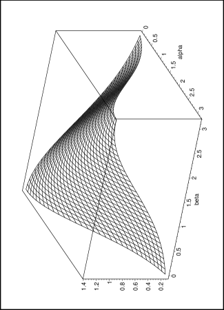
Figure 2: Inner product of coherent states on the circle for $m-n=1$.

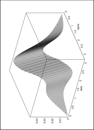
Figure 3: Inner product of coherent states on the circle for $m-n=4$.

The next checked quantities are the expectation values of basic observables in the coherent states $|m,\alpha\rangle$ for $\alpha\geq 0$. Explicitly we have for the position operator

$$\langle m,\alpha|\hat{Q}|m,\alpha\rangle=\mathcal{A}^{2}\int_{-\pi}^{-\pi+\alpha}\varphi e^{-(\varphi-\alpha+2\pi)^{2}}d\varphi+\mathcal{A}^{2}\int_{-\pi+\alpha}^{\pi}\varphi e^{-(\varphi-\alpha)^{2}}d\varphi,$$ (39)

or, using the error function,

$$\langle m,\alpha|\hat{Q}|m,\alpha\rangle=\alpha+q_{1}^{(+)}(\alpha),$$ (40)

where

$$q_{1}^{(+)}(\alpha)=\mathcal{A}^{2}\sqrt{\pi^{3}}(\mbox{erf}(\pi)-\mbox{erf}(\pi-\alpha)).$$ (41)

One observes that the expectation values do not depend on $m$ (this result is obtained also for $\alpha$ negative). Note that the expectation value of position is nonlinear in $\alpha$ for $\alpha\neq 0$. It is clear that for $\alpha=0$ the quasi-Gaussian (16) is symmetric around $\varphi=0$, so the expectation value is an integral of an odd function, evidently equal to zero. However, if $\alpha\neq 0$, the displaced quasi-Gaussian is no more symmetric around $\varphi=0$ and the integration leads to a deviation depending on a difference of error functions (41); maximal deviation is attained for $\alpha\rightarrow\pi$.

Remark [13]. If instead of the expectation values of $\hat{Q}$ expectation values of the unitary position operator $e^{i\hat{Q}}$ are considered in our coherent states, we obtain using (13)

$$\langle m,\alpha|e^{i\hat{Q}}|m,\alpha\rangle=e^{i\alpha}\langle 0,0|e^{i\hat{Q}}|0,0\rangle.$$ (42)

Thus the relative expectation value [9]

$$\frac{\langle m,\alpha|e^{i\hat{Q}}|m,\alpha\rangle}{\langle 0,0|e^{i\hat{Q}}|0,0\rangle}=e^{i\alpha},$$ (43)

yields the exact value of the classical angle, but

$$\langle 0,0|e^{i\hat{Q}}|0,0\rangle\doteq 0.778816$$ (44)

does not lie on the unit circle. Taking into account that $e^{-1/4}\doteq 0.778816$, it turns out that our coherent states yield a very good approximation to formula (3.52) of [9].

The expectation value of the square of position operator in state $|m,\alpha\rangle$ is

$$\langle m,\alpha|\hat{Q}^{2}|m,\alpha\rangle=\mathcal{A}^{2}\int_{-\pi}^{-\pi+\alpha}\varphi^{2}e^{-(\varphi-\alpha+2\pi)^{2}}d\varphi+\mathcal{A}^{2}\int_{-\pi+\alpha}^{\pi}\varphi^{2}e^{-(\varphi-\alpha)^{2}}d\varphi.$$ (45)

The computation gives

$$\langle m,\alpha|\hat{Q}^{2}|m,\alpha\rangle=\alpha^{2}+\frac{1}{2}+q_{2}^{(+)}(\alpha),$$ (46)

where

$$q_{2}^{(+)}(\alpha)=\mathcal{A}^{2}[\pi(e^{-\pi^{2}}-2e^{-(\pi-\alpha)^{2}})+2\sqrt{\pi^{3}}(\pi-\alpha)(\mbox{erf}(\pi)-\mbox{erf}(\pi-\alpha))].$$ (47)

Important among the checked quantities are also the expectation values of the momentum operator in coherent states $|m,\alpha\rangle$. The explicit form

$$\langle m,\alpha|\hat{P}|m,\alpha\rangle = \mathcal{A}^{2}\int_{-\pi}^{-\pi+\alpha}(m+i(\varphi-\alpha+2\pi))e^{-(\varphi-\alpha+2\pi)^{2}}d\varphi$$

$$+ \mathcal{A}^{2}\int_{-\pi+\alpha}^{\pi}(m+i(\varphi-\alpha))e^{-(\varphi-\alpha)^{2}}d\varphi$$

can be simplified into the formula

$$\langle m,\alpha|\hat{P}|m,\alpha\rangle=m,$$ (48)

which could be anticipated by analogy with the canonical coherent states on $L^{2}(\mathbb{R})$.

Finally, the expectation values of the square of momentum operator in coherent states $|m,\alpha\rangle$ are determined by computing the integrals

$$\langle m,\alpha|\hat{P}^{2}|m,\alpha\rangle = \mathcal{A}^{2}\int_{-\pi}^{-\pi+\alpha}[1+(m+i(\varphi-\alpha+2\pi))^{2}]e^{-(\varphi-\alpha+2\pi)^{2}}d\varphi$$ (49)

$$+ \mathcal{A}^{2}\int_{-\pi+\alpha}^{\pi}[1+(m+i(\varphi-\alpha))^{2}]e^{-(\varphi-\alpha)^{2}}d\varphi.$$

The result

$$\langle m,\alpha|\hat{P}^{2}|m,\alpha\rangle=m^{2}+\frac{1}{2}+p_{2}^{(+)},\quad\mbox{where}\quad p_{2}^{(+)}=\mathcal{A}^{2}\pi e^{-\pi^{2}},$$ (50)

does not depend on $\alpha$.

Now these expectation values can be used to form Heisenberg’s uncertainty product for our coherent states. First, the dispersion of the position operator is

$$\Delta_{|m,\alpha\rangle}\hat{Q} = \sqrt{\langle m,\alpha|\hat{Q}^{2}|m,\alpha\rangle-\langle m,\alpha|\hat{Q}|m,\alpha\rangle^{2}}$$ (51)

$$= \sqrt{\frac{1}{2}+q_{2}^{(+)}(\alpha)-2\alpha q_{1}^{(+)}(\alpha)-q_{1}^{(+)}(\alpha)^{2}}.$$

This result is independent of $m$, it depends only on $\alpha$. If both $q_{1}^{(+)}$ and $q_{2}^{(+)}$ were zero, the same value as for canonical coherent states on $L^{2}(\mathbb{R})$ would result, namely $\sqrt{\frac{1}{2}}$. However, the functions $q_{1}^{(+)}$ and $q_{2}^{(+)}$ do not vanish except $q_{1}^{(+)}(0)=0$. Second, the dispersion of the momentum operator in state $|m,\alpha\rangle$ is independent of $m$ and $\alpha$ and different from $\sqrt{\frac{1}{2}}$,

$$\Delta_{|m,\alpha\rangle}\hat{P}=\sqrt{\langle m,\alpha|\hat{P}^{2}|m,\alpha\rangle-\langle m,\alpha|\hat{P}|m,\alpha\rangle^{2}}=\sqrt{\frac{1}{2}+p_{2}^{(+)}}.$$ (52)

So finally the Heisenberg uncertainty product has the form

$$\Delta_{|m,\alpha\rangle}\widehat{Q}\cdot\Delta_{|m,\alpha\rangle}\widehat{P}=\sqrt{\frac{1}{2}+p_{2}^{(\pm)}}\sqrt{\frac{1}{2}+q_{2}^{(\pm)}(\alpha)-2\alpha q_{1}^{(\pm)}(\alpha)-q_{1}^{(\pm)}(\alpha)^{2}},$$ (53)

where superscripts are included also for $\alpha\leq 0$. The results for $\alpha\leq 0$ are given below for completeness:

$$q_{1}^{(-)}(\alpha)=\mathcal{A}^{2}\sqrt{\pi^{3}}(\mbox{erf}(\pi)-\mbox{erf}(\pi+\alpha)),$$

$$q_{2}^{(-)}(\alpha)=\mathcal{A}^{2}[\pi(e^{-\pi^{2}}-2e^{-(\pi-\alpha)^{2}})+2\sqrt{\pi^{3}}(\pi+\alpha)(\mbox{erf}(\pi)-\mbox{erf}(\pi+\alpha))],$$

and

$$p_{2}^{(-)}=\mathcal{A}^{2}\pi\exp(-\pi^{2})=p_{2}^{(+)}.$$

The plot of $\Delta_{|m,\alpha\rangle}\hat{Q}\cdot\Delta_{|m,\alpha\rangle}\hat{P}$ as function of non-negative parameter $\alpha$ is given in figure 4. The graph for $\alpha$ negative is obtained as its even prolongation to $\alpha\leq 0$.

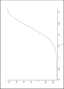
Figure 4: Heisenberg uncertainty product for positive values of $\alpha$.

One can see that $\Delta_{|m,\alpha\rangle}\hat{Q}\cdot\Delta_{|m,\alpha\rangle}\hat{P}$ achieves its minimum for $\alpha=0$, i.e. with

$$q_{1}^{(\pm)}(0)=0,\;q_{2}^{(\pm)}(0)=-\mathcal{A}^{2}\pi e^{-\pi^{2}},\;p_{2}^{(\pm)}=\mathcal{A}^{2}\pi e^{-\pi^{2}}.$$ (54)

Using (53) we get

$$\Delta_{|m,0\rangle}\hat{Q}\cdot\Delta_{|m,0\rangle}\hat{P}=\sqrt{\frac{1}{2}+p_{2}^{(\pm)}}\cdot\sqrt{\frac{1}{2}+q_{2}^{(\pm)}(0)}=\sqrt{\frac{1}{4}-\mathcal{A}^{2}\pi^{2}e^{-2\pi^{2}}}<\frac{1}{2}.$$

Numerical evaluation gives for $\alpha=0$ the actual value $\Delta_{|m,0\rangle}\hat{Q}\cdot\Delta_{|m,0\rangle}\hat{P}\doteq 0.4999999973$, i.e. very slightly below the Heisenberg limit. This circumstance will be discussed in section 6.

5 Quantizations of the Aharonov-Bohm type and coherent states

Let us now describe the quantizations on $S^{1}$ of the Aharonov-Bohm type in the way delineated in [11]. As mentioned in the introduction, inequivalent quantizations are labeled by $\theta\in[0,1)$. They correspond to quantum mechanics of a particle of charge $e$ confined to a circle through which a magnetic flux tube penetrates. The relation of the magnetic flux $\Phi$ to parameter $\theta$ is given by

$$2\pi\theta=\frac{e}{\hbar}\Phi.$$

As before, also in the following we set $\hbar=1$.

The simplest way to obtain the set of quantizations labeled by $\theta$ is to replace the group $U(1)$ by its simply connected universal covering group $\mathbb{R}$ [11]. Action $\sigma$ of $\mathbb{R}$ on $S^{1}$ is natural,

$$\sigma:\mathbb{R}\times S^{1}\rightarrow S^{1}:\;(x,e^{i\varphi})\mapsto e^{i(x+\varphi)},\quad e^{i\varphi}\in S^{1},\;x\in\mathbb{R}.$$ (55)

It is evidently transitive and the stability subgroup is $\mathbb{Z}$. The set of all inequivalent irreducible unitary representations of $\mathbb{Z}$ is labeled by parameter $\theta\in[0,1)$,

$$L^{\theta}:\mathbb{Z}\rightarrow U(1):\;n\mapsto e^{2\pi in\theta}.$$ (56)

These one-dimensional representations classify inequivalent quantum mechanics labeled by parameter $\theta\in[0,1)$. The Hilbert space $\mathcal{H}^{\theta}$ corresponding to parameter $\theta$ contains Borel complex functions $\chi(x)$ on $\mathbb{R}$ with finite norm which are quasi-periodic,

$$\chi(x+2n\pi)=L^{\theta}(n)^{-1}\chi(x)=e^{-2\pi in\theta}\chi(x).$$ (57)

The inner product in $\mathcal{H}^{\theta}$ is

$$(\psi,\chi)_{\theta}=\int_{a}^{a+2\pi}\overline{\psi(x)}\chi(x)dx,\quad a\in\mathbb{R},\quad\psi,\chi\in\mathcal{H}^{\theta}.$$ (58)

The induced unitary representation of the group $\mathbb{R}$ on $\mathcal{H}^{\theta}$ has the simple form

$$[\hat{V}^{\theta}(\alpha)\chi](\beta)=e^{-i\alpha\hat{P}^{\theta}}\chi(\beta)=\chi(\beta-\alpha),\quad\alpha\in\mathbb{R},$$ (59)

hence the momentum operator $\hat{P}^{\theta}$ is simply

$$\hat{P}^{\theta}=-i\frac{d}{dx}.$$ (60)

The position operator on $\mathcal{H}^{\theta}$ is more complicated. It is the multiplication by a saw-shaped function on $\mathbb{R}$,

$$(\hat{Q}\chi)(x)=(x\pmod{2\pi})\chi(x),\quad\chi\in\mathcal{H}^{\theta},$$ (61)

so that function $\hat{Q}\chi(x)$ remains quasi-periodic (57). The momentum operators $\widehat{P}^{\theta}$ have the same form for all $\theta$.

For our calculations it is advantageous to identify the Hilbert spaces $\mathcal{H}^{\theta}$ with the Hilbert space $L^{2}(S^{1},d\varphi)$ of periodic functions $\psi(\varphi)$ via a gauge transformation

$$\mathcal{U}^{\theta}:\mathcal{H}^{\theta}\rightarrow L^{2}(S^{1},d\varphi):\;\chi(\varphi)\mapsto\psi(\varphi)=e^{i\theta\varphi}\chi(\varphi).$$ (62)

The operator $\hat{P}^{\theta}$ on $\mathcal{H}^{\theta}$ is transformed to

$$\widehat{\mathbf{P^{\theta}}}=\mathcal{U}^{\theta}\hat{P}^{\theta}(\mathcal{U}^{\theta})^{-1}=-i\frac{d}{d\varphi}-\theta.$$ (63)

This covariant derivative on $L^{2}(S^{1},d\varphi)$ includes a constant vector potential $A=\Phi/2\pi$ corresponding to the Aharonov-Bohm magnetic flux $\Phi=\int_{S^{1}}Ad\varphi$. The position operator acts by multiplying by independent variable (8).

Let us now define families of coherent states for quantum mechanics labeled by $\theta$. We shall proceed as in the previous chapter working in the Hilbert space $L^{2}(S^{1},d\varphi)$ of periodic functions. It is easy to see that the commutation relation (13) holds in the same form

$$e^{im\hat{Q}}e^{-i\alpha\widehat{\mathbf{P^{\theta}}}}=e^{im\alpha}e^{-i\alpha\widehat{\mathbf{P^{\theta}}}}e^{im\hat{Q}},\quad\alpha\in[-\pi,\pi),\quad m\in\mathbb{Z}.$$ (64)

For the vacuum vector we solve

$$e^{\hat{Q}+i\widehat{\mathbf{P^{\theta}}}}|0,0,\theta\rangle=|0,0,\theta\rangle$$ (65)

and find the vacuum state

$$\langle\varphi|0,0,\theta\rangle=\mathcal{A}_{\theta}e^{-(\varphi-i\theta)^{2}/2},$$ (66)

where the normalization constant

$$\mathcal{A}_{\theta}=\mathcal{A}e^{-\theta^{2}/2}$$

(for $\mathcal{A}$ see (17)). The coherent states are now defined by the action of Weyl operators

$$\widehat{W}^{\theta}(m,\alpha)=e^{im\hat{Q}}e^{-i\alpha\widehat{\mathbf{P^{\theta}}}}$$ (67)

on the vacuum vector and have the following explicit functional form:

$$\langle\varphi|m,\alpha,\phi\rangle = \langle\varphi|\widehat{W}^{\theta}(m,\alpha)|m,\alpha,\theta\rangle=$$ (68)

$$= \mathcal{A}_{\theta}e^{im\varphi}e^{-(\varphi-\alpha-i\theta)^{2}/2},\quad\varphi\in[-\pi,\pi).$$

Now concerning the properties of coherent states for quantum mechanics labeled by parameter $\theta$, we start with

Theorem. For coherent states (68) the resolution of unity

$$\sum_{k\in\mathbb{Z}}\int_{S^{1}}|k,\alpha,\theta\rangle\langle k,\alpha,\theta|d\alpha=c\hat{I},$$ (69)

holds with $c=2\pi$.

Proof. For the proof we take the operator $\hat{O}^{\theta}$ on the left-hand side of (69) and let it act on arbitrary normalized function $\eta\in L^{2}(S^{1},d\varphi)$

$$[\hat{O}^{\theta}\eta](\omega)=$$

$$\mathcal{A}_{\theta}^{2}\sum_{k\in\mathbb{Z}}\int_{S^{1}}e^{ik\omega}e^{-(\omega-\alpha-i\theta)^{2}/2}\cdot[\int_{S^{1}}e^{-ik\varphi}e^{-(\varphi-\alpha+i\theta)^{2}/2}\eta(\varphi)d\varphi]d\alpha.$$ (70)

If we perform similar computation as in (22), we finally obtain

$$[\hat{O}^{\theta}\eta](\omega)=2\pi\mathcal{A}_{\theta}^{2}\eta(\omega)\int_{S^{1}}e^{-(\omega-\alpha-i\theta)^{2}}d\alpha=2\pi\eta(\omega).\Box$$ (71)

Next, we briefly examine the overlaps of the coherent states. We will keep the restrictions (29), (30) on parameters $\alpha$ and $\beta$, and then divide the inner product in two integrals. Proceeding as in (31)

$$\langle m,\alpha,\theta|n,\beta,\theta\rangle=\mathcal{A}_{\theta}^{2}I_{1}(\alpha,\beta,n-m,\theta)+\mathcal{A}_{\theta}^{2}I_{2}(\alpha,\beta,m-n,\theta),$$ (72)

we have

$$I_{1}(\alpha,\beta,n-m,\theta)=\int_{\alpha-\pi}^{\beta-\pi}e^{i\varphi(n-m)}e^{-\frac{(\varphi-\alpha+i\theta)^{2}}{2}}e^{-\frac{(\varphi-\beta+2\pi-i\theta)^{2}}{2}}d\varphi$$ (73)

and

$$I_{2}(\alpha,\beta,n-m,\theta)=\int_{\beta-\pi}^{\pi+\alpha}e^{i\varphi(n-m)}e^{-\frac{(\varphi-\alpha+i\theta)^{2}}{2}}e^{-\frac{(\varphi-\beta-i\theta)^{2}}{2}}d\varphi.$$ (74)

Computation of $I_{1}(\alpha,\beta,n-m,\theta)$ and $I_{2}(\alpha,\beta,n-m,\theta)$ gives us

$$I_{1}(\alpha,\beta,n-m,\theta)=$$

$$e^{\theta^{2}}e^{-i\theta(\beta-\alpha+2\pi)}(-\frac{\sqrt{\pi}}{2})e^{-(\frac{\beta-\alpha}{2})^{2}-\pi}e^{i(\frac{\alpha+\beta}{2}-\pi)(m-n)}e^{-\frac{(n-m)^{2}}{4}}\times$$

$$\times[\mbox{erf}(\frac{\alpha-\beta}{2}+\frac{i(n-m)}{2})+\mbox{erf}(\frac{\alpha-\beta}{2}-\frac{i(n-m)}{2})]$$ (75)

and

$$I_{2}(\alpha,\beta,n-m,\theta)=$$

$$e^{\theta^{2}}e^{-i\theta(\beta-\alpha)}(-\frac{\sqrt{\pi}}{2})e^{-(\frac{\beta-\alpha}{2})^{2}}e^{i(\frac{\alpha+\beta}{2})(m-n))}e^{-\frac{(n-m)^{2}}{4}}\times$$

$$\times[\mbox{erf}(\frac{\alpha-\beta}{2}-\pi+\frac{i(n-m)}{2})+\mbox{erf}(\frac{\alpha-\beta}{2}-\pi-\frac{i(n-m)}{2})].$$ (76)

Comparing these results with (4) and (4), we can write

$$I_{1}(\alpha,\beta,n-m,\theta)=e^{\theta^{2}}e^{-i\theta(\beta-\alpha+2\pi)}I_{1}(\alpha,\beta,n-m)$$ (77)

and

$$I_{2}(\alpha,\beta,n-m,\theta)=e^{\theta^{2}}e^{-i\theta(\beta-\alpha)}I_{2}(\alpha,\beta,n-m).$$ (78)

The inner product for two coherent states is finally

$$\langle m,\alpha,\theta|n,\beta,\theta\rangle=$$

$$=\mathcal{A}^{2}e^{-i\theta(\beta-\alpha+2\pi)}I_{1}(\alpha,\beta,n-m)+\mathcal{A}^{2}e^{-i\theta(\beta-\alpha)}I_{2}(\alpha,\beta,m-n).$$ (79)

The expectation values of position and momentum operators and their squares were also computed. For $\alpha\geq 0$ the correction functions in (41), (47) and (50) are changed to

$$q_{1}^{(+)\theta}(\alpha) = \mathcal{A}_{\theta}^{2}\sqrt{\pi^{3}}(\mbox{erf}(\pi)-\mbox{erf}(\pi-\alpha)),$$

$$q_{2}^{(+)\theta}(\alpha) = \mathcal{A}_{\theta}^{2}[\pi(e^{-\pi^{2}}-2e^{-(\pi-\alpha)^{2}})+2\sqrt{\pi^{3}}(\pi-\alpha)(\mbox{erf}(\pi)-\mbox{erf}(\pi-\alpha))],$$

$$p_{2}^{(+)\theta} = \mathcal{A}_{\theta}^{2}\pi\exp(-\pi^{2}).$$

The Heisenberg uncertainty product for $\alpha\geq 0$ is then

$$\Delta_{|m,\alpha,\theta\rangle}\hat{Q}\cdot\Delta_{|m,\alpha,\theta\rangle}\hat{P}^{\theta}=$$

$$=\sqrt{\frac{1}{2}+p_{2}^{(+)\theta}}\cdot\sqrt{\frac{1}{2}+q_{2}^{(+)\theta}(\alpha)-2\alpha q_{1}^{(+)\theta}(\alpha)-q_{1}^{(+)\theta}(\alpha)^{2}}.$$ (80)

The discussion about possible relevance of the uncertainty product is postponed to the next section.

6 Conclusion

This work was devoted to a construction of coherent states on the circle and investigation of their properties. We used quantizations on the circle with and without an Aharonov-Bohm type flux with parameter $\theta$ related to the magnetic flux through the circle. In these cases we introduced Weyl operators, which were then used to construct group-related coherent states in the sense of Perelomov. If the parameter $\theta$ vanishes, then the results of section 5 fully correspond to the results without magnetic flux given in sections 2–4, as expected.

For the obtained families of coherent states the property of resolution of unity was proved. Also their overlaps and matrix elements were expressed using the analytic error function $\mbox{erf}(z)$. Some results were calculated numerically or evaluated with the help of MATHEMATICA. For instance, the absolute value of the inner product is plotted in figures 1–3 for three choices of the parameters. We have briefly reported on the matter in [14]. On the one hand, we did not dwell on some evident consequences of the resolution of unity like the reproducing kernel property of the overlaps. Also the issue of a Bargmann-Segal representation seems to require a deeper study because of integral values of parameter $m$.

On the other hand, we devoted much effort to compare our coherent states with canonical coherent states which provide wave packets minimizing Heisenberg’s uncertainty relations. For this reason the circle — the configuration space — was identified with the interval $[-\pi,\pi)$. The action of $\hat{Q}$ (or $\hat{Q}^{2}$) considered on $L^{2}(-\pi,\pi)$ is well defined because $\hat{Q}$ is bounded. However, the momentum operator $\hat{P}$ is unbounded. Therefore the Heisenberg uncertainty relation is valid only on a very narrow set of states which belong to a common invariant domain of self-adjoint operators $\hat{Q}$, $\hat{P}$. It is very clearly described e.g. in Chapter 8 of [15] that such a domain exists and the Heisenberg uncertainty relation is valid on it (see also [16] and the references therein).

However, our coherent states do not belong to this domain, in particular because they violate conditions at the ends of the interval $[-\pi,\pi]$. Especially they are not in the domains of operators $\hat{P}^{2}$ and $\hat{P}\hat{Q}$. Therefore, for the sake of evaluating the dispersion $\Delta\hat{P}$ and its comparison with canonical coherent states, we considered $\hat{P}$ and $\hat{P}^{2}$ as formal differential operators. This may explain our results, notably formula (4) showing that Heisenberg’s inequality is violated for coherent states with $\alpha$ close to $0$.

Summarizing, we arrived at limits of similarity between our coherent states and canonical coherent states. In particular we cannot use Heisenberg’s uncertainty theorem which guarantees the well known inequality, because our states do not fulfil assumptions of this theorem. Our coherent states are well defined as elements of the Hilbert space $\mathcal{H}=L^{2}(S^{1},d\varphi)$, but Heisenberg’s theorem requires to essentially narrow down the set of admissible states. Note that Heisenberg’s theorem cannot be applied even to eigenstates of $\hat{P}$ or $\hat{P}^{2}$ since they do not belong to the domain of $\hat{P}\hat{Q}$.

Let us remind that the Aharonov-Bohm type quantizations of [11] were studied by several alternative methods: see e.g. [17] (Feynman’s path integral in non-simply connected spaces), [18] (self-adjoint extensions of the momentum operator) and [19] (non-relativistic current algebras). For a thorough discussion of quantizations on the circle with and without magnetic flux we refer also to the recent article [16].

References

References

[1] Ali S T, Antoine J-P and Gazeau J-P 2000
Coherent States, Wavelets and Their Generalizations
(New York: Springer)
[2]
Klauder J R and Skagerstam B S 1985
Coherent States: Applications in Physics and Mathematical Physics
(Singapore: World Scientific)
[3] Perelomov M A 1986 Generalized Coherent States
and Their Applications (Berlin: Springer)
[4]
de Bièvre S 1989 Coherent states over symplectic homogenous spaces,
J Math Phys30 1401–1407
[5]
González J A and del Olmo M A 1998
Coherent states on the circle
J Phys A: Math Gen31 8841–8857
[6]
González J A del Olmo M A and Tosiek J 2003
Quantum mechanics on the cylinder
J Opt B: Quantum Semiclass Opt5 S306–S315
[7]
Isham C J and Klauder J R 1991 Coherent states for
-dimensional Euclidean groups and their application
J Math Phys32(3) 607–620
[8]
Kowalski K and Rembielinski J 2008
Coherent states for the quantum mechanics on a compact manifold
J Phys A: Math Gen41 (2008) 304021 (12pp)
[9]
Kowalski K, Rembielinski J and Papaloucas L C 1996
Coherent states for the quantum particle on a circle
J Phys A: Math Gen29 4149–4167
[10]
Nieto L M, Atakishiyev N M, Chumakov S M and Wolf K B 1998
Wigner distribution function for Euclidean systems
J Phys A: Math Gen31 3875–3895
[11] Doebner H-D, Šťovíček P and Tolar J
2001 Quantization of kinematics on configuration manifolds
Rev. Math. Phys.13(7) 799–845
[12]
Tolar J and Chadzitaskos G 1997 Quantization on and
coherent states over
J Phys A: Math Gen30 2509–2517
[13] We thank one of the referees for this remark.
[14]
Chadzitaskos G, Luft P and Tolar J 2011
Coherent states on the circle
J Phys A: Conference Series284 012016 (7 pp)
[15]
Blank J, Exner P and Havlíček M 2008
Hilbert Space Operators in Quantum Physics
(AIP Series in Computational and Applied Mathematical Physics)
(New York: Springer & AIP)
[16]
Kastrup H A 2006
Quantization of the canonically conjugate pair angle and orbital
angular momentum
Phys Rev A73 052104 (26 pp)
[17]
Schulman L S 1968
A path integral for spin
Phys Rev176 1558–1569
[18]
Martin C 1976
A mathematical model for the Aharonov-Bohm effect
Lett Math Phys1 155–163
[19] Goldin G A, Menikoff R and Sharp D H 1981
Representations of a local current algebra in
non-simply connected space and the Aharonov-Bohm effect
J Math Phys22 1664–1668