Fusion tilings with infinite local complexity

Abstract.

We propose a formalism for tilings with infinite local complexity (ILC), and especially fusion tilings with ILC. We allow an infinite variety of tile types but require that the space of possible tile types be compact. Examples include solenoids, pinwheel tilings, tilings with fault lines, and tilings with infinitely many tile sizes, shapes, or labels. Special attention is given to tilings where the infinite local complexity comes purely from geometry (shears) or comes purely from combinatorics (labels). We examine spectral properties of the invariant measures and define a new notion of complexity that applies to ILC tilings.

1. Definitions

In the standard theory of tiling dynamical systems, which is motivated in part by the discovery of aperiodic solids, tilings are constructed from a finite number of tile types that can be thought of as atoms. It is usually assumed that these prototiles have only a finite number of possible types of adjacencies and this is called finite local complexity, or FLC. Recently, many interesting tiling models have arisen that do not satisfy this property.

In a tiling with infinite local complexity (ILC), there are infinitely many 2-tile patterns, that is, infinitely many ways for two tiles to meet. Consider an ILC tiling that is made from a finite set of tile types. If we then ‘collar’ the tiles by marking each tile by the pattern of tiles around it, we obtain an equivalent tiling with infinitely many tile types. We therefore allow arbitrarily many tile types from the start, but require that the space of tile types should be compact. In particular, it should only be given the (usual) discrete topology when the set of possible tiles is finite.

1.1. Tiles, labels, patches, tilings, and hulls.

We will construct tilings of Euclidean space $\displaystyle{\mathbb{R}}^{d}$. A tile $\displaystyle t$ is a pair $\displaystyle t=(supp(t),{label}(t))$, where $\displaystyle supp(t)$, the support, is a closed set homeomorphic to a ball in $\displaystyle{\mathbb{R}}^{d}$, and $\displaystyle{label}(t)$ is an element of some compact metric space $\displaystyle{\mathcal{L}}$. We will move tiles around using the action of translation by all elements of $\displaystyle{\mathbb{R}}^{d}$. An element $\displaystyle x\in{\mathbb{R}}^{d}$ acts on a tile $\displaystyle t$ by acting on its support: $\displaystyle t-x=(supp(t)-x,{label}(t))$. Two tiles $\displaystyle t_{1}$ and $\displaystyle t_{2}$ are said to be equivalent if there is an $\displaystyle x\in{\mathbb{R}}^{d}$ such that $\displaystyle t_{1}-x=t_{2}$. In particular, they must have the same label. Equivalent tiles are said to have the same tile type. For convenience we collect one representative of each tile type into a prototile set $\displaystyle{\mathcal{P}}$. This is equivalent to picking a point in the tile, called a control point, that is placed at the origin. If the tiles are convex, then it is often convenient to pick each tile’s control point to be its center of mass.

If a sequence of tile labels converges in $\displaystyle{\mathcal{L}}$ to a limiting label, we require that the supports of the corresponding prototiles converge in the Hausdorff metric to the support of the prototile with the limiting label. This condition constrains both the shapes of the prototiles and the locations of the control points. This is where our paradigm separates from the ‘usual’ tiling theory: not only can there be infinitely many tile types, but those tile types may approximate one another.

The condition also implies that all tiles with a given label are equivalent. Labels serve primarily to distinguish between tile types whose prototiles have identical supports.

Given a fixed prototile set $\displaystyle{\mathcal{P}}$, we can form patches and tilings using copies of tiles from $\displaystyle{\mathcal{P}}$. A $\displaystyle{\mathcal{P}}$-patch (or patch, for short) is a connected union of tiles equivalent to tiles from $\displaystyle{\mathcal{P}}$, whose supports intersect only on their boundaries. A tiling $\displaystyle{\bf T}$ is an infinite patch whose support covers all of $\displaystyle{\mathbb{R}}^{d}$. An equivalent definition of finite local complexity (FLC) is that $\displaystyle{\bf T}$ contains only a finite number of two-tile patches up to translational equivalence.

We make a metric on tiles that will be extended to tilings. The distance between two tiles is $\displaystyle d(t_{1},t_{2})=max\{d_{H}(supp(t_{1}),supp(t_{2})),d_{\mathcal{L}}({label}(t_{1}),{label}(t_{2}))\}$, where $\displaystyle d_{H}$ is Hausdorff distance on subsets of $\displaystyle{\mathbb{R}}^{d}$ and $\displaystyle d_{\mathcal{L}}$ is the metric on $\displaystyle{\mathcal{L}}$. We can extend this to finite patches that have a one-to-one correspondence between their tiles by letting the distance between two patches be the maximum distance between pairs of corresponding tiles. Finally we extend this to tilings by saying that the distance between two tilings is the minimum $\displaystyle\epsilon$ for which the two tilings have patches containing the ball of radius $\displaystyle 1/\epsilon$ around the origin that differ by at most $\displaystyle\epsilon$. If there is no $\displaystyle\epsilon\leq 1$ for which this is true, we simply define the distance between the tilings to be $\displaystyle 1$.

Given a fixed tiling $\displaystyle{\bf T}$, the continuous hull $\displaystyle\Omega_{\bf T}$ of $\displaystyle{\bf T}$ is the closure of the translational orbit of $\displaystyle{\bf T}$:

$$\Omega_{\bf T}=\overline{\{{\bf T}-x\text{ such that }x\in{\mathbb{R}}^{d}\}}$$

More generally, a tiling space $\displaystyle\Omega$ is a closed, translationally invariant set of tilings constructed using some fixed prototile set. In both cases we have a dynamical system $\displaystyle(\Omega,{\mathbb{R}}^{d})$ which we can study from topological or measure-theoretic perspectives.

The tiling space $\displaystyle\Omega$ is necessarily compact. This follows from the compactness of $\displaystyle{\mathcal{P}}$ together with the fact that the possible offsets between the control points of two adjacent tiles lie in a closed and bounded subset of $\displaystyle{\mathbb{R}}^{d}$. Given any sequence of tilings $\displaystyle{\bf T}_{n}\in\Omega$, there is a subsequence whose tiles at the origin converge in both label and position, a subsequence of that for which the tiles touching the “seed” tile converge, a further subsequence for which a second ring of tiles converges, and so on. From Cantor diagonalization we then get a subsequence that converges everywhere. Note that if $\displaystyle{\mathcal{P}}$ were not required to be compact, then $\displaystyle\Omega$ typically would not be compact, either; a sequence of tilings with a non-convergent sequence of tiles at the origin does not have had a convergent subsequence.

1.2. Forms of infinite local complexity

There are a number of standard examples of tilings with ILC, exhibiting different ways that ILC emerges. In some tilings, tiles appear in an infinite number of shapes, or even an infinite number of sizes. In others, the geometry of the tiles is simple, but tiles come with an infinite number of labels. In others, there are only finitely many tile types, but infinitely many ways for two tiles to meet.

Bratteli-Vershik systems [7] are associated with 1-dimensional subshifts (and hence with FLC tilings) and also with non-expansive automorphisms of a Cantor set. These non-expansive automorphisms can be realized as ILC fusion tilings with an infinite tile set.

In the pinwheel tiling [10], all tiles are 1–2–$\displaystyle\sqrt{5}$ right triangles, but the triangles point in infinitely many directions, uniformly distributed on the circle. With respect to translations, that means infinitely many tile types. Versions of the generalized pinwheel [12] exhibit tiles that are similar triangles, pointing in infinitely many directions and having infinitely many different sizes.

ILC tilings can also occur with finite tile sets. One can have shears along a “fault line” where the tiles on one side of the line are offset from the tiles on the other side. For instance, imagine a tiling of $\displaystyle{\mathbb{R}}^{2}$ by two types of tiles, one a rectangle of irrational width $\displaystyle\alpha$ and height 1, and the other a unit square. Imagine that these tiles assemble into alternating rows of unit-width and width-$\displaystyle\alpha$ tiles. There will be infinitely many offsets between adjacent tiles along each boundary between rows. This behavior occurs frequently in tilings generated by substitutions and generalized substitutions when the linear stretching factor is not a Pisot number [2, 4, 5, 8, 12].

1.3. Outline

In Section 2 we review the formalism of fusion for FLC tilings and adapt the definitions to the ILC setting. Most well-known examples of ILC tilings are fusion tilings, and much can be said about them. Many of the results of [6] carry over, only with finite-dimensional vectors replaced by measures and with matrices replaced by maps of measures. In Section 3 we consider dynamical properties such as minimality and expansivity. Some well-known results concerning expansivity do not carry over to the ILC setting, and we define strong expansivity to account for the differences. In Section 4 we address the measure theory of ILC tilings, especially ILC fusion tilings. In Section 5 we adapt ideas of topological pressure and topological entropy to define a complexity function for ILC tilings. We also relate this complexity to expansivity. Finally, in Section 6 we survey the landscape of ILC tilings, defining different classes of ILC tilings, and seeing how various examples fit into the landscape. In the Appendix we present several examples in detail.

Acknowledgments. We thank Ian Putnam for hospitality and many helpful discussions. We thank the Banff International Research Station and the participants of the 2011 Banff workshop on Aperiodic Order. The work of L.S.  is partially supported by NSF grant DMS-1101326.

2. Compact fusion rules and fusion tilings

In previous work [6] we defined fusion rules for tilings with finite local complexity, and now we adapt this definition to handle compact tiling spaces. Given two $\displaystyle{\mathcal{P}}$-patches $\displaystyle P_{1}$ and $\displaystyle P_{2}$ and two translations $\displaystyle x_{1},x_{2}\in{\mathbb{R}}^{d}$, if the union $\displaystyle P_{1}-x_{1}\cup P_{2}-x_{2}$ forms a $\displaystyle{\mathcal{P}}$-patch, and if $\displaystyle P_{1}-x_{1}$ and $\displaystyle P_{2}-x_{2}$ have no tiles in common, we call the union of $\displaystyle P_{1}-x_{1}$ and $\displaystyle P_{2}-x_{2}$ the fusion of $\displaystyle P_{1}$ to $\displaystyle P_{2}$. Patch fusion is simply a version of concatenation for geometric objects.

Intuitively, a fusion tiling develops according to an atomic model: we have atoms, and those atoms group themselves into molecules, which group together into larger and larger structures. Let $\displaystyle{\mathcal{P}}_{0}={\mathcal{P}}$ be our prototile set, our “atoms”. $\displaystyle{\mathcal{P}}$ is labeled by a compact set $\displaystyle{\mathcal{L}}_{0}$. The first set of “molecules” they form is a set $\displaystyle{\mathcal{P}}_{1}$ of finite $\displaystyle{\mathcal{P}}_{0}$-patches. To each element of $\displaystyle{\mathcal{P}}_{1}$ we associate a (distinct) label from a compact set $\displaystyle{\mathcal{L}}_{1}$. We use the notation $\displaystyle{\mathcal{P}}_{1}=\{P_{1}(c)|c\in{\mathcal{L}}_{1}\}$, where for each $\displaystyle c\in{\mathcal{L}}_{1}$ the patch $\displaystyle P_{1}(c)$ is a finite fusion of elements of $\displaystyle{\mathcal{P}}_{0}$.

Similarly, $\displaystyle{\mathcal{P}}_{2}$ is a set of finite patches, indexed by a compact label set $\displaystyle{\mathcal{L}}_{2}$, that are fusions of the patches in $\displaystyle{\mathcal{P}}_{1}$, and we write $\displaystyle{\mathcal{P}}_{2}=\{P_{2}(c)|c\in{\mathcal{L}}_{2}\}$. We continue in this fashion, constructing $\displaystyle{\mathcal{P}}_{n}$ as a set of finite patches that are fusions of elements of $\displaystyle{\mathcal{P}}_{n-1}$, labeled by some compact set $\displaystyle{\mathcal{L}}_{n}$. While the elements of $\displaystyle{\mathcal{P}}_{n}$ are technically $\displaystyle{\mathcal{P}}$-patches, we can also think of them as $\displaystyle{\mathcal{P}}_{k}$-patches for any $\displaystyle k\leq n$ by considering the elements of $\displaystyle{\mathcal{P}}_{k}$ as prototiles. At each stage we assume that the locations of the patches are chosen such that $\displaystyle{\mathcal{P}}_{k}$ is homeomorphic to $\displaystyle{\mathcal{L}}_{k}$. We require consistency between the metrics on the supertile sets in a way we will describe in section 2.1.

The elements of $\displaystyle{\mathcal{P}}_{n}$ are called $\displaystyle n$-supertiles. We collect them together into an atlas of patches we call our fusion rule:

$${\mathcal{R}}=\left\{{\mathcal{P}}_{n},n\geq 0\right\}=\left\{P_{n}(c)\,\,|\,\,n\in{\mathbb{N}}\text{ and }c\in{\mathcal{L}}_{n}\right\}.$$

We say that a finite patch is admitted by $\displaystyle{\mathcal{R}}$ if it can be arbitrarily well approximated by subsets of elements of $\displaystyle{\mathcal{R}}$. If it actually appears inside $\displaystyle P_{n}(c)$ for some $\displaystyle n$ and $\displaystyle c\in{\mathcal{L}}_{n}$, we say it is literally admitted and if it appears only as the limit of literally admitted patches we say it is admitted in the limit. A tiling $\displaystyle{\bf T}$ of $\displaystyle{\mathbb{R}}^{d}$ is said to be a fusion tiling with fusion rule $\displaystyle{\mathcal{R}}$ if every patch of tiles contained in $\displaystyle{\bf T}$ is admitted by $\displaystyle{\mathcal{R}}$. We denote by $\displaystyle\Omega_{\mathcal{R}}$ the set of all $\displaystyle{\mathcal{R}}$-fusion tilings.

For any $\displaystyle n$ we may consider the related space $\displaystyle\Omega^{(n)}_{\mathcal{R}}$ that consists of the same tilings as $\displaystyle\Omega_{\mathcal{R}}$, except that the prototiles are elements of $\displaystyle{\mathcal{P}}_{n}$ instead of $\displaystyle{\mathcal{P}}_{0}$. That is, we ignore the lowest $\displaystyle n$ levels of the hierarchy. In a fusion tiling, we can break each $\displaystyle n$-supertile into $\displaystyle(n-1)$-supertiles using the subdivision map $\displaystyle\sigma_{n}$, which is a map from $\displaystyle\Omega^{(n)}_{\mathcal{R}}$ to $\displaystyle\Omega^{(n-1)}_{\mathcal{R}}$. It is clear that this subdivision map is always a continuous surjection, but it may not be an injection. If for all $\displaystyle n$ it is, then we call the fusion rule recognizable. Recognizability means that there is a unique way to decompose each tiling as a union of $\displaystyle n$-supertiles.

To avoid trivialities, we assume that each $\displaystyle{\mathcal{P}}_{n}$ consists only of supertiles that actually appear in some tiling in $\displaystyle\Omega^{(n)}_{\mathcal{R}}$. We can always achieve this by shrinking each set $\displaystyle{\mathcal{P}}_{n}$, eliminating those spurious supertiles that do not appear in any tilings. We also assume that each $\displaystyle{\mathcal{P}}_{n}$ is non-empty, which is equivalent to $\displaystyle\Omega_{\mathcal{R}}$ being non-empty.

2.1. Metric on $\displaystyle{\mathcal{L}}_{n}$ and $\displaystyle{\mathcal{P}}_{n}$

Each $\displaystyle{\mathcal{L}}_{n}$ is assumed to be a compact metric space, with a metric compatible with the metric defined on lower levels of the hierarchy. Specifically, if two labels in $\displaystyle{\mathcal{L}}_{n}$ are within $\displaystyle\epsilon$, then the prototiles $\displaystyle P,P^{\prime}\in{\mathcal{P}}_{n}$ that represent them must have constituent $\displaystyle(n-1)$-supertiles that are in one-to-one correspondence, that differ by no more than $\displaystyle\epsilon$ in the Hausdorff metric on their supports, and whose labels differ by no more than $\displaystyle\epsilon$ in $\displaystyle{\mathcal{L}}_{n-1}$.

In most examples we will want the metric on $\displaystyle{\mathcal{L}}_{n}$ to be induced directly from the metric on $\displaystyle{\mathcal{L}}_{n-1}$. That is, for two $\displaystyle n$-supertiles to be considered close if and only if all of their constituent $\displaystyle(n-1)$-supertiles are close, and (by induction) if and only if all of their consitutent tiles are close. However, there are important examples where this is not the case, where two $\displaystyle n$-supertiles with different labels may have identical decompositions into $\displaystyle(n-1)$-supertiles. This can occur naturally when $\displaystyle{\mathcal{L}}_{n}$ contains collaring information, and is essential to a variety of collaring schemes.

Besides being compact metric spaces, the sets $\displaystyle{\mathcal{L}}_{n}$ must admit well-defined $\displaystyle\sigma$-algebras of measurable subsets. We will henceforth assume that these algebras have been specified, and speak freely of measurable subsets of $\displaystyle{\mathcal{L}}_{n}$. Since $\displaystyle{\mathcal{P}}_{n}$ is homeomorphic to $\displaystyle{\mathcal{L}}_{n}$, we can also speak of measurable subsets of $\displaystyle{\mathcal{P}}_{n}$.

2.2. The transition map

A standard construct in both self-similar tiling and substitution sequence theory is the transition matrix, whose $\displaystyle(i,j)$ entry counts how many tiles of type $\displaystyle i$ are found in a substituted tile of type $\displaystyle j$. A similar analysis applies to fusions with FLC [6], where $\displaystyle M_{n,N}(i,j)$ tells how many $\displaystyle n$-supertiles of type $\displaystyle i$ are found in an $\displaystyle N$-supertile of type $\displaystyle j$. These matrices satisfy $\displaystyle M_{n,N}=M_{n,m}M_{m,N}$ for each integer $\displaystyle m$ between $\displaystyle n$ and $\displaystyle N$. Many ergodic properties of a fusion tiling space, such as whether it is uniquely ergodic, reduce to properties of these matrices [6].

An apparent obstacle for fusion rules on non-FLC spaces is that the spaces $\displaystyle{\mathcal{L}}_{n}$ that label $\displaystyle n$-supertiles need not be finite. However, since we require each $\displaystyle n$-supertile to be a finite fusion of $\displaystyle(n-1)$-supertiles, we can still define the transition map $\displaystyle M_{n,N}:{\mathcal{P}}_{n}\times{\mathcal{P}}_{N}\to{\mathbb{Z}}$ by

$$\displaystyle M_{n,N}(P,Q) \displaystyle= \displaystyle\#(P\text{ in }Q)$$

$$\displaystyle:= \displaystyle\text{ the number of }n\text{-supertiles equivalent to }P\text{ in the }N\text{-supertile }Q.$$

Thus the $\displaystyle Q$th ‘column’ $\displaystyle M_{n,N}(*,Q)$ gives the breakdown of $\displaystyle Q$ in terms of the $\displaystyle n$-supertiles that it contains, and will consist of 0’s except in finitely many places. If there is more than one way that the $\displaystyle n$-supertiles can be fused to create $\displaystyle Q$ (that is, if the fusion is not recognizable), we fix a preferred one to use in this and all other computations.

We will use the transition map in three different ways throughout this paper: as defined above, as a measure on $\displaystyle{\mathcal{P}}_{n}$, and as an operator mapping (“pushing forward”) measures on $\displaystyle{\mathcal{P}}_{N}$ to measures on $\displaystyle{\mathcal{P}}_{n}$. We give the details on these three views in subsection 4.4. As in the FLC case, the transition map determines quite a bit about the invariant probability measures on $\displaystyle\Omega_{\mathcal{R}}$.

Example 1.

Pinwheel tilings. In the pinwheel tiling, all tiles are $\displaystyle 1,2,\sqrt{5}$ right triangles, but tilings consist of tiles pointing in infinitely many directions. We call a triangle with vertices at $\displaystyle(-1.5,-.5)$, $\displaystyle(.5,-.5)$ and $\displaystyle(.5,.5)$ right-handed and give it label (R,0), and a triangle with vertices at $\displaystyle(-1.5,.5)$, $\displaystyle(.5,.5)$ and $\displaystyle(.5,-.5)$ is called left-handed and has label (L,0). Our label set $\displaystyle{\mathcal{L}}_{0}$ consists of two circles, and the prototile with label (R,$\displaystyle\theta$) (resp.(L,$\displaystyle\theta$)) is obtained by rotating the (R,0) (resp. (L,0)) prototile counterclockwise around the origin by $\displaystyle\theta$. Two tiles are close in our tile metric if they have the same handedness, if their angles $\displaystyle\theta$ are close, and if their centers are close. This is the same as being close in the Hausdorff metric.

Likewise, $\displaystyle{\mathcal{L}}_{n}$ consists of two circles, with the $\displaystyle(R,\theta)$ $\displaystyle n$-supertile being an expansion by $\displaystyle 5^{n/2}$ of the $\displaystyle(R,\theta)$ tile, and likewise for the $\displaystyle(L,\theta)$ $\displaystyle n$-supertile. Let $\displaystyle\alpha=\tan^{-1}(1/2)$. Each $\displaystyle(R,\theta)$ $\displaystyle n$-supertile is built from five $\displaystyle(n-1)$-supertiles, two of type $\displaystyle(L,\theta+\alpha)$, one of type $\displaystyle(L,\theta+\alpha+\frac{\pi}{2})$, one of type $\displaystyle(R,\theta+\alpha)$ and one of type $\displaystyle(R,\theta+\alpha+\pi)$, arranged as in Figure 1.

Figure 1. The pinwheel fusion rule builds $\displaystyle n$-supertiles from five $\displaystyle(n-1)$-supertiles

Likewise, each $\displaystyle(L,\theta)$ $\displaystyle n$-supertile is built from $\displaystyle(n-1)$-supertiles of type $\displaystyle(R,\theta-\alpha)$, $\displaystyle(R,\theta-\alpha-\frac{\pi}{2})$, $\displaystyle(L,\theta-\alpha)$ and $\displaystyle(L,\theta-\alpha+\pi)$.

To compute the transition map, consider $\displaystyle M_{n,(n+1)}((H,\omega),(R,\theta))$. It equals 1 if $\displaystyle(H,\omega)=(R,\theta+\alpha),(R,\theta+\alpha+\pi)$, or $\displaystyle(L,\theta+\alpha+\pi/2)$, it equals 2 when $\displaystyle(H,\omega)=(L,\theta+\alpha)$, and it equals 0 otherwise. Transition for the $\displaystyle(n+1)$-supertile of type $\displaystyle(L,\theta)$ is similar.

Since this example involves infinite many tile orientations, it necessarily involves infinitely many tile labels. The infinite local complexity has both a combinatorial and a geometrical aspect, but both are consequences of rotational symmetry. We call this rotational infinite local complexity.

Example 2.

Shear infinite local complexity. In our next example, each $\displaystyle{\mathcal{P}}_{n}$ consists of only four supertiles, and the infinite local complexity comes from the geometry of how two tiles can touch. Let $\displaystyle{\mathcal{P}}_{0}=\left\{\raisebox{-11.38092pt}{\includegraphics[width=28.45274pt]{DPVtiles-a.png}},\raisebox{-11.38092pt}{\includegraphics[width=28.45274pt]{DPVtiles-b.png}},\raisebox{-11.38092pt}{\includegraphics[width=17.07182pt]{DPVtiles-c.png}},\raisebox{-11.38092pt}{\includegraphics[width=17.07182pt]{DPVtiles-d.png}}\right\}$, where the long edges are of some fixed length $\displaystyle\alpha$ and the short edges are of length $\displaystyle 1$.

For the $\displaystyle 1$-supertiles we choose $\displaystyle{\mathcal{P}}_{1}=\left\{\raisebox{-22.76228pt}{\includegraphics[width=56.9055pt]{DPVlevel1-a.png}},\raisebox{-22.76228pt}{\includegraphics[width=56.9055pt]{DPVlevel1-b.png}},\raisebox{-22.76228pt}{\includegraphics[width=22.76228pt]{DPVlevel1-c.png}},\raisebox{-22.76228pt}{\includegraphics[width=19.91684pt]{DPVlevel1-d.png}}\right\}.$ It is convenient to think of the four supertiles as being of types $\displaystyle a,b,c,d$, using the notation $\displaystyle{\mathcal{P}}_{1}=\{P_{1}(a),P_{1}(b),P_{1}(c),P_{1}(d)\}$. We construct the $\displaystyle n$-supertiles from the level $\displaystyle(n-1)$-supertiles using the same combinatorics as we did to make the 1-supertiles from the prototiles. For instance, $\displaystyle{\mathcal{P}}_{2}(a)=\raisebox{-71.13188pt}{\includegraphics[width=142.26378pt]{DPVlevel2-asuper}}=\raisebox{-71.13188pt}{\includegraphics[width=142.26378pt]{DPVlevel2-a}}$.

If $\displaystyle\alpha$ is chosen irrational, then fault lines develop. There are countably many 2-tile patterns that are literally admitted and uncountably many that are admitted in the limit. If $\displaystyle\alpha$ is chosen rational, then there are only finitely many ways for two $\displaystyle n$-supertiles to meet, but this number increases with $\displaystyle n$. Either way, the large-scale structure of the tilings is different from that of a self-similar FLC substitution tiling. These differences show up in the spectral theory, cohomology, and complexity. (See [4, 5] and references therein.)

Since at each stage there are only four supertile types, the transition operator $\displaystyle M_{n,n+1}$ is the matrix $\displaystyle\left[\begin{matrix}1&1&1&1\\ 3&0&3&0\\ 3&3&0&0\\ 9&0&0&0\end{matrix}\right]$ and $\displaystyle M_{n,N}$ is the $\displaystyle(N-n)$th power of this matrix.

Example 3.

Combinatorial infinite local complexity. Because its (translational) dynamical system is not expansive, the dyadic solenoid system is not topologically conjugate to a tiling system with finite local complexity. However, it can be expressed as an ILC fusion tiling with infinitely many tile labels. In this example the geometry is trivial and the infinite local complexity is purely combinatorial.

The prototiles are unit length tiles that carry labels $\displaystyle\{A_{0},A_{1},\ldots\}\cup\{A_{\infty}\}$, such that $\displaystyle A_{\infty}=\lim_{n\to\infty}A_{n}$ is the only accumulation point of the label set. We define

$${\mathcal{P}}_{1}=\{A_{1}A_{0},A_{2}A_{0},A_{3}A_{0},...,A_{\infty}A_{0}\},$$

in other words $\displaystyle P_{1}(k)=A_{k}A_{0}$ for $\displaystyle k=1,2,\ldots,\infty$. Similarly we define

$${\mathcal{P}}_{2}=\{P_{1}(2)P_{1}(1),P_{1}(3)P_{1}(1),...,P_{1}(\infty)P_{1}(1)\}.$$

In general, every element of $\displaystyle{\mathcal{P}}_{n+1}$ takes the form $\displaystyle P_{n+1}(k)=P_{n}(k)P_{n}(n)$, for all $\displaystyle k\geq n+1$ including $\displaystyle k=\infty$.

Tilings admitted by this fusion rule have $\displaystyle A_{0}$ in every other spot, $\displaystyle A_{1}$ in every fourth spot, and so on, with each species $\displaystyle A_{k}$ with $\displaystyle k<\infty$ appearing in every $\displaystyle(2^{k+1})$-st spot. In addition, there may be one (and only one) copy of $\displaystyle A_{\infty}$. Since all $\displaystyle A_{n}$ tiles with $\displaystyle n\geq k$ have the same location (mod $\displaystyle 2^{k}$), the location of an arbitrary $\displaystyle A_{n}$ with $\displaystyle n\geq k$ gives a map to $\displaystyle S^{1}={\mathbb{R}}/2^{k}{\mathbb{Z}}$. Taken together, these maps associate a tiling with a point in the dyadic solenoid $\displaystyle\varprojlim({\mathbb{R}}/2^{k}{\mathbb{Z}})$. A discrete version of this construction, mimicking an odometer rather than a solenoid, is called a “Toeplitz flow”. [3]

$\displaystyle M_{n,n+1}(k,l)$ equals $\displaystyle 1$ if $\displaystyle k=n$ or if $\displaystyle k=l$, and otherwise it is 0. For $\displaystyle N>n$ and relevant values of $\displaystyle(k,l)$, $\displaystyle M_{n,N}(k,l)$ equals $\displaystyle 2^{N-k-1}$ if $\displaystyle k<N$, $\displaystyle 1$ if $\displaystyle k=l$, and 0 otherwise.

The complexity and ergodic theory of these examples will be worked out in the Appendix.

2.3. Primitivity and the van Hove property

A fusion rule is said to be primitive if for any positive integer $\displaystyle n$ and any open set $\displaystyle U$ of supertiles in $\displaystyle{\mathcal{P}}_{n}$, there is an $\displaystyle N>n$ such that every element of $\displaystyle{\mathcal{P}}_{N}$ contains an element of $\displaystyle U$. Primitivity means that the space $\displaystyle\Omega_{\mathcal{R}}$ is fairly homogeneous, in that each tiling contains patches arbitrarily close to any particular admissible patch.

A van Hove sequence $\displaystyle\{A_{m}\}$ of subsets of $\displaystyle{\mathbb{R}}^{d}$ consists of sets whose boundaries are increasingly trivial relative to their interiors in a precise sense. For any set $\displaystyle A\in{\mathbb{R}}^{d}$ and $\displaystyle r>0$, let

$$A^{+r}=\{x\in{\mathbb{R}}^{d}:\text{ dist}(x,A)\leq r\},$$

where “dist” denotes Euclidean distance. A sequence of sets $\displaystyle\{A_{n}\}$ of sets in $\displaystyle{\mathbb{R}}^{d}$ is called a van Hove sequence if for any $\displaystyle r\geq 0$

$$\lim_{n\to\infty}\frac{\text{Vol}\left((\partial A_{n})^{+r}\right)}{\text{Vol}(A_{n})}=0,$$

where $\displaystyle\partial A$ is the boundary of $\displaystyle A$ and Vol is Euclidean volume.

Given a fusion rule $\displaystyle{\mathcal{R}}$, we may make a sequence of sets in $\displaystyle{\mathbb{R}}^{d}$ by taking one $\displaystyle n$-supertile for each $\displaystyle n$ and calling its support $\displaystyle A_{n}$. We say $\displaystyle{\mathcal{R}}$ is a van Hove fusion rule if every such sequence is a van Hove sequence. Equivalently, a fusion rule is van Hove if for each $\displaystyle\epsilon>0$ and each $\displaystyle r>0$ there exists an integer $\displaystyle n_{0}$ such that each $\displaystyle n$-supertile $\displaystyle A$, with $\displaystyle n\geq n_{0}$, has $\displaystyle\text{Vol}(\partial A)^{+r}<\epsilon\text{Vol}(A)$.

3. Dynamics of ILC tiling spaces

A compact tiling space $\displaystyle\Omega_{\mathcal{R}}$, by definition, is invariant under translation by elements of $\displaystyle{\mathbb{R}}^{d}$. The action of translation is continuous in the tiling metric and gives rise to a topological dynamical system $\displaystyle(\Omega_{\mathcal{R}},{\mathbb{R}}^{d})$. Tiling dynamical systems have been studied extensively in the FLC case, and in this section we investigate the dynamics of ILC tiling systems in general and in the fusion situation. We show under what circumstances a fusion tiling dynamical system is minimal, and we discuss what expansivity means and introduce the related concept of strong expansivity.

3.1. Minimality

Recall that a topological dynamical system is said to be minimal if every orbit is dense.

Proposition 3.1.

If the fusion rule $\displaystyle{\mathcal{R}}$ is primitive, then the fusion tiling space $\displaystyle(\Omega_{\mathcal{R}},{\mathbb{R}}^{d})$ is minimal. Conversely, if $\displaystyle{\mathcal{R}}$ is recognizable and van Hove but is not primitive, then $\displaystyle(\Omega_{\mathcal{R}},{\mathbb{R}}^{d})$ is not minimal.

Proof.

First suppose that $\displaystyle{\mathcal{R}}$ is primitive. Fix any $\displaystyle{\bf T}\in\Omega_{\mathcal{R}}$ and let $\displaystyle{\bf T}^{\prime}$ be any other element of $\displaystyle\Omega_{\mathcal{R}}$. We will show that for any $\displaystyle\epsilon>0$ there is a $\displaystyle{\vec{v}}$ such that $\displaystyle d({\bf T}-{\vec{v}},{\bf T}^{\prime})<\epsilon$. Let $\displaystyle P^{\prime}\subset{\bf T}^{\prime}$ be the patch of tiles in $\displaystyle{\bf T}^{\prime}$ containing the ball of radius $\displaystyle 1/\epsilon$ about the origin. We know that $\displaystyle P^{\prime}$ is admitted by $\displaystyle{\mathcal{R}}$, so there is an $\displaystyle n$ and an $\displaystyle P_{n}(c)\in{\mathcal{P}}_{n}$ for which the distance between $\displaystyle P^{\prime}$ and a subpatch of $\displaystyle P_{n}(c)$ is less than $\displaystyle\epsilon/2$.

Consider an open subset $\displaystyle I\subset{\mathcal{P}}_{n}$ that contains $\displaystyle P_{n}(c)$ and is less than $\displaystyle\epsilon/2$ in diameter. By primitivity, there is an $\displaystyle N>n$ such that every element of $\displaystyle{\mathcal{P}}_{N}$ contains an element of $\displaystyle I$. Choose any $\displaystyle N$-supertile in $\displaystyle{\bf T}$ and let $\displaystyle{\vec{v}}$ be the translation that brings that $\displaystyle N$-supertile to the origin in such a way that $\displaystyle I\cap({\bf T}-{\vec{v}})\neq\emptyset$. That is, $\displaystyle{\bf T}-{\vec{v}}$ has a patch at the origin that is within $\displaystyle\epsilon/2$ of $\displaystyle P^{\prime}$. This means that $\displaystyle d({\bf T}-{\vec{v}},{\bf T}^{\prime})<\epsilon$, as desired.

Now suppose that $\displaystyle{\mathcal{R}}$ is recognizable and van Hove but not primitive. Pick an $\displaystyle n$-supertile $\displaystyle P$ and a neighborhood $\displaystyle U\in{\mathcal{P}}_{n}$ of $\displaystyle P$ such that there exist supertiles of arbitrarily high order that do not contain any elements of $\displaystyle U$. By recognizability, this means that there is an open set $\displaystyle\tilde{U}$ of patches such that there are supertiles of arbitrarily high order that do not contain patches equivalent to elements of $\displaystyle\tilde{U}$. (The difference between $\displaystyle U$ and $\displaystyle\tilde{U}$ is that elements of $\displaystyle U$ may be marked with labels that carry additional information, as with collaring, while elements of $\displaystyle\tilde{U}$ are not.) Let $\displaystyle{\bf T}_{0}$ be a tiling featuring an element of $\displaystyle\tilde{U}$ near the origin. For each sufficiently large $\displaystyle N$, let $\displaystyle{\bf T}_{N}$ be a tiling where a ball of radius $\displaystyle N$ around the origin sits in a supertile that does not contain any elements of $\displaystyle\tilde{U}$. The existence of such supertiles is guaranteed by the van Hove property. By compactness, the sequence $\displaystyle{\bf T}_{N}$ has a subsequence that converges to a tiling $\displaystyle{\bf T}_{\infty}$, and none of the patches of $\displaystyle\tilde{U}$ appear anywhere in $\displaystyle{\bf T}_{\infty}$. This means that $\displaystyle{\bf T}_{0}$ is not in the orbit closure of $\displaystyle{\bf T}_{\infty}$, and hence that $\displaystyle\Omega_{\mathcal{R}}$ is not minimal. ∎

If a fusion rule is neither primitive nor van Hove, then the tiling space may or may not be minimal. For instance, the Chacon substitution $\displaystyle a\to aaba$, $\displaystyle b\to b$ yields a minimal tiling space, but the substitution $\displaystyle a\to aaba$, $\displaystyle b\to b$, $\displaystyle c\to ccdc$, $\displaystyle d\to d$ does not.

3.2. Expansivity and transversals

A tiling space is said to have expansive translational dynamics if there is an $\displaystyle\epsilon>0$ such that the condition $\displaystyle d({\bf T}-x,{\bf T}^{\prime}-x)<\epsilon$ for all $\displaystyle x$ implies that $\displaystyle{\bf T}^{\prime}={\bf T}-y$ for some $\displaystyle y\in{\mathbb{R}}^{d}$ with $\displaystyle|y|<\epsilon$. In other words, in an expansive system, tilings that are close must have translates that are no longer close, unless they were small translates of each other to begin with.

Every tiling in a tiling space is a bounded translate of a tiling that has a control point at the origin (and therefore contains a tile in $\displaystyle{\mathcal{P}}_{0}$). These tilings comprise the transversal $\displaystyle\Xi$ of a tiling space.There is a neighborhood of any tiling $\displaystyle{\bf T}$ in a tiling space that is homeomorphic to the product of a disk in $\displaystyle{\mathbb{R}}^{d}$ (for instance, an open set containing the origin in its tile in $\displaystyle{\bf T}$) and a neighborhood in $\displaystyle\Xi$ (for instance, all tilings that are equivalent to $\displaystyle{\bf T}$ in a ball of some radius around the origin). We can think of the transversal as a sort of global Poincaré section for the action of translation.

When a tiling has finite local complexity, the transversal is totally disconnected and in most standard examples is in fact a Cantor set. Tiling spaces with infinite local complexity can also have totally disconnected transversals. This property is invariant under homeomorphism.

Lemma 3.2.

If two tiling spaces are homeomorphic and one has a totally disconnected transversal, then so does the other.

Proof.

Let $\displaystyle\Xi$ and $\displaystyle\Xi^{\prime}$ be transversals for homeomorphic tiling spaces $\displaystyle\Omega$ and $\displaystyle\Omega^{\prime}$, and let $\displaystyle\phi:\Omega\to\Omega^{\prime}$ be the homeomorphism. Suppose $\displaystyle{\bf T}\in\Xi$, with $\displaystyle\Xi$ totally disconnected. We construct a neighborhood of $\displaystyle{\bf T}$ in $\displaystyle\Omega$ by taking the product of an $\displaystyle\epsilon$-disc in $\displaystyle{\mathbb{R}}^{d}$ with a neighborhood of $\displaystyle{\bf T}$ in $\displaystyle\Xi$. In other words, a neighborhood of $\displaystyle{\bf T}$ in $\displaystyle\Xi$ parametrizes the path components of a neighborhood of $\displaystyle{\bf T}$ in $\displaystyle\Omega$. To align the control points, we adjust the homeomorphism by a translation, so that $\displaystyle\phi({\bf T})\in\Xi^{\prime}$. Since homeomorphisms preserve local path components, there is a neighborhood of $\displaystyle\phi({\bf T})$ in $\displaystyle\Xi^{\prime}$ that is homeomorphic to a neighborhood of $\displaystyle{\bf T}$ in $\displaystyle\Xi$. Since $\displaystyle\Xi$ and $\displaystyle\Xi^{\prime}$ are locally homeomorphic, and since total disconnectivity is a local property, $\displaystyle\Xi^{\prime}$ is totally disconnected. ∎

In addition to their transversals being totally disconnected, FLC tiling spaces always have expansive translational dynamics. The converse does not hold.

Theorem 3.3.

There exists a tiling space $\displaystyle\Omega$ with totally disconnected transversal and expansive translational dynamics that is not homeomorphic to an FLC tiling space.

Proof.

The dyadic solenoid has a totally disconnected transversal (namely an odometer) and is known not to be homeomorphic to any FLC tiling space, due to its lack of asymptotic composants. We will construct tilings that are combinatorially the same as those of the dyadic solenoid, but in which the tiles do not all have unit length. By choosing the tile lengths appropriately, we can make the translational dynamics expansive. Changing all the tile sizes to 1 while preserving the position of the origin within a tile gives a homeomorphism from this tiling space to the dyadic solenoid, showing that this tiling space cannot be homeomorphic to an FLC tiling space.

In this example, our label set is a union of subsets of intervals, one such subset for each non-negative integer, plus a single limit point. The $\displaystyle n$-th interval describes the possible lengths of tiles of general type $\displaystyle n$, which we denote $\displaystyle A_{n}$. The possible sequences of general tile types is exactly as with the dyadic solenoid, and the lengths of the tiles are determined from the sequence.

For each tile $\displaystyle t$ in such a sequence, let $\displaystyle S_{t}$ be the set of integers $\displaystyle n>10$ such that there is an $\displaystyle A_{n}$ tile within $\displaystyle n^{2}$ tiles of $\displaystyle t$. The length of $\displaystyle t$ is defined to be $\displaystyle 1+\sum_{n\in S_{t}}n^{-1}$. If a tile is within $\displaystyle n^{2}$ tiles of an $\displaystyle A_{n}$, then it must be at least $\displaystyle 2^{n}-n^{2}$ tiles away from any $\displaystyle A_{m}$ with $\displaystyle m>n$. For this to be within $\displaystyle m^{2}$, we must have $\displaystyle m$ of order $\displaystyle 2^{n/2}$. The expression $\displaystyle 1+\sum_{n\in S_{t}}n^{-1}$ thus converges quickly, and each tile has a well-defined length. A limiting tile $\displaystyle A_{\infty}$ must have length exactly 1.

Note that the stretching changes the lengths of each $\displaystyle A_{n}$ tile by less than $\displaystyle 2^{1-\frac{n}{2}}$. However, it stretches out the $\displaystyle 2n^{2}$ tiles surrounding the $\displaystyle A_{n}$ tile by a total amount between $\displaystyle 2n$ and $\displaystyle 2n+n^{2}2^{2-\frac{n}{2}}$. If two tilings $\displaystyle{\bf T}$ and $\displaystyle{\bf T}^{\prime}$ are very close, with $\displaystyle{\bf T}$ having an $\displaystyle A_{n}$ tile at a location $\displaystyle y$ and $\displaystyle{\bf T}^{\prime}$ having an $\displaystyle A_{m}$ tile at the same location (up to a tiny translation), with $\displaystyle m>n$ or $\displaystyle m=\infty$, then for some $\displaystyle x<(n+1)^{2}$, the tiles of $\displaystyle{\bf T}$ and $\displaystyle{\bf T}^{\prime}$ near $\displaystyle x+y$ are offset by more than 1/4. Therefore, the tiling dynamics are expansive, while the transversal remains a totally disconnected odometer. ∎

3.3. Strong Expansivity

In the proof of Theorem 3.3, we introduced expansivity in the tiling flow via a small change to the sizes of some tile types, changes that accumulated to give macroscopic offsets. However, this stretching does not change the dynamics of the first return map on the transversal, which remains addition by 1 on an odometer. In particular, the action of the first return map is not expansive, and in fact is equicontinuous. In general, it is the first return map, and not the tiling flow itself, that determines the homeomorphism type of a 1-dimensional tiling space.

Lemma 3.4.

If $\displaystyle\Omega$ is a 1-dimensional tiling space whose canonical transversal is totally disconnected, and if the first return map on the transversal is expansive, then $\displaystyle\Omega$ is homeomorphic to an FLC tiling space.

Proof.

Suppose that the (iterated) first return map eventually separates any two distinct points in the transversal by a distance of $\displaystyle\epsilon$ or more. Partition the transversal into a finite number of clopen sets of diameter less than $\displaystyle\epsilon$, and associate each clopen set with a tile type. Make each tile have length 1. For each point in the transversal we associate a tiling, with a tile centered at the origin, and with the $\displaystyle n$-th tile marking which clopen set the $\displaystyle n$-th return of the point is in. That is, the transversal is isomorphic to a (bi-infinite) subshift on a finite number of symbols, with the first return map corresponding to a shift by one. This extends to a homeomorphism between $\displaystyle\Omega$ and an FLC tiling space. (Note that this homeomorphism need not be a topological conjugacy. It commutes with translations if and only if every tile in the $\displaystyle\Omega$ system has length exactly 1.) ∎

For analogous results in higher dimensions, we need a property that generalizes the expansivity of the first return map.

Definition 3.5.

A tiling space $\displaystyle\Omega$ (or any space with an $\displaystyle{\mathbb{R}}^{d}$ action) is called strongly expansive if there exists an $\displaystyle\epsilon>0$ such that, for any $\displaystyle{\bf T},{\bf T}^{\prime}\in\Omega$, if there is a homeomorphism $\displaystyle h$ of $\displaystyle{\mathbb{R}}^{d}$ with $\displaystyle h(0)=0$ and $\displaystyle d({\bf T}-x,{\bf T}^{\prime}-h(x))<\epsilon$ for all $\displaystyle x\in{\mathbb{R}}^{d}$ , then $\displaystyle{\bf T}={\bf T}^{\prime}-x_{0}$ for some $\displaystyle x_{0}\in{\mathbb{R}}^{d}$ with $\displaystyle|x_{0}|<\epsilon$.

In other words, the flow separates points that are not already small translates of one another, even if you allow a time change between how the flow acts on $\displaystyle{\bf T}$ and how it acts on $\displaystyle{\bf T}^{\prime}$.

The stretched solenoid of theorem 3.3 was expansive but not strongly expansive. This distinction between regular and strong expansivity is essential for ILC tiling spaces, but unnecessary for FLC tiling spaces.

Theorem 3.6.

Strong expansivity implies expansivity. For FLC tiling spaces, expansivity implies strong expansivity.

Proof.

Expansivity is a special case of strong expansivity, where we restrict the homeomorphism $\displaystyle h$ to be the identity. For the partial converse, suppose that $\displaystyle\Omega$ is an FLC tiling space with an expansive flow with constant $\displaystyle\epsilon$. Without loss of generality, we can assume that $\displaystyle\epsilon$ is much smaller than the size of any tile, and is smaller than the distance between any distinct connected 2-tile patches. We will show that $\displaystyle\Omega$ is strongly expansive with constant $\displaystyle\epsilon/3$.

Suppose that we have tilings $\displaystyle{\bf T}$ and $\displaystyle{\bf T}^{\prime}$ and a self-homeomorphism $\displaystyle h$ of $\displaystyle{\mathbb{R}}^{d}$ such that $\displaystyle h(0)=0$ and $\displaystyle d({\bf T}-x,{\bf T}^{\prime}-h(x))<\epsilon/3$ for all $\displaystyle x$. Then we claim that $\displaystyle|x-h(x)|<2\epsilon/3$ for all $\displaystyle x$, and hence that $\displaystyle d({\bf T}-x,{\bf T}^{\prime}-x)<\epsilon/3+2\epsilon/3=\epsilon$, implying that $\displaystyle{\bf T}^{\prime}$ is a translate of $\displaystyle{\bf T}$ by less than $\displaystyle\epsilon$. Since the tiling metric on any small piece of a translational orbit is the same as the Euclidean metric, and since $\displaystyle d({\bf T},{\bf T}^{\prime})<\epsilon/3$, $\displaystyle{\bf T}^{\prime}$ is a translate by less than $\displaystyle\epsilon/3$.

To prove the claim, suppose that there is an $\displaystyle x$ with $\displaystyle|x|<3/\epsilon$ such that $\displaystyle|h(x)-x|\geq 2\epsilon/3$. By continuity, we can find such an $\displaystyle x$ with $\displaystyle|h(x)-x|=2\epsilon/3$. However, since $\displaystyle d({\bf T},{\bf T}^{\prime})<\epsilon/3$, the pattern of tiles in $\displaystyle{\bf T}$ and $\displaystyle{\bf T}^{\prime}$ is exactly the same out to distance $\displaystyle 3/\epsilon$ (up to an overall translation of less than $\displaystyle\epsilon/3$). Since the local neighborhoods of $\displaystyle{\bf T}-x$ and $\displaystyle{\bf T}^{\prime}-x$ agree to within an $\displaystyle\epsilon/3$ translation, and since $\displaystyle{\bf T}^{\prime}-x$ and $\displaystyle{\bf T}^{\prime}-h(x)$ disagree by at least $\displaystyle 2\epsilon/3$, the tiles near the origin of $\displaystyle{\bf T}-x$ and $\displaystyle{\bf T}^{\prime}-h(x)$ are offset by at least $\displaystyle\epsilon/3$ (and by much less than the spacing between tiles) which is a contradiction. This is the base case of an inductive argument.

Next, assuming there are no points with $\displaystyle|x|<3k/\epsilon$ where $\displaystyle|x-h(x)|\geq 2\epsilon/3$, we show that there are no points with $\displaystyle|x|<3(k+1)/\epsilon$ with $\displaystyle|x-h(x)|\geq 2\epsilon/3$. If such an $\displaystyle x$ exists, take $\displaystyle y=kx/(k+1)$, so $\displaystyle|y|<3k/\epsilon$ and $\displaystyle|x-y|<3/\epsilon$. Since $\displaystyle d({\bf T}-y,{\bf T}^{\prime}-h(y))<\epsilon/3$ and $\displaystyle|y-h(y)|$ is small, the pattern of tiles in $\displaystyle{\bf T}$ and $\displaystyle{\bf T}^{\prime}$ are the same out to distance $\displaystyle 3/\epsilon$ from $\displaystyle y$. Repeating the argument of the previous paragraph shows that $\displaystyle x$ cannot exist. ∎

Theorem 3.7.

If $\displaystyle\Omega$ is a strongly expansive tiling space and $\displaystyle\Omega^{\prime}$ is a tiling space homeomorphic to $\displaystyle\Omega$, with the homeomorphism sending translational orbits to translational orbits, then $\displaystyle\Omega^{\prime}$ is strongly expansive.

Proof.

Suppose that $\displaystyle\Omega$ is strongly expansive with constant $\displaystyle\epsilon$, that $\displaystyle\Omega^{\prime}$ is not strongly expansive, and suppose that $\displaystyle f:\Omega^{\prime}\to\Omega$ is a homeomorphism that preserves orbits. Since $\displaystyle f$ is uniformly continuous, there is a $\displaystyle\delta$ such that any two points within $\displaystyle\delta$ in $\displaystyle\Omega^{\prime}$ are mapped to points within $\displaystyle\epsilon$ in $\displaystyle\Omega$. We can find a pair of tilings $\displaystyle{\bf T}^{\prime}_{1},{\bf T}^{\prime}_{2}\in\Omega^{\prime}$, not small translates of one another, and an $\displaystyle h^{\prime}:{\mathbb{R}}^{d}\to{\mathbb{R}}^{d}$ such that $\displaystyle d({\bf T}^{\prime}_{1}-x,{\bf T}^{\prime}_{2}-h^{\prime}(x))<\delta$ for all $\displaystyle x$. Let $\displaystyle{\bf T}_{1}=f({\bf T}^{\prime}_{1})$ and $\displaystyle{\bf T}_{2}=f({\bf T}^{\prime}_{2})$. Since $\displaystyle f$ maps orbits to orbits, there is a homeomorphism $\displaystyle\gamma_{1,2}:{\mathbb{R}}^{d}\to{\mathbb{R}}^{d}$ such that $\displaystyle f({\bf T}^{\prime}_{1}-x)={\bf T}_{1}-\gamma_{1}(x)$ and $\displaystyle f({\bf T}^{\prime}_{2}-x)={\bf T}_{2}-\gamma_{2}(x)$. Note that $\displaystyle\gamma_{1,2}(0)=0$. Since $\displaystyle d({\bf T}^{\prime}_{1}-x,{\bf T}^{\prime}_{2}-h^{\prime}(x))<\delta$, $\displaystyle d({\bf T}_{1}-\gamma_{1}(x),{\bf T}_{2}-\gamma_{2}\circ h^{\prime}(x))<\epsilon$. Taking $\displaystyle y=\gamma_{1}(x)$ and $\displaystyle h(y)=\gamma_{2}\circ h^{\prime}\circ\gamma_{1}^{-1}$, we have that $\displaystyle d({\bf T}_{1}-y,{\bf T}_{2}-h(y))<\epsilon$, which implies that $\displaystyle{\bf T}_{1}$ and $\displaystyle{\bf T}_{2}$ are small translates of one another, which implies that $\displaystyle{\bf T}_{1}^{\prime}$ and $\displaystyle{\bf T}_{2}^{\prime}$ are small translates of one another, which is a contradiction. ∎

Lemma 3.8.

A 1-dimensional tiling space is strongly expansive if and only if the first return map on the transversal is expansive.

Proof.

If the first return map is not expansive, then one can find arbitrarily close tilings $\displaystyle{\bf T},{\bf T}^{\prime}$ whose orbits on the first return map remain close. The type of the $\displaystyle n$th tile of $\displaystyle{\bf T}$ encountered under translation must therefore be close to the tile type of $\displaystyle{\bf T}^{\prime}$, and so the length of each tile in $\displaystyle{\bf T}$ must be close to the length of the corresponding tile in $\displaystyle{\bf T}^{\prime}$. By taking $\displaystyle h(x)$ to increase by the length of a tile in $\displaystyle{\bf T}^{\prime}$ when $\displaystyle x$ increases by the length of a corresponding tile in $\displaystyle{\bf T}$, and by keeping the derivative $\displaystyle h^{\prime}(x)$ constant on each such interval, we ensure that $\displaystyle{\bf T}-x$ remains close to $\displaystyle{\bf T}^{\prime}-h(x)$ for all $\displaystyle x$.

Conversely, if the first return map is expansive, then any two tilings eventually have substantially different sequences of tiles. If $\displaystyle{\bf T}-x$ and $\displaystyle{\bf T}^{\prime}-h(x)$ remain close, then, as $\displaystyle x$ increases, the number of vertices that cross the origin will be the same for $\displaystyle{\bf T}$ and $\displaystyle{\bf T}^{\prime}$, since if there is a vertex at the origin in $\displaystyle{\bf T}-x$, then there must be a vertex within $\displaystyle\epsilon$ of the origin in $\displaystyle{\bf T}^{\prime}-h(x)$ (and vice-versa). Thus the $\displaystyle n$th tile of $\displaystyle{\bf T}$ must line up with the $\displaystyle n$th tile of $\displaystyle{\bf T}^{\prime}$. But these are eventually different by more than $\displaystyle\epsilon$. ∎

Corollary 3.9.

A 1-dimensional tiling space is homeomorphic to a 1-dimensional FLC tiling space if and only if it is strongly expansive and has totally disconnected transversal.

Proof.

Suppose that $\displaystyle\Omega$ is a one-dimensional tiling space homeomorphic to an FLC tiling space $\displaystyle\Omega^{\prime}$. Then since $\displaystyle\Omega^{\prime}$ has a totally disconnected transversal, so must $\displaystyle\Omega$ by Lemma 3.2. Moreover, since the homeomorphism must preserve path components and those are the translational orbits, by Theorem 3.7, $\displaystyle\Omega$ must be strongly expansive.

On the other hand suppose $\displaystyle\Omega$ is strongly expansive and has a totally disconnected transversal. The result follows from Lemmas 3.4 and 3.8. ∎

A natural conjecture is that higher-dimensional tiling spaces are homeomorphic to FLC tiling spaces if and only if they are strongly expansive and have totally disconnected transversals. We believe this conjecture to be false, and we present the tiling of subsection A.3.1 as a likely counterexample. However, if the geometry of the tiles can be controlled, then the result is true.

Theorem 3.10.

Let $\displaystyle\Omega$ be a tiling space with totally disconnected transversal and with strongly expansive translational dynamics. If $\displaystyle\Omega$ is homeomorphic to a tiling space $\displaystyle\Omega^{\prime}$ that has a finite number of shapes and sizes of 2-tile patches (albeit possibly an infinite number of tile labels), then $\displaystyle\Omega$ is homeomorphic to an FLC tiling space.

Proof.

We will construct a homeomorphism from $\displaystyle\Omega^{\prime}$ (and hence from $\displaystyle\Omega$) into a tiling space $\displaystyle\Omega^{\prime\prime}$ that is a suspension of a $\displaystyle{\mathbb{Z}}^{d}$ action on a totally disconnected space. Since strong expansivity is preserved by homeomorphisms, $\displaystyle\Omega^{\prime\prime}$ has strongly expansive dynamics, and hence has expansive dynamics. Standard results about Cantor maps then imply that $\displaystyle\Omega^{\prime\prime}$ is topologically conjugate to the suspension of a subshift, and hence to an FLC tiling space.

We first convert $\displaystyle\Omega^{\prime}$ to a tiling space with a finite set of polyhedral tile shapes whose tiles meet full-face to full-face using Voronoï cells as follows. Assign a point to the interior of each prototile, such that prototiles of the same shape have the same marked point. Instead of having a collection of labeled tiles, we then have a collection of labeled points. Then associate each marked point to its Voronoï cell — the set of points that are at least as close to that marked point as to any other marked point. This operation is a topological conjugacy.

Next we apply the constructions of [14] to our tiling, noting that the arguments of [14] only used the finiteness of the geometric data associated with a tiling, and not the finiteness of the tile labels. We deform the sizes of each geometric class of tile such that the displacement between any two vertices is a vector with rational entries. By rescaling, we can then assume that the relative position of any two vertices is an integer vector. These shape deformations and rescalings are not topological conjugacies, but they do induce a homeomorphism of $\displaystyle\Omega^{\prime}$ to the space $\displaystyle\Omega^{\prime\prime}$ of tilings by the deformed and rescaled tiles. There is then a natural map from $\displaystyle\Omega^{\prime\prime}$ to the $\displaystyle d$-torus, associating to any tiling the coordinates of all of its vertices mod 1. Our $\displaystyle{\mathbb{R}}^{d}$ action on $\displaystyle\Omega^{\prime\prime}$ is then the suspension of a $\displaystyle{\mathbb{Z}}^{d}$ action on the fiber over any point of the torus. ∎

4. Invariant measures

The frequencies of patches in FLC tilings can be computed from translation-invariant Borel probability measures. There are only countably many possible patches, and it is possible to assign a nonnegative frequency to each one. When the system has infinite local complexity the space of patches can be uncountable. Frequencies should then be viewed not as numbers but as measures on appropriate spaces of patches. We consider the general case first before proceeding to fusion tilings.

4.1. Measure and frequency for arbitrary ILC and FLC tilings.

Consider any compact translation-invariant tiling space $\displaystyle\Omega$ with a translation-invariant Borel probability measure $\displaystyle\mu$. Whether or not $\displaystyle\Omega$ has FLC, the measure $\displaystyle\mu$ provides a reasonable notion of patch frequency that we now describe. Let $\displaystyle\tilde{\mathcal{F}}_{n}$ be the space of all connected $\displaystyle n$-tile patches that appear in $\displaystyle\Omega$, modulo translation. $\displaystyle\tilde{\mathcal{F}}_{n}$ inherits a $\displaystyle\sigma$-algebra of measurable sets from $\displaystyle{\mathcal{P}}_{0}$.

Definition 4.1.

Let $\displaystyle\tilde{\mathcal{F}}_{\infty}=\cup_{n}\tilde{\mathcal{F}}_{n}$ be the space of all finite patches. A set $\displaystyle I\subset{\mathcal{F}}_{\infty}$ of patches is called trim if, for some open set $\displaystyle U\subset{\mathbb{R}}^{d}$ and for every $\displaystyle{\bf T}\in\Omega$, there is at most one pair $\displaystyle(P,{\vec{v}})\in I\times U$ such that $\displaystyle{\bf T}-{\vec{v}}$ contains the patch $\displaystyle P$. For each $\displaystyle U\subset{\mathbb{R}}^{d}$, define the cylinder set

$$\Omega_{I,U}=\{{\bf T}\in\Omega\text{ such that there exists }(P,{\vec{v}})\in I\times U\text{ with }P\in{\bf T}-{\vec{v}}.\}$$

The property of being trim, together with translation invariance, implies that $\displaystyle\mu(\Omega_{I,U})$ is proportional to $\displaystyle Vol(U)$ for all sufficiently small open sets $\displaystyle U$. The abstract frequency of a trim set $\displaystyle I$ of patches is

(1) $$freq_{\mu}(I)=\mu(\Omega_{I,U})/Vol(U),$$

for any open set $\displaystyle U$ sufficiently small that each tiling is contained in $\displaystyle\Omega_{I,U}$ in at most one way.

This use of the word “frequency” is justified by the ergodic theorem as follows. Let $\displaystyle\chi_{I,U}$ be the indicator function for $\displaystyle\Omega_{I,U}$ and let $\displaystyle B_{R}(0)$ be the ball centered at the origin of radius $\displaystyle R$. For $\displaystyle\mu$-almost every $\displaystyle{\bf T}\in\Omega$ can define

$$freq_{\mu,{\bf T}}(I)Vol(U)=\lim_{R\to\infty}\frac{1}{Vol(B_{R}(0))}\int_{{\vec{v}}\in B_{R}(0)}\chi_{I,U}({\bf T}-{\vec{v}})d\lambda,$$

where $\displaystyle\lambda$ is Lebesgue measure on $\displaystyle{\mathbb{R}}^{d}$. Notice that the integral counts $\displaystyle Vol(U)$ each time an element of $\displaystyle I$ is in $\displaystyle B_{R}(0)\cap{\bf T}$, up to small boundary effects. Thus the ergodic average is the average number of occurrences of $\displaystyle I$ per unit area and represents a naïve notion of frequency. If $\displaystyle\mu$ is ergodic, then $\displaystyle freq_{\mu,{\bf T}}(I)=freq_{\mu}(I)$; if not, we must integrate $\displaystyle freq_{\mu,{\bf T}}(I)$ over all $\displaystyle{\bf T}\in\Omega$ to get the true frequency $\displaystyle freq_{\mu}(I)$.

Since a subset of a trim set is trim, $\displaystyle freq_{\mu}$ can be applied to all (measurable) subsets of $\displaystyle I$, and is countably additive on such subsets. This follows from the countable additivity of $\displaystyle\mu$, and the fact that, for small $\displaystyle U$, the cylinder sets based on disjoint subsets of $\displaystyle I$ are disjoint. As a result, we can view $\displaystyle freq_{\mu}$ as a measure on any trim subset of $\displaystyle\tilde{\mathcal{F}}_{\infty}$.

However, $\displaystyle freq_{\mu}$ should not be viewed as a measure on all of $\displaystyle\tilde{\mathcal{F}}_{\infty}$, since $\displaystyle\tilde{\mathcal{F}}_{\infty}$ itself is not trim. If $\displaystyle I_{1}$ and $\displaystyle I_{2}$ are trim and disjoint but $\displaystyle I_{1}\cup I_{2}$ is not trim, then $\displaystyle\Omega_{I_{1},U}$ and $\displaystyle\Omega_{I_{2},U}$ are not disjoint and in general $\displaystyle\mu(\Omega_{I_{1}\cup I_{2},U})\neq\mu(\Omega_{I_{1},U})+\mu(\Omega_{I_{2},U})$. If we defined $\displaystyle freq_{\mu}(I_{1}\cup I_{2})$ to be $\displaystyle\mu(\Omega_{I_{1}\cup I_{2},U})/Vol(U)$ anyway, then $\displaystyle freq_{\mu}$ would not be additive.

4.2. Measures for FLC fusion tilings

We begin our investigation of invariant measures for fusion tilings by reviewing how they work when the local complexity is finite. In this case an individual patch $\displaystyle P$ will usually have nonzero frequency and it suffices to look at cylinder sets $\displaystyle\Omega_{P,U}$. When the fusion is van Hove and recognizable, it is possible to compute the frequency of an arbitrary patch from the frequencies of high-order supertiles, which depend primarily on the transition matrices of the fusion rule. The reader can refer to [6] to flesh out the sketch we provide here.

Let $\displaystyle j_{n}$ denote the number of distinct $\displaystyle n$-supertiles. For each invariant measure $\displaystyle\mu$, let $\displaystyle\rho_{n}(i)\geq 0$ be the frequency of the $\displaystyle i$-th $\displaystyle n$-supertile $\displaystyle P_{n}(i)$. Defining these frequencies requires recognizability, so that we can uniquely determine whether a certain supertile lies in a certain place in a tiling $\displaystyle{\bf T}$. (Strictly speaking, $\displaystyle\rho_{n}(i)$ is the sum of the frequencies of a family of larger patches that consists of all possible extensions of the supertile out to a specific ball that is larger than the recognizability radius.)

The vectors $\displaystyle\rho_{n}\in{\mathbb{R}}^{j_{n}}$ satisfy the volume normalization condition

(2) $$\sum_{i=1}^{j_{n}}\rho_{n}(i)Vol(P_{n}(i))$$

and the transition consistency condition

(3) $$\rho_{n}=M_{n,N}\rho_{N}$$

for each $\displaystyle N>n$. For each patch $\displaystyle P$,

$$freq_{\mu}(P)=\lim_{n\to\infty}\sum_{i=1}^{j_{n}}\#(P\text{ in }P_{n}(i))\rho_{n}(i),$$

where $\displaystyle\#(P\text{ in }P_{n}(i))$ denotes the number of patches equivalent to $\displaystyle P$ contained in the supertile $\displaystyle P_{n}(i)$.

Since the supertile frequencies determine all the patch frequencies, and since the patch frequencies are tantamount to the measures on cylinder sets, an invariant measure on $\displaystyle\Omega$ is equivalent to a sequence of vectors $\displaystyle\rho_{n}$ that are non-negative, volume normalized, and transition consistent.

It is possible to parameterize the space of invariant measures on $\displaystyle\Omega_{\mathcal{R}}$ because of this result. Transition consistency means that $\displaystyle\rho_{n}$ is a non-negative linear combination of the columns of $\displaystyle M_{n,N}$. Let $\displaystyle\Delta_{n,N}\subset{\mathbb{R}}^{j_{n}}$ be the convex polytope of all such non-negative linear combinations of the columns of $\displaystyle M_{n,N}$ that are volume normalized, and let $\displaystyle\Delta_{n}=\cap_{N}\Delta_{n,N}$. The matrix $\displaystyle M_{n,m}$ maps $\displaystyle\Delta_{m}$ to $\displaystyle\Delta_{n}$. The inverse limit $\displaystyle\Delta_{\infty}$ of these polytopes parametrizes the invariant measures. So we can see, for instance, whether or not a certain fusion system is uniquely ergodic by looking at its transition matrices.

4.3. The frequency measure on $\displaystyle{\mathcal{P}}_{n}$ induced by $\displaystyle\mu$

Now we begin to develop the parallel structures needed to handle the situation where $\displaystyle\mu$ is a translation-invariant probability measure on an ILC fusion tiling space. Since the space $\displaystyle{\mathcal{P}}_{n}$ may not be finite, instead of a vector $\displaystyle\rho_{n}\in{\mathbb{R}}^{j_{n}}$, we have a measure on $\displaystyle{\mathcal{P}}_{n}$ that represents frequencies of sets of $\displaystyle n$-supertiles. Recall that $\displaystyle{\mathcal{L}}_{n}$, and hence $\displaystyle{\mathcal{P}}_{n}$, comes equipped with a $\displaystyle\sigma$-algebra of measurable sets. As long as we have exercised reasonable care in constructing $\displaystyle{\mathcal{P}}_{n}$ (e.g., if we have chosen our control points so that every element of $\displaystyle{\mathcal{P}}$ contains an $\displaystyle\epsilon$-ball around the origin), every subset $\displaystyle I\subset{\mathcal{P}}_{n}$ is automatically trim. Thus for small enough $\displaystyle U$, $\displaystyle\mu(\Omega_{I,U})$ is proportional to $\displaystyle Vol(U)$, and we define

$$\rho_{n}(I)=\frac{\mu(\Omega_{I,U})}{Vol(U)}.$$

The non-negativity and (finite and countable) additivity properties of $\displaystyle\rho_{n}$ follow from the corresponding properties of $\displaystyle\mu$. Furthermore, we will show in Theorem 4.2 that $\displaystyle\rho_{n}$ satisfies the volume normalization condition

(4) $$\int_{P\in{\mathcal{P}}_{n}}Vol(P)d\rho_{n}=1.$$

4.4. Three ways to view $\displaystyle M_{n,N}$

An $\displaystyle n\times N$ matrix can be viewed as a collection of $\displaystyle nN$ numbers, as an ordered list of $\displaystyle N$ vectors in $\displaystyle{\mathbb{R}}^{n}$, or as a linear transformation from $\displaystyle{\mathbb{R}}^{N}$ to $\displaystyle{\mathbb{R}}^{n}$. Likewise, $\displaystyle M_{n,N}(P,Q)$ is a number, $\displaystyle M_{n,N}(*,Q)$ is a measure on $\displaystyle{\mathcal{P}}_{n}$, and $\displaystyle M_{n,N}$ is a linear map from measures on $\displaystyle{\mathcal{P}}_{N}$ to measures on $\displaystyle{\mathcal{P}}_{n}$.

For a fixed $\displaystyle N$-supertile $\displaystyle Q$, we can view the $\displaystyle Q$th “column” $\displaystyle M_{n,N}(*,Q)$ of $\displaystyle M_{n,N}$ as a measure on $\displaystyle{\mathcal{P}}_{n}$, which we denote $\displaystyle\zeta_{n,Q}$. For any measurable $\displaystyle I\subset{\mathcal{P}}_{n}$, let

$$\zeta_{n,Q}(I)=\sum_{P\in I}M_{n,N}(P,Q):=\#(I\text{ in }Q),$$

the number of $\displaystyle n$-supertiles in $\displaystyle Q$ equivalent to those in $\displaystyle I$. Although $\displaystyle I$ may be uncountable, there are only finitely many $\displaystyle n$-supertiles in $\displaystyle Q$, so the sum is guaranteed to be finite. Likewise, for any measurable function $\displaystyle f$ on $\displaystyle{\mathcal{P}}_{n}$, and for fixed $\displaystyle Q$,

(5) $$\int_{P\in{\mathcal{P}}_{n}}f(P)d\zeta_{n,Q}=\sum_{P\in{\mathcal{P}}_{n}}f(P)M_{n,N}(P,Q).$$

As a linear transformation, $\displaystyle M_{n,N}$ maps measures on $\displaystyle{\mathcal{P}}_{N}$ to measures on $\displaystyle{\mathcal{P}}_{n}$. Consider a measure $\displaystyle\nu_{N}$ on $\displaystyle{\mathcal{P}}_{N}$. Define $\displaystyle M_{n,N}\nu_{N}$ on any measurable subset $\displaystyle I$ of $\displaystyle{\mathcal{P}}_{n}$ to be

(6) $$(M_{n,N}\nu_{N})(I)=\int_{Q\in{\mathcal{P}}_{N}}M_{n,N}(I,Q)d\nu_{N}=\int_{Q\in{\mathcal{P}}_{N}}\sum_{P\in I}M_{n,N}(P,Q)d\nu_{N}=\int_{Q\in{\mathcal{P}}_{N}}\zeta_{n,Q}(I)d\nu_{N}.$$

Every measure in the range of $\displaystyle M_{n,N}$ is a sum or integral over the frequency measures $\displaystyle\zeta_{n,Q}=M(*,Q)$ for different $\displaystyle Q$’s, just as every vector in the range of a matrix is a linear combination of the columns of the matrix.

For brevity, we write $\displaystyle\nu_{n}$ for $\displaystyle M_{n,N}\nu_{N}$. Computing $\displaystyle\nu_{n}(I)$ involves a sum over $\displaystyle P$ and an integral over $\displaystyle Q$. Likewise, using $\displaystyle\nu_{n}$ to integrate functions over $\displaystyle{\mathcal{P}}_{n}$ also involves summing over $\displaystyle P$ and integrating over $\displaystyle Q$, with the sum inside the integral. Specifically,

$$\int_{P\in{\mathcal{P}}_{n}}f(P)d\nu_{n}=\int_{Q\in{\mathcal{P}}_{N}}\sum_{P\in{\mathcal{P}}_{n}}f(P)M_{n,N}(P,Q)d\nu_{N}$$

It is straightforward to check that the composition of these linear transformations is natural: for $\displaystyle n<m<N$, $\displaystyle M_{n,N}\nu_{N}=M_{n,m}(M_{m,N}\nu_{N})$. Measures $\displaystyle\rho_{n}$ on $\displaystyle{\mathcal{P}}_{n}$ and $\displaystyle\rho_{N}$ on $\displaystyle{\mathcal{P}}_{N}$ are said to be transition consistent if

(7) $$\rho_{n}=M_{n,N}\rho_{N}.$$

This has exactly the same form as the transition consistency condition (3) for FLC fusions, only with the right hand side now denoting the induced measure rather than simple matrix multiplication. We say that a sequence of measures $\displaystyle\{\rho_{n}\}_{n=0}^{\infty}$ is transition consistent if $\displaystyle\rho_{n}$ and $\displaystyle\rho_{N}$ are transition consistent for all $\displaystyle n<N$.

Note that the measures $\displaystyle\zeta_{n,Q}$ are not volume normalized, since if $\displaystyle f(P)=Vol(P)$, then

$$\int_{P\in{\mathcal{P}}_{n}}Vol(P)d\zeta_{n,Q}=\sum_{P\in{\mathcal{P}}_{N}}Vol(P)M_{n,N}(P,Q)=Vol(Q).$$

However, if $\displaystyle\nu_{N}$ is volume normalized then so is $\displaystyle\nu_{n}$, since

$$\int_{P\in{\mathcal{P}}_{n}}Vol(P)d\nu_{n}=\int_{Q\in{\mathcal{P}}_{N}}\sum_{P\in{\mathcal{P}}_{n}}Vol(P)M_{n,N}(P,Q)d\nu_{N}=\int_{Q\in{\mathcal{P}}_{N}}Vol(Q)d\nu_{N}=1.$$

4.5. Invariant measures for fusion tilings

Specifying a measure for a tiling space is equivalent to specifying the measure for all cylinder sets, which in turn is equivalent to specifying the (abstract) frequency for all trim families of patches. For a large class of fusion rules, this can be reduced to specifying a sequence of volume normalized and transition consistent measures $\displaystyle\rho_{n}$ on $\displaystyle{\mathcal{P}}_{n}$:

Theorem 4.2.

Let $\displaystyle{\mathcal{R}}$ be a fusion rule that is van Hove and recognizable. Each translation-invariant Borel probability measure $\displaystyle\mu$ on $\displaystyle\Omega_{\mathcal{R}}$ gives rise to a sequence of volume normalized and transition consistent measures $\displaystyle\{\rho_{n}\}$ on $\displaystyle{\mathcal{P}}_{n}$. Moreover, for any trim set of patches $\displaystyle I$

(8) $$freq_{\mu}(I)=\lim_{n\to\infty}\int_{P\in{\mathcal{P}}_{n}}\#(I\text{ in }P)d\rho_{n},$$

where $\displaystyle\#(I\text{ in }P)$ denotes the number of translates of patches in the family $\displaystyle I$ that are subsets of $\displaystyle P$. Conversely, each sequence $\displaystyle\{\rho_{n}\}$ of volume normalized and transition consistent measures corresponds to exactly one invariant measure $\displaystyle\mu$ via equation (8).

Proof.

Since volume normalization, transition consistency and equation (8) are linear conditions, and since all measures are limits of (finite) linear combinations of ergodic measures, it is sufficient to prove these three conditions for ergodic measures.

Recall from Section 4.3 that $\displaystyle\rho_{n}(I)=\frac{\mu(\Omega_{I,U})}{Vol(U)}$ is well-defined and independent of our choice of (sufficiently small) $\displaystyle U$. We will first prove that each $\displaystyle\rho_{n}$ is volume normalized, and then that the sequence is transition consistent.

We begin with $\displaystyle\rho_{0}$. For any (measurable) set $\displaystyle I\subset{\mathcal{P}}_{0}$ of prototiles, let $\displaystyle U_{I}$ be the intersection of the supports of the prototiles in $\displaystyle I$, let $\displaystyle V_{I}$ be the union of the supports, and let $\displaystyle\Omega_{I}$ be the set of tilings where the origin is in a tile from $\displaystyle I$. Then $\displaystyle\Omega_{I,U_{I}}\subset\Omega_{I}\subset\Omega_{I,V_{I}}$, so $\displaystyle Vol(U_{I})freq_{\mu}(I)=\mu(\Omega_{I,U_{I}})\leq\mu(\Omega_{I})\leq Vol(V_{I})freq_{\mu}(I).$ If all of the prototiles in $\displaystyle I$ had the same support, then $\displaystyle\Omega_{I,U_{I}}$ would equal $\displaystyle\Omega_{I}$, and, for any $\displaystyle P\in I$, we would have $\displaystyle Vol(P)freq_{\mu}(I)=\mu(\Omega_{I})$.

Since the supports in $\displaystyle I$ are not all the same, this equality does not hold exactly. However, for each $\displaystyle\epsilon>0$ we can find a $\displaystyle\delta>0$ such that, for all $\displaystyle I$ of diameter less than $\displaystyle\delta$, $\displaystyle Vol(U_{I})/Vol(V_{I})>1-\epsilon$. Furthermore, for any prototile $\displaystyle P\in I$, we have $\displaystyle U_{I}\subset P\subset V_{I}$. This implies that

$$\int_{P\in I}Vol(P)d\rho_{0}\geq Vol(U_{I})\rho_{0}(I)\geq(1-\epsilon)\mu(\Omega_{I,V_{I}})\geq(1-\epsilon)\mu(\Omega_{I}),\hbox{ and }$$

$$\int_{P\in I}Vol(P)d\rho_{0}\leq Vol(V_{I})\rho_{0}(I)\leq(1-\epsilon)^{-1}Vol(U_{I})\rho_{0}(I)\leq(1-\epsilon)^{-1}\mu(\Omega_{I}).$$

Now partition $\displaystyle{\mathcal{P}}_{0}$ into finitely many classes $\displaystyle I_{1},I_{2},\ldots$ of Hausdorff diameter less than $\displaystyle\delta$. Then $\displaystyle 1=\mu(\Omega)=\sum\mu(\Omega_{I_{i}})$, since the sets $\displaystyle\Omega_{I_{i}}$ overlap only on the set of measure zero where the origin is on the boundary of two tiles. However,

$$\int_{P\in{\mathcal{P}}_{0}}Vol(P)d\rho_{0}=\sum_{i}\int_{P\in I_{i}}Vol(P)d\rho_{0},$$

which is bounded between $\displaystyle(1-\epsilon)$ and $\displaystyle(1-\epsilon)^{-1}$. Since $\displaystyle\epsilon$ is arbitrary, $\displaystyle\int_{{\mathcal{P}}_{0}}Vol(P)d\rho_{0}$ must equal 1, and $\displaystyle\rho_{0}$ is volume normalized. Exactly the same argument works for $\displaystyle\rho_{n}$, using recognizability to replace $\displaystyle\Omega$ with $\displaystyle\Omega^{(n)}$.

Next we prove transition consistency under the assumption that $\displaystyle\mu$ is ergodic. From the ergodic theorem, there is a tiling $\displaystyle{\bf T}$ such that spatial averages over the orbit of $\displaystyle{\bf T}$ can be used to compute the integral of every measurable function on $\displaystyle\Omega$. In particular, for any measurable $\displaystyle I\subset{\mathcal{P}}_{n}$, we can compute the number of occurrences of $\displaystyle n$-supertiles of type $\displaystyle P\in I$ in a ball $\displaystyle B_{R}(0)$ of radius $\displaystyle R$ around the origin, sum over $\displaystyle P$, divide by $\displaystyle Vol(B_{R}(0))$, and take a limit as $\displaystyle R\to\infty$. This limit must equal $\displaystyle\rho_{n}(I)$. In fact it is possible to show that for any measurable function $\displaystyle f$ on $\displaystyle{\mathcal{P}}_{N}$,

(9) $$\lim_{R\to\infty}\frac{1}{Vol(B_{R}(0))}\sum_{Q\in{\mathcal{P}}_{N}}f(Q)\,\#(Q\text{ in }B_{R}(0))\,=\,\int_{Q\in{\mathcal{P}}_{N}}f(Q)d\rho_{N},$$

where we let $\displaystyle\#(P\text{ in }B_{R}(0))$ be the number of occurrences of the $\displaystyle n$-supertile $\displaystyle P$ in the ball of radius $\displaystyle R$ around the origin in $\displaystyle{\bf T}$, counting only copies of $\displaystyle P$ that are completely in the ball. We then have

$$\#(P\text{ in }B_{R}(0))\approx\sum_{Q\in{\mathcal{P}}_{N}}M_{n,N}(P,Q)\#(Q\text{ in }B_{R}(0)),$$

with the error coming from occurrences of $\displaystyle P$ in $\displaystyle N$-supertiles that are only partially in $\displaystyle B_{R}(0)$, an error that is negligible in the $\displaystyle R\to\infty$ limit. Summing over $\displaystyle P\in I_{n}$, dividing by the volume of the ball, and taking the $\displaystyle R\to\infty$ limit, the left hand side becomes $\displaystyle\rho_{n}(I_{n})=freq_{\mu}(I_{n})$. Letting $\displaystyle f(Q)$ be the function $\displaystyle M_{n,N}(I_{n},Q)$ in equation (9) and using equation (6), the right-hand side becomes $\displaystyle(M_{n,N}\rho_{N})(I_{n})$. In other words, $\displaystyle\rho_{n}$ and $\displaystyle\rho_{N}$ are transition consistent.

We now turn to equation (8). Let $\displaystyle I$ be a trim set of patches. Let $\displaystyle I^{r}\subset I$ be those patches whose diameter is at most $\displaystyle r$. Restricting to integer values of $\displaystyle r$, we have that $\displaystyle I=\cup_{r}I^{r}$, and hence that $\displaystyle freq_{\mu}(I)=\lim_{r\to\infty}freq_{\mu}(I^{r})$. As with supertiles, $\displaystyle freq_{\mu}(I^{r})=\lim_{R\to\infty}\#(I^{r}\text{ in }B_{R}(0))/Vol(B_{R}(0)).$ However,

$$\displaystyle\#(I^{r}\text{ in }B_{R}(0)) \displaystyle= \displaystyle\sum_{Q\in{\mathcal{P}}_{N}}\#(I^{r}\text{ in }Q)\#(Q\text{ in }B_{R}(0))$$

$$\displaystyle+\#(I^{r}\text{ that spread over 2 or more $\displaystyle N$-supertiles in }B_{R}(0))$$

$$\displaystyle+\#(I^{r}\text{ that intersect an $\displaystyle N$-supertile that is only partially in }B_{R}(0)).$$

The contribution of the last term goes to zero as $\displaystyle R\to\infty$, since the fractional area of the region within one $\displaystyle N$-supertile’s diameter of the boundary of the ball goes to zero as $\displaystyle R\to\infty$. We then take the limit as $\displaystyle N\to\infty$, which eliminates the second term, since the fusion is van Hove and the patches in $\displaystyle I^{r}$ have bounded diameter. Using equation (9) gives the formula

(10) $$freq_{\mu}(I^{r})=\lim_{N\to\infty}\int_{Q\in{\mathcal{P}}_{N}}\#(I^{r}\text{ in }Q)d\rho_{N}.$$

Taking a limit of equation (10) as $\displaystyle r\to\infty$, and interchanging the order of the $\displaystyle r\to\infty$ and $\displaystyle N\to\infty$ limits, gives (8). This interchange is justified by the fact that the integral on the right-hand-side of (10) is an increasing function of both $\displaystyle r$ and $\displaystyle N$, so $\displaystyle\lim_{r\to\infty}\lim_{N\to\infty}=\sup_{r}\sup_{N}=\sup_{r,N}=\sup_{N}\sup_{r}=\lim_{N\to\infty}\lim_{r\to\infty}$. This completes the proof that a measure $\displaystyle\mu$ induces a volume normalized and transition consistent sequence $\displaystyle\{\rho_{n}\}$ of measures on $\displaystyle{\mathcal{P}}_{n}$ satisfying equation (8).

Conversely, equation (8) gives frequencies of trim families, and hence measures on cylinder sets, in terms of the measures $\displaystyle\rho_{n}$. The axiomatic properties of these measures (e.g., additivity) follow directly from analogous properties of frequencies, exactly as for FLC fusions (see [6] for details). ∎

Corollary 4.3.

If $\displaystyle{\mathcal{R}}$ is a recognizable and van Hove fusion rule, then the patches that are admitted in the limit have frequency zero.

Proof.

In equation (8), the right hand side is identically zero for any trim collection of patches that are admitted in the limit. ∎

Theorem 4.4.

If $\displaystyle{\mathcal{R}}$ is a recognizable and van Hove fusion rule, and if each set $\displaystyle{\mathcal{P}}_{n}$ is finite, then frequency is atomic. That is, for any trim set $\displaystyle I$ of patches, $\displaystyle freq_{\mu}(I)=\sum_{P\in I}freq_{\mu}(P)$.

Proof.

Without loss of generality, we can assume that all patches in $\displaystyle I$ are literally admitted, since all other patches have frequency zero. However, since there are only finitely many supertiles at any level and finitely many patches in each supertile, there are only countably many literally admitted patches. Since $\displaystyle I$ is countable, the frequency of $\displaystyle I$ is the sum of the frequencies of its elements. ∎

4.6. Parameterization of invariant measures for fusion tilings

We next parametrize the space of invariant measures in terms of the transition matrices $\displaystyle M_{n,N}$. The construction is entirely analogous to the parametrization of invariant measures for FLC tilings, only with measures on $\displaystyle{\mathcal{P}}_{n}$ instead of vectors in $\displaystyle{\mathbb{R}}^{j_{n}}$.

Let $\displaystyle\mathcal{M}^{(n)}$ denote the space of volume normalized measures on $\displaystyle{\mathcal{P}}_{n}$. As noted above, $\displaystyle M_{n,N}$ maps $\displaystyle\mathcal{M}^{(N)}$ to $\displaystyle\mathcal{M}^{(n)}$. Let $\displaystyle\Delta_{n,N}=M_{n,N}\mathcal{M}^{(N)}$. (In the FLC case, this is the set of normalized non-negative linear combinations of the columns of $\displaystyle M_{n,N}$.) Note that for $\displaystyle n<m<N$, $\displaystyle\Delta_{n,N}=M_{n,m}\Delta_{m,N}\subset\Delta_{n,m}$. If we have a sequence of volume-normalized measures $\displaystyle\{\rho_{n}\}$, then $\displaystyle\rho_{n}\in\Delta_{n,N}$ for every $\displaystyle N$, and we define $\displaystyle\Delta_{n}=\cap_{N}\Delta_{n,N}$.

Note that $\displaystyle M_{n,m}$ maps $\displaystyle\Delta_{m}$ onto $\displaystyle\Delta_{n}$. Define $\displaystyle\Delta_{\infty}$ to be the inverse limit of the spaces $\displaystyle\Delta_{n}$ under these maps. By definition, a point in $\displaystyle\Delta_{\infty}$ is a transition consistent sequence $\displaystyle\{\rho_{n}\}$ of volume normalized measures on $\displaystyle\{{\mathcal{P}}_{n}\}$.

By Theorem 4.2, $\displaystyle\Delta_{\infty}$ is the space of all invariant probability measures on $\displaystyle\Omega$. We emphasize the following important corollary.

Theorem 4.5.

$\displaystyle\Omega$ is uniquely ergodic if and only if each $\displaystyle\Delta_{n}$ is a single point.

4.7. Measures arising from sequences of supertiles

It is often possible to describe invariant measures in terms of increasing sequences of supertiles. For each $\displaystyle N$-supertile $\displaystyle Q$, let $\displaystyle\delta_{Q}$ be the volume-normalized measure on $\displaystyle{\mathcal{P}}_{N}$ that assigns weight $\displaystyle Vol(Q)^{-1}$ to $\displaystyle Q$ and zero to all other $\displaystyle N$-supertiles. This induces measures $\displaystyle M_{n,N}\delta_{Q}$ on all $\displaystyle{\mathcal{P}}_{n}$ with $\displaystyle n<N$. If $\displaystyle I_{n}\subset{\mathcal{P}}_{n}$, then $\displaystyle(M_{n,N}\delta_{Q})(I_{n})=\#(I_{n}\text{ in }Q)/Vol(Q)$. In other words, $\displaystyle M_{n,N}\delta_{Q}$ describes the frequency (number per unit area) of $\displaystyle n$-supertiles in $\displaystyle Q$.

Let $\displaystyle\mu$ be an invariant measure on $\displaystyle\Omega$ and let $\displaystyle\{\rho_{n}\}$ be the sequence of measures on $\displaystyle{\mathcal{P}}_{n}$ induced from $\displaystyle\mu$. We say that $\displaystyle\mu$ is supertile generated if there is a sequence of supertiles $\displaystyle\{Q_{N}\}$, with each $\displaystyle Q_{N}\in{\mathcal{P}}_{N}$ and $\displaystyle N$ ranging from 1 to $\displaystyle\infty$, such that, for every $\displaystyle n$, $\displaystyle\rho_{n}=\lim_{N\to\infty}M_{n,N}\delta_{Q_{N}}$.

Supertile generated measures need not be ergodic (see [6] for a counterexample), but all ergodic tiling measures known to the authors are supertile generated. In most tiling spaces of interest, sequences of supertiles provide a useful means of visualizing the ergodic measures.

5. Complexity

An extremely powerful concept in the study of 1-dimensional subshifts is that of complexity. For each natural number $\displaystyle n$, let the combinatorial complexity $\displaystyle c(n)$ be the number of possible words of length $\displaystyle n$. Usually this is done by examining words within a fixed infinite (or bi-infinite) sequence, but one can equally well consider words within any sequence in a subshift. Many results about combinatorial complexity are known, such as:

• If $\displaystyle c(n)$ is bounded, then all sequences are eventually periodic.

• If $\displaystyle c(n)=n+1$ for all $\displaystyle n$ and the sequences are not eventually periodic, then each sequence is Sturmian and the space of sequences is minimal.

• If the sequences are non-periodic and come from a substitution, then $\displaystyle c(n)$ is bounded above and below by a constant times $\displaystyle n$.

• The topological entropy is $\displaystyle\limsup\log(c(n))/n$.

Likewise, for $\displaystyle{\mathbb{Z}}^{2}$ (or higher dimensional) subshifts we can count the number of $\displaystyle n\times n$ square patterns, or $\displaystyle n\times m$ rectangular patterns, but far less is known about higher dimensional combinatorial complexity.

At first glance, computing the complexity of a tiling with infinite local complexity would seem absurd. However, by adapting a construction from studies of the topological pressure and topological entropy of flows, we can formulate a notion of complexity that applies to tilings, both FLC and ILC.

Let $\displaystyle\Omega$ be a space of $\displaystyle p$-dimensional tilings (not necessarily a fusion tiling space), equipped with a metric on the space of prototiles and hence a metric $\displaystyle d$ on the tiling space. For each $\displaystyle L>0$, let

$$d_{L}({\bf T}_{1},{\bf T}_{2})=\sup_{x\in[0,L]^{p}}d({\bf T}_{1}-x,{\bf T}_{2}-x).$$

That is, two tilings $\displaystyle{\bf T}_{1}$ and $\displaystyle{\bf T}_{2}$ are within $\displaystyle d_{L}$ distance $\displaystyle\epsilon$ if they agree on the region $\displaystyle[\epsilon^{-1},L+\epsilon^{-1}]^{p}$, up to $\displaystyle\epsilon$ changes in the labels, shapes, or locations of the tiles. A collection $\displaystyle X$ of points in $\displaystyle\Omega$ is said to be $\displaystyle(d_{L},\epsilon)$-separated if the $\displaystyle d_{L}$ distance between distinct points in $\displaystyle X$ is bounded below by $\displaystyle\epsilon$.

Definition 5.1.

The tiling complexity function $\displaystyle C(\epsilon,L)$ of a tiling space $\displaystyle\Omega$ is the maximum cardinality of a $\displaystyle(d_{L},\epsilon)$-separated set.

$\displaystyle C(\epsilon,L)$ is closely related to the number of balls of $\displaystyle d_{L}$ radius $\displaystyle\epsilon$ or $\displaystyle\epsilon/2$ needed to cover $\displaystyle X$. Specifically, the minimum number of $\displaystyle\epsilon$-balls in an open cover is at most $\displaystyle C(\epsilon,L)$ and the minimum number of $\displaystyle\epsilon/2$-balls is at least $\displaystyle C(\epsilon,L)$.

In a 1-dimensional FLC tiling space where all tiles have length 1, $\displaystyle C(\epsilon,L)$ is approximately $\displaystyle\epsilon^{-1}c([L+2\epsilon^{-1}])$, where $\displaystyle c$ is the combinatorial complexity of the underlying subshift, since there are $\displaystyle c([L+2\epsilon^{-1}])$ choices for the sequence of tiles appearing in $\displaystyle[-\epsilon^{-1},L+\epsilon^{-1}]$ and $\displaystyle\epsilon^{-1}$ choices for where the origin sits within a tile. In such examples, tiling complexity carries essentially the same information as combinatorial complexity.

Definition 5.2.

A tiling system has

• bounded complexity if $\displaystyle C(\epsilon,L)$ is bounded by a function of $\displaystyle\epsilon$, independent of $\displaystyle L$.

• polynomial complexity if $\displaystyle C(\epsilon,L)<f(\epsilon)(1+L)^{\gamma}$ for some exponent $\displaystyle\gamma$ and some function $\displaystyle f(\epsilon)$.

• $\displaystyle\epsilon$-entropy equal to $\displaystyle\limsup_{L\to\infty}(\log(C(\epsilon,L))/L^{p})$. A priori this is non-decreasing as $\displaystyle\epsilon\to 0$.

• finite entropy if the limit of the $\displaystyle\epsilon$-entropy as $\displaystyle\epsilon\to 0$ is finite. The entropy of the tiling space is defined to be that limit.

Note that entropy is not a pure number, but comes in units of (Volume)^-1 since it describes the log of the number of patches of a given size per unit volume.

This next theorem implies that the way that $\displaystyle C(\epsilon,L)$ scales with $\displaystyle L$ is preserved by topological conjugacy.

Theorem 5.3.

Let $\displaystyle\Omega$ and $\displaystyle\Omega^{\prime}$ be topologically conjugate tiling spaces with metrics $\displaystyle d$ and $\displaystyle d^{\prime}$ and tiling complexity functions $\displaystyle C$ and $\displaystyle C^{\prime}$. Then, for every $\displaystyle\epsilon>0$ there exists an $\displaystyle\epsilon^{\prime}>0$ such that, for every $\displaystyle L$, $\displaystyle C(\epsilon,L)\leq C^{\prime}(\epsilon^{\prime},L)$.

Proof.

Let $\displaystyle f:\Omega\to\Omega^{\prime}$ be the topological conjugacy. Since $\displaystyle f^{-1}$ is uniformly continuous, there exists an $\displaystyle\epsilon^{\prime}$ such that $\displaystyle d^{\prime}(f({\bf T}_{1}),f({\bf T}_{2}))<\epsilon^{\prime}$ implies $\displaystyle d({\bf T}_{1},{\bf T}_{2})<\epsilon$. Thus, every $\displaystyle(d,\epsilon)$-separated set in $\displaystyle\Omega$ maps to a $\displaystyle(d^{\prime},\epsilon^{\prime})$-separated set in $\displaystyle\Omega^{\prime}$. Since $\displaystyle f$ commutes with translation, $\displaystyle f$ also maps $\displaystyle(d_{L},\epsilon)$-separated sets to $\displaystyle(d^{\prime}_{L},\epsilon^{\prime})$-separated sets of the same cardinality. Thus $\displaystyle C^{\prime}(\epsilon^{\prime},L)$ is bounded below by $\displaystyle C(\epsilon,L)$. ∎

Corollary 5.4.

Suppose that the function $\displaystyle C(\epsilon,L)$ exhibits a property that applies for all sufficiently small $\displaystyle\epsilon$. (For instance, that $\displaystyle C$ is bounded in $\displaystyle L$, or has polynomial growth with a particular $\displaystyle\gamma$, or has a particular entropy.) Then, for all sufficiently small $\displaystyle\epsilon$, $\displaystyle C^{\prime}$ has the same property.

By contrast, the way that $\displaystyle C(\epsilon,L)$ scales with $\displaystyle\epsilon$ is not topological. It is even possible to have an FLC tiling space that is topologically conjugate to an ILC space (see [11], or subsection A.1, below).

Definition 5.5.

We say that the complexity function $\displaystyle C(\epsilon,L)$ goes as a given function $\displaystyle f(\epsilon,L)$ if $\displaystyle C(\epsilon,L)$ is bounded both above and below by a constant times $\displaystyle f(\epsilon,L)$. This is distinct from big-O notation, which only indicates an upper bound.

Example 4.

Solenoids and random tilings. The dyadic solenoid, as described in Example 3, has bounded complexity. Recall that the tile set $\displaystyle{\mathcal{P}}_{0}$ is a 1-point compactification of a discrete set $\displaystyle A_{0},A_{1},\ldots$ labeled by the non-negative integers. For any $\displaystyle\epsilon$, let $\displaystyle N(\epsilon)$ be an integer such that the diameter of $\displaystyle\{A_{N(\epsilon)},A_{N(\epsilon)+1},\ldots,A_{\infty}\}\subset{\mathcal{P}}_{0}$ is less than $\displaystyle\epsilon$. Then, for purposes of tiling complexity, the solenoid is essentially periodic with period $\displaystyle 2^{N(\epsilon)}$, so the tiling complexity is bounded by $\displaystyle 2^{N(\epsilon)}/\epsilon$, regardless of how big $\displaystyle L$ is. The precise way that the tiling complexity scales with $\displaystyle\epsilon$ is somewhat arbitrary, depending on our choice of metric on $\displaystyle{\mathcal{P}}$, and hence on how $\displaystyle N(\epsilon)$ depends on $\displaystyle\epsilon$.

Now consider the space of all tilings by the tiles $\displaystyle A_{0},A_{1},A_{2},\ldots,A_{\infty}$ of the solenoid. For each $\displaystyle\epsilon$, let $\displaystyle N^{\prime}(\epsilon)$ be the cardinality of a maximal $\displaystyle\epsilon$-separated subset of $\displaystyle{\mathcal{P}}_{0}$. The tiling complexity $\displaystyle C(\epsilon,L)$ then goes as $\displaystyle N^{\prime}(\epsilon)^{L+\frac{2}{\epsilon}}/\epsilon$, and the $\displaystyle\epsilon$-entropy is $\displaystyle\log(N^{\prime}(\epsilon))$. For each $\displaystyle\epsilon$, the complexity is exponential in $\displaystyle L$, but the rate of exponential growth is different for different $\displaystyle\epsilon$. Since $\displaystyle N^{\prime}(\epsilon)\to\infty$ as $\displaystyle\epsilon\to 0$, this tiling space does not have finite entropy.

The dyadic solenoid has bounded complexity, and the translational dynamics are equicontinuous. This is not a coincidence.

Theorem 5.6.

If a tiling space has bounded complexity, then the translational dynamics are equicontinuous.

Proof.

Let $\displaystyle\Omega$ be a tiling space with bounded complexity. We need to show that, for each $\displaystyle\epsilon>0$, there is a $\displaystyle\delta>0$ such that $\displaystyle d({\bf T},{\bf T}^{\prime})<\delta$ implies that, for all $\displaystyle x\in{\mathbb{R}}^{d}$, $\displaystyle d({\bf T}-x,{\bf T}^{\prime}-x)<\epsilon$.

Let $\displaystyle d_{\infty}({\bf T},{\bf T}^{\prime})=sup_{x}d({\bf T}-x,{\bf T}^{\prime}-x)$. The fact that the complexity $\displaystyle C(\epsilon/2,L)$ reaches a maximum of $\displaystyle N(\epsilon/2)$ for some $\displaystyle L$ and then never grows implies that there is a $\displaystyle d_{\infty}$-separated set of cardinality $\displaystyle N(\epsilon/2)$, but not one of cardinality $\displaystyle N(\epsilon/2)+1$. Let $\displaystyle{\bf T}_{1},...{\bf T}_{N(\epsilon/2)}$ be such a maximal separated set. Since it is maximal, every other point in the tiling space is within $\displaystyle d_{\infty}$-distance $\displaystyle\epsilon/2$ of one of these points, so we can find an open cover of our tiling space with balls of $\displaystyle d_{\infty}$-radius $\displaystyle\epsilon/2$ centered at each $\displaystyle{\bf T}_{i}$.

Now let $\displaystyle\delta$ be the Lebesgue number of this open cover with regard to the original metric $\displaystyle d$. That is, if any two tilings are within $\displaystyle\delta$ of each other (in the $\displaystyle d$ metric), then there is an open set in our cover that contains both of them. But that means that both of them are within $\displaystyle d_{\infty}$-distance $\displaystyle\epsilon/2$ of some $\displaystyle{\bf T}_{i}$, and hence within $\displaystyle d_{\infty}$-distance $\displaystyle\epsilon$ of each other. Which is to say, their orbits always remain within $\displaystyle\epsilon$ of one another. ∎

While the behavior of the complexity function is invariant under topological conjugacies, it is not preserved by homeomorphisms. The stretched solenoid of Theorem 3.3 is homeomorphic to the dyadic solenoid, but its dynamics are not equicontinuous, and so its complexity function is not bounded.

6. Geography of the ILC landscape

There are several ways to classify ILC tiling spaces. One is by how close the dynamical and topological properties of the space come to those of an FLC tiling space.

1. Is $\displaystyle\Omega$ an FLC tiling space?

2. If not, is it topologically conjugate to an FLC tiling space?

3. If not, is it homeomorphic to an FLC tiling space?

4. If not, does it have a totally disconnected transversal?

5. If not, does the transversal have finite topological dimension?

The answer to any of these questions can be ‘yes’ when the answers to the previous questions were ‘no’. In Section A.1 we will exhibit an ILC tiling space that is topologically conjugate to an FLC tiling space. By applying the tile-stretching trick of Theorem 3.3 to that example, we can construct a space that is homeomorphic to an FLC tiling space but that is not topologically conjugate. The dyadic solenoid has a totally disconnected transversal but is not homeomorphic to an FLC tiling space. The pinwheel tiling has a 1-dimensional transversal. Finally, a space of tilings of the line by arbitrary intervals of length at least 1 and at most 2 has an infinite-dimensional transversal. These assertions are discussed in detail in the examples of the appendix.

Another approach is to ask questions about the geometry and combinatorics of the tiles themselves:

1. Are there finitely many tile labels (and hence shapes and sizes)?

   1. If so, then infinite local complexity can only come from the ways that tiles slide past one another. In two dimensions Kenyon showed [8] that infinite local complexity arises only along arbitrarily long line segments of tile edges (fault lines), or along a complete circle of tile edges (fault circles). The common situation is to see shears along fault lines as in Example 2. We say that tilings of this type have shear infinite local complexity. They are discussed in [2, 8, 4, 5, 12].

2. If not, are there finitely many tile shapes and sizes?

   1. In this situation, ILC arises automatically, due to the infinitude of labels. However, these spaces can have additional ILC arising geometrically, for instance from fault lines or circles.

3. If so, do the tiles meet full-edge to full-edge (or full-face to full-face in dimensions greater than 2)?

   1. If there are only finitely many tile shapes, meeting full-edge to full-edge, then the infinite local complexity comes entirely from the infinitude of labels. Using the techniques of [14], we can recast the tiling flow as the suspension of a $\displaystyle{\mathbb{Z}}^{d}$ action on a transversal. In this case we call the complexity combinatorially infinite.

4. Are there finitely many two-tile patches if some rotations are allowed?

   1. The pinwheel tilings are an example of this phenomenon. Although it and other tilings of this class can be handled with the methods of [1, 9, 13], many questions remain. We call this type of local complexity rotationally infinite.

5. If any of these answers are “no”, is the tiling space topologically conjugate (or homeomorphic) to another tiling space where the answer is “yes”?

The answers to these questions can depend on how we present the tilings. If an ILC tiling has only finitely many tile labels, then by working with collared tiles we get a space with infinitely many tile labels. It is always possible to get tiles to meet full-edge to full-edge by using the Voronoï trick we used in the proof of Theorem 3.10: convert the tiling the a point pattern, and then consider the Voronoï cells of the resulting points. However, this will typically result in an infinite number of tile shapes. In 1 dimension, it is always possible to resize the tiles to have unit length, so every 1-dimensional ILC tiling space is homeomorphic (but not necessarily topologically conjugate) to a space with combinatorially infinite local complexity. This is essentially the same as studying the first return map on the transversal.

Shear, combinatorial or rotational infinite local complexity are very special conditions but these are the forms of ILC about which most is known. We expect there to be a wide variety of ways for the complexity of a tiling space to be infinite, each with potentially different properties that have yet to be discovered. An important question will be to understand how these properties are influenced by the topology, geometry, and combinatorics of the tiles, tilings, and tiling spaces.

Appendix A Examples

In this section we go into more detail about the measures and complexity of several ILC fusion tiling spaces. These include the pinwheel, shear, and solenoid examples already introduced elsewhere in the paper and also some new tiling spaces.

A.1. Toeplitz flows

Toeplitz flows are variations on the dyadic solenoid construction of Example 3. In all cases that we will study, $\displaystyle{\mathcal{P}}_{0}$ is a compactification of the set $\displaystyle\{A_{0},A_{1},A_{2},\ldots\}$, and the supertiles take the form $\displaystyle P_{n+1}(k)=P_{n}(k)P_{n}(n)$, where $\displaystyle k$ is either an integer greater than $\displaystyle n$ or a limit point. The tilings all have an $\displaystyle A_{0}$ in every other position, an $\displaystyle A_{1}$ in every 4th position, and generally an $\displaystyle A_{n}$ in every $\displaystyle(2^{n+1})$-st position, and may include a single instance of a limiting tile (such as the dyadic solenoid’s $\displaystyle A_{\infty}$). The structure of the tiling space depends on how many limit points there are, and on which sequences of tiles converge to each limit point. The resulting tiling spaces are all measurably conjugate, and hence have the same spectral properties, but are typically not homeomorphic. They can often be distinguished by cohomology and by gap-labeling group, and sometimes by complexity.

A particularly interesting example involves two limit points $\displaystyle A_{\infty}$ and $\displaystyle A^{\prime}_{\infty}$, where the prototiles $\displaystyle A_{2n}$ with even labels converge to $\displaystyle A_{\infty}$ and the prototiles $\displaystyle A_{2n+1}$ with odd labels converge to $\displaystyle A^{\prime}_{\infty}$. Call this ILC fusion tiling space $\displaystyle\Omega_{2}$.

Theorem A.1.

The space $\displaystyle\Omega_{2}$ is topologically conjugate to the (FLC) tiling space $\displaystyle\Omega_{PD}$ obtained from the period-doubling substitution $\displaystyle X\to YX$, $\displaystyle Y\to XX$.

Proof.

The map from $\displaystyle\Omega_{2}$ to $\displaystyle\Omega_{PD}$ just replaces each $\displaystyle A_{2n}$ or $\displaystyle A_{\infty}$ tile with an $\displaystyle X$ tile and replaces each $\displaystyle A_{2n+1}$ or $\displaystyle A^{\prime}_{\infty}$ tile with a $\displaystyle Y$ tile. The inverse map $\displaystyle\Omega_{PD}\to\Omega_{2}$ is slightly more complicated. Start with a period-doubling tiling. Pick an arbitrary $\displaystyle Y$ tile $\displaystyle t_{0}$, and give the label $\displaystyle A_{0}$ to all the tiles that are an odd distance from $\displaystyle t_{0}$. Then pick a remaining $\displaystyle X$ tile $\displaystyle t_{1}$, and give the $\displaystyle A_{1}$ label to all tiles a distance $\displaystyle 2\pmod{4}$ from $\displaystyle t_{1}$. Pick a remaining $\displaystyle Y$ tile $\displaystyle t_{2}$ and give the $\displaystyle A_{2}$ label to all tiles a distance $\displaystyle 4\pmod{8}$ from $\displaystyle t_{2}$, etc. If a tile does not eventually get a finite label $\displaystyle A_{k}$ from this process, replace it with an $\displaystyle A_{\infty}$ if it is an $\displaystyle X$ and with an $\displaystyle A^{\prime}_{\infty}$ if it is a $\displaystyle Y$. ∎

We compute the complexity $\displaystyle C_{2}(\epsilon,L)$ of $\displaystyle\Omega_{2}$ in two ways, once from the conjugacy to $\displaystyle\Omega_{PD}$ and once from the definition.

Since $\displaystyle\Omega_{PD}$ is an FLC substitution tiling, its complexity (which we denote $\displaystyle C_{PD}(\epsilon,L)$ ) must be linear in that it goes as $\displaystyle L/\epsilon$ for $\displaystyle L>1/\epsilon$. As noted earlier, the dependence on $\displaystyle\epsilon$ is not a topological invariant, but the dependence on $\displaystyle L$ is. Thus, for all sufficiently small $\displaystyle\epsilon$, the complexity of $\displaystyle\Omega_{2}$ must grow linearly with $\displaystyle L$ also. However, this argument does not indicate how $\displaystyle C_{2}(\epsilon,L)$ scales with $\displaystyle\epsilon$.

Next, consider $\displaystyle\Omega_{2}$ directly. Let $\displaystyle\epsilon_{0}=d(A_{\infty},A^{\prime}_{\infty})$ in the metric on $\displaystyle{\mathcal{P}}_{0}$. If $\displaystyle\epsilon>\epsilon_{0}$, there exists an $\displaystyle N$ such that all tiles $\displaystyle A_{n}$ with $\displaystyle n\geq N$ are within $\displaystyle\epsilon$ of each other, and also within $\displaystyle\epsilon$ of $\displaystyle A_{\infty}$ and $\displaystyle A^{\prime}_{\infty}$. To within $\displaystyle\epsilon$, every tiling is then periodic with period $\displaystyle 2^{N}$, and so the complexity is bounded.

However, when $\displaystyle\epsilon<\epsilon_{0}$, then there exists an $\displaystyle N$ such that all $\displaystyle A_{n}$ with $\displaystyle n\geq N$ are either within $\displaystyle\epsilon$ of $\displaystyle A_{\infty}$ or within $\displaystyle\epsilon$ of $\displaystyle A^{\prime}_{\infty}$, but not both. Furthermore, for $\displaystyle N$ sufficiently large, it is precisely the even labels that are close to $\displaystyle A_{\infty}$ and the odd labels that are close to $\displaystyle A^{\prime}_{\infty}$. For counting purposes, we can replace all even labels $\displaystyle 2n\geq N$ with $\displaystyle X$ and odd labels $\displaystyle 2n+1\geq N$ with $\displaystyle Y$, as well as replacing $\displaystyle A_{\infty}$ with $\displaystyle X$ and $\displaystyle A^{\prime}_{\infty}$ with $\displaystyle Y$. The remaining tiles $\displaystyle A_{n}$ with $\displaystyle n<N$ are arranged periodically (with period $\displaystyle 2^{N}$) and do not affect the complexity for $\displaystyle L>2^{N}$. Thus for $\displaystyle\epsilon<\epsilon_{0}$ and $\displaystyle L>2^{N(\epsilon)}$, $\displaystyle C_{2}(\epsilon,L)$ is exactly the same as $\displaystyle C_{PD}(\epsilon,L)$, and goes as $\displaystyle L/\epsilon$.

We can also consider Toeplitz flows with two limit points, only with the limiting structure more complicated than “$\displaystyle A_{2n}\to A_{\infty}$, $\displaystyle A_{2n+1}\to A^{\prime}_{\infty}$.” Partition the non-negative integers into two infinite sets $\displaystyle S$ and $\displaystyle S^{\prime}$, and suppose that $\displaystyle A_{n}$ with $\displaystyle n\in S$ converges to $\displaystyle A_{\infty}$ while $\displaystyle A_{n}$ with $\displaystyle n\in S^{\prime}$ converges to $\displaystyle A^{\prime}_{\infty}$. Let $\displaystyle\alpha=\sum_{n\in S}2^{-n}$. Since $\displaystyle S$ and $\displaystyle S^{\prime}$ are both infinite, $\displaystyle\alpha$ is not a dyadic rational; all numbers between 0 and 1 that are not dyadic rationals are possible values of $\displaystyle\alpha$. Call the resulting tiling space $\displaystyle\Omega_{\alpha}$.

All spaces $\displaystyle\Omega_{\alpha}$ are measurably conjugate to the dyadic solenoid. However, they are not homeomorphic to the dyadic solenoid, and are typically not homeomorphic to each other. The first Čech cohomology of $\displaystyle\Omega_{\alpha}$ works out to be $\displaystyle{\mathbb{Z}}[1/2]\oplus{\mathbb{Z}}$ (as opposed to $\displaystyle{\mathbb{Z}}[1/2]$ for the solenoid). The gap-labeling group, which is the Abelian group generated by the measures of the clopen subsets of the transversal, is $\displaystyle{\mathbb{Z}}[1/2]+\alpha{\mathbb{Z}}$. If $\displaystyle\alpha$ and $\displaystyle\alpha^{\prime}$ differ by a dyadic rational, then the gap labeling groups of $\displaystyle\Omega_{\alpha}$ and $\displaystyle\Omega_{\alpha^{\prime}}$ are the same, and in fact $\displaystyle\Omega_{\alpha}$ and $\displaystyle\Omega_{\alpha^{\prime}}$ are topologically conjugate. If $\displaystyle\alpha-\alpha^{\prime}$ is not a dyadic rational, then the gap-labeling groups are different and the spaces are not topologically conjugate. If furthermore $\displaystyle\alpha$ and $\displaystyle\alpha^{\prime}$ are not both rational, then it turns out that the spaces are not even homeomorphic.

We can even consider Toeplitz flows with an infinite limit set. For instance, imagine that the limit set is a $\displaystyle k$-sphere, with the points $\displaystyle A_{0},A_{1},\ldots$ corresponding to a dense subset of that sphere. In that case, the limit structure is detected by higher cohomology groups, with $\displaystyle\check{H}^{k+1}={\mathbb{Z}}$.

A.2. The pinwheel tiling

The pinwheel tiling is the most famous example of a tiling with rotational ILC. The fusion rules shown in Figure 1 are rotationally invariant. The decomposition of a right-handed supertile involves rotation by $\displaystyle\alpha=\arctan(1/2)$ plus multiples of $\displaystyle\pi/2$, while decomposition of a left-handed supertile involves rotation by $\displaystyle-\alpha$. Since each $\displaystyle N$-supertile consists of both right-handed and left-handed $\displaystyle(N-1)$-supertiles, a right-handed $\displaystyle N$-supertile will contain tiles that are rotated by $\displaystyle N\alpha$, $\displaystyle(N-2)\alpha$, …, $\displaystyle(2-N)\alpha$ relative to the supertile (plus multiples of $\displaystyle\pi/2)$. In the $\displaystyle N\to\infty$ limit, the orientation and directions of the tiles are uniformly distributed on $\displaystyle{\mathbb{Z}}_{2}\times S^{1}$. Likewise, for any fixed $\displaystyle n$ the distribution of $\displaystyle n$-supertiles is uniform in the $\displaystyle N\to\infty$ limit. This establishes the uniqueness and rotational invariance of the translation-invariant measure on $\displaystyle\Omega_{pin}$. (For details of this argument, see [10].) Specifically, $\displaystyle d\rho_{n}$ is $\displaystyle d\theta/[4\pi\times 5^{n}]$ on each of the two circles in $\displaystyle{\mathcal{P}}_{n}$.

For small $\displaystyle\epsilon$, the complexity $\displaystyle C(\epsilon,L)$ of the pinwheel tiling goes as $\displaystyle L^{3}/\epsilon^{3}$. To specify a patch of size $\displaystyle L$ to within $\displaystyle\epsilon$, one must specify the type of supertile containing the patch, and then specify where in the supertile the patch lies. (If the patch straddles two supertiles, then one must specify two supertiles, but for each supertile there are only a bounded number of choices for the nearest neighbors, so this does not affect the scaling.) The direction of the supertile must be specified to within $\displaystyle\epsilon/L$, since a rotation by $\displaystyle\epsilon/L$ of a patch of size $\displaystyle L$ will move some tiles a distance $\displaystyle\epsilon$. Thus the number of possible supertiles goes as $\displaystyle L/\epsilon$, while the number of possible positions in the supertile goes as $\displaystyle L^{2}/\epsilon^{2}$, for a total complexity that goes as $\displaystyle L^{3}/\epsilon^{3}$.

This is in contrast to the situation for self-similar FLC fusion tilings. In a self-similar FLC fusion, there are a bounded number of $\displaystyle n$-supertiles and a bounded number of ways that two $\displaystyle n$-supertiles can meet. To specify a patch to within $\displaystyle\epsilon$, one must choose among the finitely many supertiles of a given size and pick a location within that supertile, resulting in a complexity $\displaystyle C(\epsilon,L)$ that goes as $\displaystyle L^{2}/\epsilon^{2}$. As noted earlier, the difference between scaling as $\displaystyle\epsilon^{-2}$ vs. $\displaystyle\epsilon^{-3}$ is not significant, but the difference between scaling as $\displaystyle L^{2}$ vs. $\displaystyle L^{3}$ is topological. This remark applies to our next three examples as well.

A.3. The anti-pinwheel and two hybrids

The anti-pinwheel tilings [10] have tiles and supertiles with the same shape as pinwheel tiles and supertiles. The difference is that $\displaystyle n$-supertiles are built from $\displaystyle(n-1)$-supertiles as shown in Figure 2.

Figure 2. The anti-pinwheel fusion rule

An $\displaystyle n$-supertile of type $\displaystyle(R,\theta)$ is comprised of three $\displaystyle(n-1)$-supertiles of type $\displaystyle(L,\theta+\alpha)$, one of type $\displaystyle(L,\theta+\alpha+\pi)$ and one of type $\displaystyle(L,\theta+\alpha+\pi/2)$. Likewise, an $\displaystyle n$-supertile of type $\displaystyle(L,\theta)$ is comprised of three $\displaystyle(n-1)$-supertiles of type $\displaystyle(R,\theta-\alpha)$, one of type $\displaystyle(R,\theta-\alpha+\pi)$ and one of type $\displaystyle(R,\theta-\alpha-\pi/2)$.

Note that every daughter $\displaystyle(n-1)$ supertile has the same handedness and the same direction (up to multiples of $\displaystyle\pi/2$), hence that every grand-daughter $\displaystyle(n-2)$ supertile has the same handedness and direction (up to $\displaystyle\pi/2$), and so on. If $\displaystyle N$ is even, then an $\displaystyle(R,\theta)$ $\displaystyle N$-supertile consists only of tiles of type $\displaystyle(R,\theta)$, $\displaystyle(R,\theta+\pi/2)$, $\displaystyle(R,\theta+\pi)$ and $\displaystyle(R,\theta-\pi/2)$. If $\displaystyle N$ is odd, the only tiles are of type $\displaystyle(L,\theta+\alpha)$, $\displaystyle(L,\theta+\alpha+\pi/2)$, $\displaystyle(L,\theta+\alpha+\pi)$, and $\displaystyle(L,\theta+\alpha-\pi/2)$. Each anti-pinwheel tiling exhibits only four of the uncountably many tile types!

The anti-pinwheel tiling space is neither minimal nor uniquely ergodic. There is a minimal component for each handedness and each direction (mod $\displaystyle\pi/2$). Each minimal component is uniquely ergodic, with a measure for which $\displaystyle\rho_{n}$ is supported on a single handedness and four angles, spaced $\displaystyle\pi/2$ apart. As with any self-similar FLC tiling, each ergodic component has complexity that goes as $\displaystyle L^{2}/\epsilon^{2}$, while the entire tiling space has complexity that goes as $\displaystyle L^{3}/\epsilon^{3}$, for the same reasons as the pinwheel.

We next develop a hybrid between the pinwheel and anti-pinwheel. This hybrid admits an action of the Euclidean group and is minimal with respect to translation. However, the system is not uniquely ergodic and the ergodic measures are not rotationally invariant.

The hybrid $\displaystyle n$-supertiles have the same supports as the pinwheel (or anti-pinwheel) $\displaystyle n^{2}$-supertiles. That is, they are 1-2-$\displaystyle\sqrt{5}$ right triangles scaled up by $\displaystyle 5^{n^{2}/2}$. Note that each $\displaystyle n$-supertile consists of $\displaystyle 5^{2n-1}$ $\displaystyle(n-1)$-supertiles.

The decomposition of $\displaystyle n$-supertiles into $\displaystyle(n-1)$-supertiles is as follows. First decompose the $\displaystyle n$-supertile into 5 smaller triangles as with the anti-pinwheel. Repeat this process $\displaystyle 2n-2$ times. Then pick one of the $\displaystyle 5^{2n-2}$ triangles and subdivide it using the pinwheel pattern, while subdividing the other $\displaystyle 5^{2n-2}-1$ triangles using the anti-pinwheel pattern. The choice of which triangle to subdivide using the pinwheel rule is arbitrary but has to be made consistently — it is part of our fusion rule. For definiteness, we can choose to apply the pinwheel rule to the triangle that contains the center-of-mass of the $\displaystyle n$-supertile, as shown in Figure 3.

An $\displaystyle n$-supertile of type $\displaystyle(R,\theta)$ will then consist of two right-handed $\displaystyle(n-1)$-supertiles and $\displaystyle 5^{2n-1}-2$ left-handed $\displaystyle(n-1)$-supertiles, all with angle $\displaystyle\theta+\alpha$ plus multiples of $\displaystyle\pi/2$. An $\displaystyle n$-supertile of type $\displaystyle(L,\theta)$ will consist of two left-handed $\displaystyle(n-1)$-supertiles and $\displaystyle 5^{2n-1}-2$ right-handed $\displaystyle(n-1)$-supertiles, all with angle $\displaystyle\theta-\alpha$ plus multiples of $\displaystyle\pi/2$. As a consequence, in a $\displaystyle 2n$-supertile, a fraction greater than $\displaystyle\prod_{k=2}^{n}\left(1-\frac{2}{5^{2n-1}}\right)>0.98$ of the tiles will have the same angle $\displaystyle\theta$ as the supertile (up to multiples of $\displaystyle\pi/2$), and 3/5 of those will have the same handedness as the supertile. The distribution of angles and handedness within a supertile is far from uniform, even in the $\displaystyle 2n\to\infty$ limit.

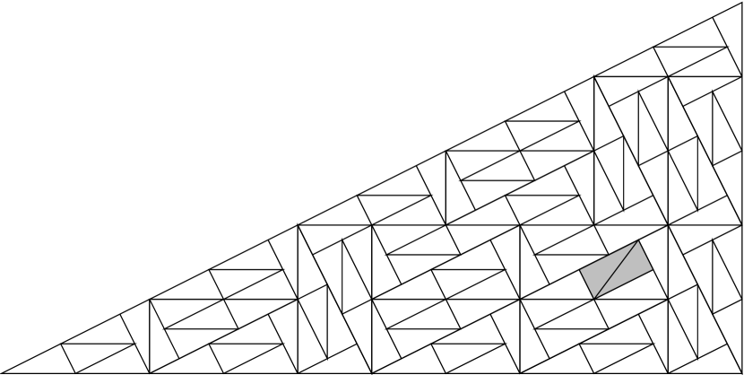
Figure 3. A right-handed 2-supertile expressed as a union of 125 1-supertiles. Only two of the 1-supertiles (shaded) are right-handed.

For each $\displaystyle(H,\theta)$, there is a supertile generated measure coming from the sequence of $\displaystyle N=2n$-supertiles of type $\displaystyle(H,\theta)$. Two such measures, one with $\displaystyle(H,\theta)$ and one with $\displaystyle(H^{\prime},\theta^{\prime})$, agree only if $\displaystyle H^{\prime}=H$ and if $\displaystyle\theta-\theta^{\prime}$ is a multiple of $\displaystyle\pi/2$. It is not hard to see that these measures are extreme points of $\displaystyle\Delta_{\infty}$, insofar as they maximize the frequency of $\displaystyle(H,\theta)$ tiles, and hence are ergodic.

For these ergodic measures, $\displaystyle\rho_{n}$ is atomic. If $\displaystyle n$ is even, then there is a large frequency of $\displaystyle(H,\theta+m\pi/2)$ $\displaystyle n$-supertiles, a smaller frequency of $\displaystyle(H,\theta\pm 2\alpha+m\pi/2)$, or of supertiles of the opposite handedness, a still smaller frequency with angle $\displaystyle\theta\pm 4\alpha\pm m\pi/2$, etc. There are countably many possibilities, but they occur with rapidly decreasing frequency.

However, the fusion rule is primitive, and hence the tiling space is minimal. Each $\displaystyle N$-supertile contains both right and left-handed $\displaystyle n$-supertiles, each in $\displaystyle 4(N-n-1)$ different directions. As $\displaystyle N\to\infty$, these directions become dense in $\displaystyle S^{1}$. For any $\displaystyle n$-supertile $\displaystyle P$ and any $\displaystyle\epsilon>0$, one can therefore find an $\displaystyle N$ such that every $\displaystyle N$-supertile contains an $\displaystyle n$-supertile with handedness and direction within $\displaystyle\epsilon$ of $\displaystyle P$.

This hybrid, like the pinwheel and (complete) anti-pinwheel spaces, has complexity that goes as $\displaystyle L^{3}/\epsilon^{3}$. As before, the number of possible directions of a supertile goes as $\displaystyle L/\epsilon$, while the number of locations for the origin goes as $\displaystyle L^{2}/\epsilon^{2}$.

A.3.1. A hybrid with totally disconnected transversal and strongly expansive dynamics

Since the fusion rule for the hybrid pinwheel-anti-pinwheel is rotationally invariant, there is an $\displaystyle S^{1}$ action on the transversal. In particular, the transversal is not disconnected. By modifying the construction to break this rotational invariance, we can get a tiling space that is minimal, has totally disconnected transversal, and is strongly expansive.

Let $\displaystyle C$ be a Cantor set obtained by disconnecting the circle at the countable set of points $\displaystyle n\alpha+m\pi/2\pmod{2\pi}$, where $\displaystyle n\in{\mathbb{Z}}$ and $\displaystyle\alpha=\arctan(1/2)$. That is, we remove each point $\displaystyle x$ of the form $\displaystyle n\alpha+m\pi/2$ from the circle and replace it with 2 points, $\displaystyle x^{+}$ considered as the limit from above and $\displaystyle x^{-}$ considered as a limit from below. For definiteness, pick a metric on $\displaystyle C$. There is an obvious continuous map from $\displaystyle C$ to $\displaystyle S^{1}$, and we call elements of $\displaystyle C$ “angles” and denote them $\displaystyle\theta$, with the understanding that some angles require a superscript. Note that addition of $\displaystyle\alpha$ is well-defined on $\displaystyle C$, sending $\displaystyle\theta^{\pm}$ to $\displaystyle(\theta+\alpha)^{\pm}$. Likewise, subtraction of $\displaystyle\alpha$ and addition of multiples of $\displaystyle\pi/2$ are well-defined.

Let $\displaystyle{\mathcal{P}}_{n}={\mathbb{Z}}_{2}\times C$, with the $\displaystyle n$-supertiles having the same supports as with the hybrid pinwheel. To the two points in $\displaystyle C$ with angle $\displaystyle\theta=k\alpha+m\pi/2$ we associate two different (super)tiles. These (super)tiles will have the same support but have different labels and may have different decompositions into lower-level supertiles.

For each $\displaystyle n>1$, consider a partition of $\displaystyle C$ into $\displaystyle 5^{2n-3}$ clopen sets, such that the diameter of these sets (in the metric on $\displaystyle C$) goes to zero uniformly as $\displaystyle n\to\infty$. To each of these clopen sets, associate a triangle in the anti-pinwheel decomposition of the $\displaystyle n$-supertile into $\displaystyle 5^{2n-2}$ smaller triangles.

To decompose an $\displaystyle n$-supertile of type $\displaystyle(H,\theta)$ into $\displaystyle(n-1)$-supertiles, first divide it into $\displaystyle 5^{2n-2}$ smaller triangles by applying the anti-pinwheel decomposition $\displaystyle 2n-2$ times. Then pick the triangle associated to $\displaystyle\theta$, and decompose it into 5 triangles using the pinwheel rule. Decompose the other $\displaystyle 5^{2n-2}-1$ triangles using the anti-pinwheel rule.

As a result of the $\displaystyle\theta$-dependence, this fusion rule breaks rotational symmetry and the rotation group does not act on $\displaystyle\Omega$. For any distinct $\displaystyle\theta_{1,2}\in C$, there exists an $\displaystyle n$ such that $\displaystyle\theta_{1}$ and $\displaystyle\theta_{2}$ are not in the same division of $\displaystyle C$ into $\displaystyle 5^{2n-3}$ clopen sets. This implies that an $\displaystyle n$-supertile of type $\displaystyle(H,\theta_{2})$ is combinatorially different from an $\displaystyle n$-supertile of type $\displaystyle(H,\theta_{1})$.

This makes the dynamics strongly expansive and makes the transversal totally disconnected. Two points $\displaystyle{\bf T}_{1}$ and $\displaystyle{\bf T}_{2}$ in the same transversal must have supertiles at some level that are different. This means that the combinatorics of the two tilings are different, so it is possible to find a clopen subset of the transversal, defined using combinatorial data, that contains $\displaystyle{\bf T}_{1}$ but not $\displaystyle{\bf T}_{2}$. Furthermore, there is a translation $\displaystyle x$ such that $\displaystyle{\bf T}_{1}$ and $\displaystyle{\bf T}_{2}$ differ by more than $\displaystyle\epsilon$, which establishes expansivity. To see that the tiling space is strongly expansive, note that the combinatorics of $\displaystyle{\bf T}_{1}$ and $\displaystyle{\bf T}_{2}$ are the same out to some distance and then are suddenly different; a time change could not account for the difference while preserving the match out to that point.

This example is minimal but not uniquely ergodic, for the exact same reasons that the hybrid pinwheel is minimal but not uniquely ergodic. The ergodic measures are obtained from sequences of $\displaystyle 2n$-supertiles with fixed $\displaystyle(H,\theta)$, and the complexity goes as $\displaystyle L^{3}/\epsilon^{3}$. The existence of uncountably many ergodic measures is evidence that this tiling space is not homeomorphic to an FLC tiling space.

A.4. A direct product variation with shears

We return to the tiling of Example 2 as an example of shear ILC. Each label set $\displaystyle{\mathcal{L}}_{n}$ consists of just four points, and the transition matrices $\displaystyle M_{n,n+1}$ all equal $\displaystyle\left[\begin{matrix}1&1&1&1\\ 3&0&3&0\\ 3&3&0&0\\ 9&0&0&0\end{matrix}\right]$. This means that the transition-consistency requirements on the measures $\displaystyle\rho_{n}$ are exactly the same as for an FLC substitution with the same matrix. Each $\displaystyle\rho_{n}$ must be proportional to the Perron-Frobenius eigenvector, $\displaystyle\left(\begin{smallmatrix}\lambda\cr 3\cr 3\cr-3\bar{\lambda}\end{smallmatrix}\right)$, where $\displaystyle\lambda=(1+\sqrt{13})/2$ and $\displaystyle\bar{\lambda}=(1-\sqrt{13})/2$. The measures of all literally admitted patches can then be recovered from equation (8), while the patches that appear in the limit have total frequency zero.

The measures $\displaystyle\rho_{n}$ are independent of the side length $\displaystyle\alpha$ (except for overall normalization constants). Perron-Frobenius theory tells us that each $\displaystyle\Delta_{n}$ consists of a single element, so by Theorem 4.5 this DPV must be uniquely ergodic.

However, the set of possible patches, and the count $\displaystyle\#(I\hbox{ in }P)$ on the right hand side of equation (8) very much do depend on $\displaystyle\alpha$. When $\displaystyle\alpha$ is rational, the tiling has FLC since if $\displaystyle\alpha=p/q$ then the offsets between neighboring tiles must be multiples of $\displaystyle 1/q$. In fact, all such multiples occur. Moreover, the offsets between neighboring $\displaystyle n$-supertiles is also all multiples of $\displaystyle 1/q$, up to the size of the supertiles in question. Despite being FLC, the complexity goes as $\displaystyle qL^{3}/\epsilon^{2}$, since the number of ways that two supertiles of size $\displaystyle L$ can meet is $\displaystyle qL$. As long as $\displaystyle L>\epsilon^{-1}>q$, $\displaystyle C(\epsilon,L)$ goes as $\displaystyle qL^{3}/\epsilon^{2}$.

When $\displaystyle\alpha$ is irrational, then the tiling has ILC [4], and the offsets between neighboring supertiles is arbitrary. A countable and dense set of offsets is literally admitted, a continuum of offsets appears in the limit, and the transversal has topological dimension 1. To distinguish patches to within $\displaystyle\epsilon$, we must specify the offset to within $\displaystyle\epsilon$, and there are $\displaystyle L/\epsilon$ ways to do so. $\displaystyle C(\epsilon,L)$ then goes as $\displaystyle L^{3}/\epsilon^{3}$. (This argument also applies to rational $\displaystyle\alpha$ when $\displaystyle\epsilon>1/q$. The distinction between rational and irrational $\displaystyle\alpha$ disappears when looking at structures of size greater than $\displaystyle 1/q$.)

A.5. A tiling of $\displaystyle{\mathbb{R}}$ with variable size tiles

We next consider a 1-dimensional tiling whose tiles appear in a continuum of sizes. The possible lengths of $\displaystyle n$-supertiles are $\displaystyle[{(3/2)^{n}},{3(3/2)^{n}}]$, and the fusion rule making an $\displaystyle n$-supertile depends on its length $\displaystyle x$. If $\displaystyle x$ is above a certain threshold (namely $\displaystyle 2(3/2)^{n}$), then it is composed of two $\displaystyle(n-1)$ supertiles, one of length $\displaystyle x/3$ and the other of length $\displaystyle 2x/3$. If $\displaystyle x$ is below the threshold the $\displaystyle n$-supertile is composed of one $\displaystyle(n-1)$ supertile, whose length is $\displaystyle x$, which we have ensured is an allowable $\displaystyle(n-1)$-supertile length.

We would like to allow the label sets of $\displaystyle n$-supertiles to be their possible lengths, but doing so would make the fusion rule discontinuous. To force continuity, we disconnect the line at each length $\displaystyle x$ of discontinuity, making two new points we call $\displaystyle x^{+}$ and $\displaystyle x^{-}$. The discontinuities happen for $\displaystyle x=3^{k}(3/2)^{m}$, where $\displaystyle k$ and $\displaystyle m$ are nonnegative integers; we call such values of $\displaystyle x$ special. If $\displaystyle x$ is special, then for small $\displaystyle\epsilon>0$ we say that $\displaystyle x-\epsilon$ is close to $\displaystyle x^{-}$ but not $\displaystyle x^{+}$, while $\displaystyle x+\epsilon$ is close to $\displaystyle x^{+}$ but not $\displaystyle x^{-}$. Our label sets are intervals $\displaystyle{\mathcal{L}}_{n}=[{(3/2)^{n}}^{+},{3(3/2)^{n}}^{-}]$ in the disconnected line, each of which breaks up into $\displaystyle O(n)$ ordinary closed intervals. (E.g., $\displaystyle[1^{+},3^{-}]=[1^{+},(3/2)^{-}]\cup[(3/2)^{+},(9/4)^{-}]\cup[(9/4)^{+},3^{-}]$.) These labels describe the lengths of the $\displaystyle n$-supertiles. 1-supertiles of label $\displaystyle 3^{+}$ and $\displaystyle 3^{-}$ each have length 3, but have different decompositions into ordinary tiles.

To extend the fusion rule described above to our newly labeled supertile sets, note that if $\displaystyle x$ is special, then either $\displaystyle x/3$ or $\displaystyle 2x/3$ is special (or both). In this case we use the $\displaystyle(n-1)$-supertiles with the same superscript as $\displaystyle x$ itself. Since $\displaystyle 2(3/2)^{n}=3(3/2)^{n-1}$ is special, we have eliminated the discontinuity in the rule.

The fusion rule is van Hove, recognizable, and primitive. Thus the tiling dynamical system is minimal and we may use Theorem 4.2 to determine the invariant measures. In the next few sections we will show that the system is uniquely ergodic and compute the invariant measure.

A.5.1. Transition-consistency

Lemma A.2.

Every transition-consistent and volume-normalized family of measures $\displaystyle\{\rho_{n}\}$ is non-atomic.

Proof.

Consider an $\displaystyle n$-supertile of size $\displaystyle x$. We will show that, for $\displaystyle N$ large, dividing an $\displaystyle N$-supertile of size $\displaystyle y$ into $\displaystyle n$-supertiles results in relatively few $\displaystyle n$-supertiles of label exactly $\displaystyle x$. Specifically, we will argue that the fraction of the $\displaystyle n$-supertile descendants that are of size $\displaystyle x$ is bounded above by a constant times $\displaystyle N^{-1/2}$, implying that no transition-consistent measure can give weight greater than $\displaystyle cN^{-1/2}$ to $\displaystyle n$-supertiles of label $\displaystyle x$. Since $\displaystyle N$ can be chosen arbitrarily large, the measure of the $\displaystyle n$-supertiles of label $\displaystyle x$ is zero.

If some of the descendants of $\displaystyle y$ have length $\displaystyle x$, then $\displaystyle y=x3^{k}(3/2)^{m}$ for some non-negative integers $\displaystyle k$ and $\displaystyle m$. Since $\displaystyle y/x$ is also approximately $\displaystyle(3/2)^{N-n}$, $\displaystyle N$ is bounded above and below by a constant times $\displaystyle k+m$. When dividing $\displaystyle y$, 2/3 of the length winds up in a chunk of size $\displaystyle 2y/3$ and 1/3 winds up in a chunk of size $\displaystyle y/3$. Dividing $\displaystyle k+m$ times, we get size $\displaystyle x$ only if we go to the larger daughter $\displaystyle m$ times and the smaller daughter $\displaystyle k$ times. There are at most $\displaystyle{k+m\choose m}$ ways to do this, so the fraction of the length of $\displaystyle y$ consisting of $\displaystyle n$-supertiles of type $\displaystyle x$ is at most $\displaystyle\left(\frac{1}{3}\right)^{k}\left(\frac{2}{3}\right)^{m}{k+m\choose m}$. This is the probability of getting $\displaystyle k$ heads and $\displaystyle m$ tails when flipping a biased coin $\displaystyle k+m$ times. Since the variance in the number of heads is proportional to the number of flips, and since the distribution is approximately normal (by the central limit theorem), the probability of getting exactly $\displaystyle k$ heads is bounded by a constant times $\displaystyle(k+m)^{-1/2}$, and hence by a constant times $\displaystyle N^{-1/2}$. ∎

Since $\displaystyle\rho_{n}$ is non-atomic, we can treat $\displaystyle\rho_{n}$ as a continuous measure on the (ordinary) interval $\displaystyle[(3/2)^{n},3(3/2)^{n}]$. We write

$$d\rho_{n}=f_{n}(x)dx,$$

to represent the frequency of $\displaystyle n$-supertiles whose lengths are between $\displaystyle x$ and $\displaystyle x+dx$. In principle, $\displaystyle\rho_{n}$ could have a singular component, in which case $\displaystyle f_{n}$ should be understood as a distribution rather than as an ordinary function.

Transition-consistency for the $\displaystyle\rho_{n}$s requires the $\displaystyle f_{n}$s to be related, which is key to computing the ergodic measure. By definition, for any measurable $\displaystyle I\subset{\mathcal{P}}_{n}$ we need

$$\int_{I}f_{n}(x)dx=\int_{y\in{\mathcal{P}}_{n+1}}M_{n,n+1}(I,y)f_{n+1}(y)dy.$$

To compute $\displaystyle M_{n,n+1}$ we identify three subsets of $\displaystyle{\mathcal{P}}_{n}$. If $\displaystyle x\in[{(3/2)^{n}}^{+},{(3/2)^{n+1}}^{-}]$, then the $\displaystyle n$-supertile of label $\displaystyle x$ must be the small daughter of an $\displaystyle(n+1)$-supertile of label $\displaystyle 3x$. An $\displaystyle n$-supertile with $\displaystyle x\in[{(3/2)^{n+1}}^{+},{2(3/2)^{n}}^{-}]$ must be the only child of an $\displaystyle(n+1)$ supertile of label $\displaystyle x$, and an $\displaystyle n$-supertile of length $\displaystyle x\in[{2(3/2)^{n}}^{+},{3(3/2)^{n}}^{-}]$ can either be the only child of an $\displaystyle(n+1)$-supertile of label $\displaystyle x$ or the large daughter of an $\displaystyle(n+1)$-supertile of label $\displaystyle 3x/2$. Thus, if $\displaystyle I\subset[{(3/2)^{n}}^{+},{(3/2)^{n+1}}^{-}]$ we see that $\displaystyle M_{n,n+1}(I,y)=\chi_{3I}(y)$ and we have

$$\int_{I}f_{n}(x)dx=\int_{3I}f_{n+1}(y)dy=\int_{I}3f_{n+1}(3x)dx,$$

implying that on this interval we have $\displaystyle f_{n}(x)=3f_{n+1}(3x)$. The computation for the other two intervals is similar and we obtain

$$f_{n}(x)=\begin{cases}3f_{n+1}(3x)&(3/2)^{n}\leq x\leq{(3/2)^{n+1}}\cr f_{n+1}(x)&{(3/2)^{n+1}}<x\leq{2(3/2)^{n}}\cr f_{n+1}(x)+(3/2)f_{n+1}(3x/2)&{2(3/2)^{n}<x\leq 3(3/2)^{n}.}\end{cases}$$

Because the transition-consistency relationship does not depend on $\displaystyle n$, we can renormalize all of the $\displaystyle f_{n}$’s and induce a map from $\displaystyle L^{2}([1,3])$ to itself. Define

$$\tilde{f}_{n}(x)=(3/2)^{2n}f_{n}((3/2)^{n}x).$$

The quantity $\displaystyle\tilde{f}_{n}(x)dx$ represents $\displaystyle(3/2)^{n}$ times the frequency of $\displaystyle n$-supertiles of length between $\displaystyle(3/2)^{n}x$ and $\displaystyle(3/2)^{n}(x+dx)$, and $\displaystyle x$ ranges from 1 to 3. Equivalently, if we were to rescale all lengths by $\displaystyle(3/2)^{n}$, it would represent the frequency (number per rescaled length) of $\displaystyle n$-supertiles of length between $\displaystyle x$ and $\displaystyle x+dx$.

The transition consistency equations become

$$\tilde{f}_{n}(x)=\begin{cases}(4/3)\tilde{f}_{n+1}(2x)&1\leq x\leq 3/2\cr(4/9)\tilde{f}_{n+1}(2x/3)&3/2<x\leq 2\cr(4/9)\tilde{f}_{n+1}(2x/3)+(2/3)\tilde{f}_{n+1}(x)&2<x\leq 3,\end{cases}$$

or equivalently $\displaystyle\tilde{f}_{n}(x)={\mathcal{T}}\tilde{f}_{n+1}(x)$, where

$${\mathcal{T}}\tilde{f}(x)=\begin{cases}(4/3)\tilde{f}(2x)&1\leq x\leq 3/2\cr(4/9)\tilde{f}(2x/3)&3/2<x\leq 2\cr(4/9)\tilde{f}(2x/3)+(2/3)\tilde{f}(x)&2<x\leq 3.\end{cases}$$

In the next section we see that $\displaystyle{\mathcal{T}}$ is a diagonalizable operator on $\displaystyle L^{2}([1,3])$ and compute its spectrum in order to show that there is a unique invariant measure.

A.5.2. The invariant measure

Theorem A.3.

The tiling space is uniquely ergodic, and the unique measure has

(11) $$\tilde{f}_{n}(x)=\begin{cases}\frac{c}{x^{2}}&x\leq 2\cr\cr\frac{3c}{x^{2}}&x>2,\end{cases}$$

for every $\displaystyle n$, where $\displaystyle c=(3\ln(3)-2\ln(2))^{-1}$.

Proof.

The proof follows the same general lines as the proof of Theorem 8 of [12]. To prove unique ergodicity, we show that the spectrum of $\displaystyle{\mathcal{T}}$ is entirely in the unit disk, that 1 is the only eigenvalue on the unit circle, and that there is a unique solution to $\displaystyle{\mathcal{T}}\tilde{f}=\tilde{f}$, up to normalization, namely the function listed above.

Suppose that $\displaystyle\tilde{f}$ is an eigenfunction of $\displaystyle{\mathcal{T}}$ with eigenvalue $\displaystyle\lambda$. The equations $\displaystyle{\mathcal{T}}\tilde{f}=\lambda\tilde{f}$ reduce to:

$$\displaystyle\tilde{f}(2x)/\tilde{f}(x)=3\lambda/4 \displaystyle\qquad 1\leq x\leq 3/2$$

$$\displaystyle\tilde{f}(2x/3)/\tilde{f}(x)=9\lambda/4 \displaystyle\qquad 3/2<x\leq 2$$

$$\displaystyle\tilde{f}(2x/3)/\tilde{f}(x)=3(3\lambda-2)/4 \displaystyle\qquad 2<x\leq 3$$

Note that $\displaystyle\tilde{f}(x)$ determines $\displaystyle\tilde{f}(2x)$ or $\displaystyle\tilde{f}(2x/3)$, which determines $\displaystyle\tilde{f}(4x/3)$ or $\displaystyle\tilde{f}(4x/9)$, which determines the next power of 2 times $\displaystyle x$, divided by an appropriate power of 3. At every stage, we add $\displaystyle\ln(2)$ to $\displaystyle\ln(x)\pmod{\ln(3)}$. Since $\displaystyle\tilde{f}(x)$ determines a dense set of function values, there is at most one function (up to scale) with eigenvalue $\displaystyle\lambda$. Irrational rotations yield a uniform measure on the circle, so we find ourselves in the range [1,3/2] a fraction $\displaystyle\ln(3/2)/\ln(3)$ of the time, in the range [3/2, 2] a fraction $\displaystyle\ln(4/3)/\ln(3)$ of the time and in the range [2,3] a fraction $\displaystyle\ln(3/2)/\ln(3)$ of the time, regardless of the initial value of $\displaystyle x$. This means that we multiply by $\displaystyle 3\lambda/4$ an average of $\displaystyle\ln(3/2)$ times for every $\displaystyle\ln(4/3)$ times that we multiply by $\displaystyle 9\lambda/4$ and for every $\displaystyle\ln(3/2)$ times that we multiply by $\displaystyle 3(3\lambda-2)/4$. Since the values of $\displaystyle\tilde{f}$ do not grow or shrink in the long run, we must have

(12) $$\left|\frac{3\lambda}{4}\right|^{\ln(3/2)}\left|\frac{9\lambda}{4}\right|^{\ln(4/3)}\left|\frac{3(3\lambda-2)}{4}\right|^{\ln(3/2)}=1,$$

or equivalently

(13) $$\ln(2)\ln|\lambda|+\ln(3/2)\ln|3\lambda-2|=0.$$

If $\displaystyle|\lambda|>1$, then both terms on the left hand side of (13) are positive. If $\displaystyle|\lambda|=1$ and $\displaystyle\lambda\neq 1$, the first term is zero and the second term is positive. Thus, the only possible eigenvalues are +1 and points that are strictly inside the unit circle.

It is straightforward to check that the function of equation (11) is in fact an eigenfunction of $\displaystyle{\mathcal{T}}$ with eigenvalue 1. The constant $\displaystyle c$ comes from the volume normalization condition $\displaystyle\int_{1}^{3}x\tilde{f}_{n}(x)dx=1$. ∎

Knowing the $\displaystyle\lambda=1$ eigenfunction is enough to determine the invariant measure. However, it is also useful to identify the other eigenvalues and eigenfunctions, as these describe how averages over finite regions can differ from the the ergodic limit. If $\displaystyle\gamma$ is a complex number such that

(14) $$3^{\gamma}=2^{\gamma}+1,$$

then the function:

$$\tilde{f}(x)=\begin{cases}x^{-(\gamma+1)}&1\leq x<2\cr 3^{\gamma}x^{-(\gamma+1)}&2<x\leq 3\end{cases}$$

is an eigenfunction of $\displaystyle{\mathcal{T}}$ with eigenvalue $\displaystyle\lambda=(3/2)^{\gamma-1}$. There are countably many solutions to (14), each corresponding to a solution to (12). (Condition (12) is necessary but not sufficient for $\displaystyle\lambda$ to be an eigenvalue.) 1 is an accumulation point for the spectrum of $\displaystyle{\mathcal{T}}$, so convergence under $\displaystyle{\mathcal{T}}$ to the unique invariant measure is not exponential.

A.5.3. Complexity and transversal

The complexity $\displaystyle C(\epsilon,L)$ goes as $\displaystyle L^{2}/\epsilon^{2}$. To specify a patch of size $\displaystyle L$ up to $\displaystyle\epsilon$ error, one must identify a supertile of size bigger than $\displaystyle L$, specify the length of the supertile to within $\displaystyle\epsilon$, and pick a location within that supertile to within $\displaystyle\epsilon$, leaving $\displaystyle L^{2}/\epsilon^{2}$ possibilities.

Despite having a continuum of tile lengths, this tiling space has totally disconnected transversal. The clopen sets describe the combinatorics of how tiles fit into supertiles of various orders out to a certain distance from the origin. To see this, imagine that tilings $\displaystyle T$ and $\displaystyle T^{\prime}$ are in the transversal and are close. This occurs when $\displaystyle T$ is, to a large distance, a small dilation of $\displaystyle T^{\prime}$ (or vice-versa). However, eventually $\displaystyle T^{\prime}$ will have a tile whose length is slightly less than $\displaystyle 3$, while the corresponding region of $\displaystyle T$, having length slightly greater than 3, consists of two tiles. Using this difference in combinatorics, we can construct a clopen set that contains $\displaystyle T$ but not $\displaystyle T^{\prime}$.

References

- [1] R. Benedetti and J.-M. Gambaudo, On the dynamics of G-solenoids: applications to Delone sets, Ergod. Th. Dyn. Sys. 23 (2003), 673–691.
- [2] L. Danzer, Inflation species of planar tilings which are not of locally finite complexity, Proc. Steklov Inst. Math. 230 (2002), 118–126.
- [3] T. Downarowicz, Survey of odometers and Toeplitz flows, Contemporary Mathematics 385 (2005) 7–37.
- [4] N. P. Frank and E. A. Robinson, Jr., Generalized -expansions, substitution tilings, and local finiteness, Trans. Amer. Math. Soc. 360 no. 3 (2008), 1163–1177.
- [5] N. P. Frank and L. Sadun, Topology of some tiling spaces without finite local complexity, Discrete Contin. Dyn. Syst. 23, no. 3 (2009), 847–865.
- [6] N.P. Frank and L. Sadun, Fusion: a general framework for hierarchical tilings of , Preprint 2011, arXiv:1101.4930, to appear in Geometriae Dedicata.
- [7] R.H. Herman, I. Putnam, and C. Skau, Ordered Bratteli diagrams, dimension groups, and topological dynamics, Int. J. Math. 3 (1992), 827-864.
- [8] R. Kenyon, Rigidity of planar tilings, Invent. math. 107 (1992), 637-651.
- [9] N. Ormes, C. Radin and L. Sadun, A homeomorphism invariant for substitution tiling spaces, Geometriae Dedicata 90 (2002), 153–182.
- [10] C. Radin, The pinwheel tilings of the plane, Annals of Math. 139:3 (1994), 661–702.
- [11] C. Radin and L. Sadun, Isomorphism of hierarchical structures, Ergod. Th. Dyn. Sys. 21 (2001), 1239-1248.
- [12] L. Sadun, Some generalizations of the pinwheel tiling, Disc. Comp. Geom. 20 (1998), 79-110.
- [13] L. Sadun, Tiling spaces are inverse limits, J. Mathematical Physics 44 (2003), 5410–5414
- [14] L. Sadun and R.F. Williams, Tiling spaces are Cantor set fiber bundles, Ergodic Theory and Dynamical Systems 23 (2003), 307–316.