Tetrahedral colloidal clusters from random parking of bidisperse spheres

Abstract

Using experiments and simulations, we investigate the clusters that form when colloidal spheres stick irreversibly to – or “park” on – smaller spheres. We use either oppositely charged particles or particles labeled with complementary DNA sequences, and we vary the ratio $\alpha$ of large to small sphere radii. Once bound, the large spheres cannot rearrange, and thus the clusters do not form dense or symmetric packings. Nevertheless, this stochastic aggregation process yields a remarkably narrow distribution of clusters with nearly 90% tetrahedra at $\alpha=2.45$. The high yield of tetrahedra, which reaches 100% in simulations at $\alpha=2.41$, arises not simply because of packing constraints, but also because of the existence of a long-time lower bound that we call the “minimum parking” number. We derive this lower bound from solutions to the classic mathematical problem of spherical covering, and we show that there is a critical size ratio $\alpha_{c}=(1+\sqrt{2})\approx 2.41$, close to the observed point of maximum yield, where the lower bound equals the upper bound set by packing constraints. The emergence of a critical value in a random aggregation process offers a robust method to assemble uniform clusters for a variety of applications, including metamaterials.

Understanding the geometry of clusters formed from small particles is a fundamental problem in condensed matter physics, with implications for phenomena ranging from nucleation Kelton et al. (2003) to self-assembly Manoharan et al. (2003). Colloidal particles are a useful experimental system for studying cluster geometry and its relation to phase behavior Gasser et al. (2001) for several reasons: they are large enough to be directly observed using optical microscopy; their assembly can be understood in terms of geometry Arkus et al. (2009); Hoy and O’Hern (2010); and they can be driven to cluster by a variety of controllable interactions, including capillary forces Manoharan et al. (2003), depletion Meng et al. (2010), fluctuation-induced forces Yunker et al. (2011), or DNA-mediated attraction Soto et al. (2002). Colloidal clusters are also useful materials in their own right. They can be used, for example, as building blocks for isotropic optical metamaterials known as metafluids Urzhumov et al. (2007); Alù and Engheta (2009); Fan et al. (2010). Tetrahedral clusters are of particular interest for metafluids since the tetrahedron is the simplest cluster with isotropic dipolar symmetry Urzhumov et al. (2007). An unsolved challenge for this application is to determine the interactions and conditions that enable assembly of bulk quantities of highly symmetric, uniform clusters such as tetrahedra.

With this motivation in mind, we study experimentally the geometry and size distribution of binary clusters formed when small colloidal spheres are mixed with an excess of large spheres that stick irreversibly and randomly to their surfaces (Figure 1a). An obvious way to control the cluster geometry in such binary systems is to vary the size ratio. One might expect that at certain ratios the particles could arrange into dense clusters or “spherical packings” – arrangements of spheres around a central sphere that maximize surface density Melnyk et al. (1977); Conway and Sloane (1993); Phillips et al. (2012). Such packings have long been used in modeling the microstructure of dense, disordered atomic systems Egami (1997); Miracle (2004). But unlike atoms, colloidal particles can stick irreversibly, such that two particles bound to a third show no motion relative to one another. This type of binding occurs frequently in strongly interacting, monodisperse colloidal suspensions, which consequently form fractal aggregates instead of dense glasses Weitz and Oliveria (1984); Lin et al. (1989). Similarly, in the binary systems we study, the irreversible and stochastic process of sticking precludes the formation of dense or symmetric packings. The large spheres park, rather than pack, on the surfaces of the small spheres.

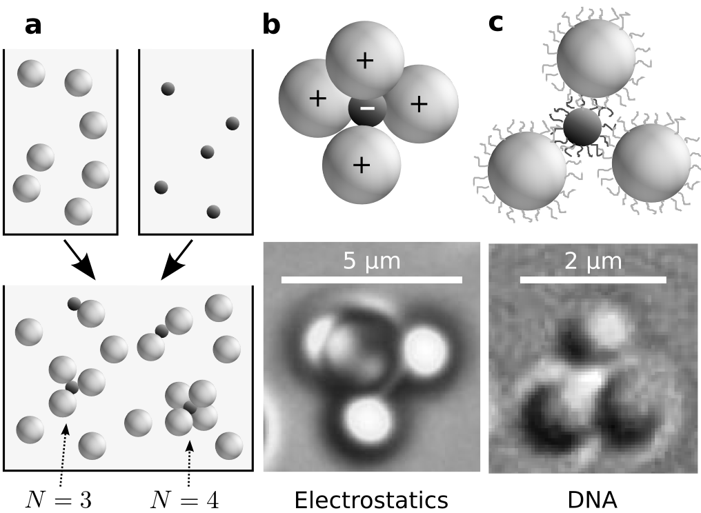
Figure 1: (a) Two colloidal sphere species are mixed together to form clusters. (b) Oppositely charged polystyrene spheres cluster due to electrostatic attraction. Optical micrograph shows a tetramer ($N=4$). (c) Polystyrene spheres labeled with complementary DNA strands (not to scale) cluster due to DNA hybridization. Optical micrograph shows a trimer ($N=3$); the small, central sphere is fluorescent.

Surprisingly, this random and non-equilibrium process can produce clusters of uniform size. Our experiments show that at a size ratio $\alpha=R_{\mathrm{big}}/R_{\mathrm{small}}=2.45$, where $R_{\mathrm{big}}$ and $R_{\mathrm{small}}$ are the sphere radii, nearly all of the clusters contain four large spheres stuck to a smaller sphere (Table 1). In these experiments we use a 100:1 stoichiometric ratio of the two sphere species, statistically ensuring that each cluster contains only one small sphere surrounded by two or more larger spheres. After waiting several days for the average cluster size to saturate, we measure the distribution of $N$, the number of large spheres bound to each small sphere . We do not count single large spheres, nonspecifically aggregated clusters of large spheres, or clusters with multiple small spheres. While there are many isolated large spheres due to the high stoichiometric ratio, the latter two types of cluster are rare.

Size ratio $\alpha$	1.94	2.45	3.06	4.29
$N=6$	6.3	0.0	0.0	0.0
$N=5$	39.2	0.8	0.0	0.0
$N=4$	54.4	90.2	18.6	0.7
$N=3$	0.0	6.6	69.9	35.9
$N=2$	0.0	0.8	10.9	51.0
$N=1$	0.0	0.8	0.6	11.1
$N=0$	0.0	0.8	0.0	1.3

Table 1: Experimentally observed cluster size distributions for charged colloids. Percentages of total are listed. The distribution for $\alpha=2.45$ (red) is sharply peaked at $N=4$.

The $N=4$ tetramers that we observe are not dense packings or, in general, symmetric arrangements. As can be seen from the images in Figure 1, there is space between the large particles, and the resulting tetrahedra are irregular. Moreover, the ratio $\alpha=2.45$ is well below the value $\alpha=4.44$ found by Miracle et al. Miracle et al. (2003) for efficient tetrahedral packing in binary atomic clusters. In fact, at $\alpha=4.29$, closer to this bound, we see much smaller clusters and few tetrahedra. The sparsity of large spheres in the clusters is a result of the irreversible, non-equilibrium, random binding: once the big particles stick to the smaller ones, we do not see them detach or move relative to one another. We expected such a stochastic process to lead to a much broader distribution of clusters. At other values of $\alpha$ it does (Table 1), but at $\alpha=2.45$ we obtain 90% tetramers.

The high yield of tetramers occurs in two experimental systems with different types of interactions. In both systems the interactions are specific, strong, and short-ranged, and the particles do not rearrange once bound. In the first system the clustering is driven by electrostatic interactions. We mix large, positively-charged particles with small, negatively-charged particles, as shown in Figure 1b. To adjust $\alpha$, we use several different particle sizes . We add salt to reduce the Debye length to approximately $3\text{\,}\mathrm{nm}$, small enough to ensure that the interaction range does not significantly influence the effective particle size. In the second system the clustering is driven by hybridization of grafted DNA strands . As shown in Figure 1c, we mix small and large spheres labeled with complementary DNA oligonucleotides Dreyfus et al. (2009). We work well below the DNA melting temperature so that the attractive interaction is many times the thermal energy Dreyfus et al. (2010).

To better understand why the distribution is sharply-peaked at $N=4$ for $\alpha=2.45$, we use simulations and analytical techniques that account for the irreversibility of the aggregation process. Our simulations use a “random parking” algorithm Mansfield et al. (1996); Rosen et al. (1986); Wouterse et al. (2005); Talbot et al. (2000) to model the formation of clusters. The algorithm involves attaching large spheres to randomly selected positions on the surface of a small sphere, subject to a no-overlap constraint . We do not model the finite range of the interactions, which in both experimental systems is small compared to the particle size, or the diffusion of the particles prior to binding. In accord with experimental observations, the particles are not allowed to rearrange once bound. We repeat the process numerically to obtain distributions of cluster sizes as a function of a single parameter, $\alpha$.

The simulations find a 100% yield of tetramers at the size ratio $\alpha\approx 2.41$. As in the experiments, the large particles in these tetramers are not densely packed, and the clusters are therefore distorted tetrahedra. We also find that while the yield of any particular cluster can be maximized by varying $\alpha$ (Figure 2a), the yield approaches 100% only for dimers ($N=2$) and tetramers ($N=4$). Interestingly, the yield curve for tetramers has a cusp at its peak, showing that the size ratio $\alpha_{c}$ at the maximum is a mathematical critical point.

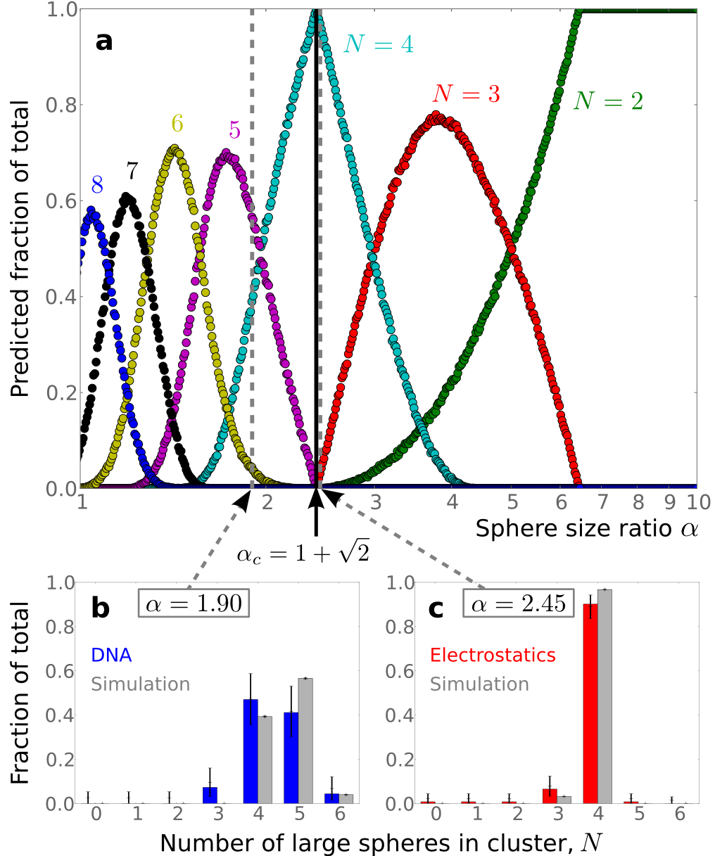
Figure 2: (a) Yield curves, as determined by simulations, for $N$-particle clusters, $2\leq N\leq 8$, where the critical size ratio $\alpha_{c}$ is marked with a black line. Below are histograms for (b) DNA-labeled particles (blue) at $\alpha=1.90$ and (c) charged particles (red) at $\alpha=2.45$, as observed in experiments and as predicted from simulations (gray). Error bars are 95% confidence intervals (Wilson score interval method).

The simulated distributions agree well with those found experimentally (Figure 2b,c) for both electrostatic and DNA-mediated interactions. For instance, at $\alpha=2.45$ with electrostatic interactions, we find a sharply-peaked distribution consisting almost entirely of tetramers. This value of $\alpha$ is close to but not precisely at the critical value, so a small yield of trimers is predicted and observed experimentally. In contrast, at $\alpha=1.90$ we find a mixture of mostly $N=4$ and $N=5$ clusters in both the DNA system and simulations. Some discrepancy arises between the simulated and experimental histograms because the yield curves in Figure 2a are steep; a slight error in the effective size ratio can shift the cluster distribution. Nevertheless, the random sphere parking model successfully reproduces both the large yield of tetrahedra near $\alpha_{c}$ and the details of the measured histograms at various other $\alpha$.

That we can reproduce the same phenomenon in two different experimental systems and in a one-parameter model suggests that the critical size ratio $\alpha_{c}$ has a universal, geometrical origin. Intuitively one might expect that it is related to packing constraints on the large spheres. Other theoretical studies of random sphere parking Rosen et al. (1986); Mansfield et al. (1996) have calculated the maximum number of large spheres $N_{\max}$ that can fit around a small sphere at a given $\alpha$. However, this bound cannot by itself explain why the yield of tetramers can reach 100% while that of other clusters, such as trimers or hexamers, cannot. At a given $\alpha$, it tells us only why no clusters larger than $N_{\max}(\alpha)$ can form, but it says nothing about the probability of forming smaller clusters with different arrangements.

Therefore we also examine a different bound, one not previously discussed in the context of random sphere parking: the “minimum parking” curve $N_{\min}(\alpha)$. $N_{\min}$ is the smallest number of hard spheres that can be positioned on a smaller sphere such that another sphere cannot fit. To understand this bound, consider a simple, one-dimensional analogy to car parking on a busy city street, where if a space opens up that is large enough to fit a car, it is filled. The minimum parking number occurs when all drivers have been equally inconsiderate, leaving spaces between their parked cars that are all slightly too small for another car to fit. This lower bound is meaningful only at long times, when all available parking spaces have been filled. The long-time limit holds also for our experiments and simulations, which we carry out until the average cluster size has saturated.

Whereas the upper bound $N_{\max}(\alpha)$ is straightforwardly related to solutions of the well-known spherical packing problem Conway and Sloane (1993); Sloane et al. (2011), the calculation of the lower bound $N_{\min}(\alpha)$ requires a different approach. In our clusters, the distance between the centers of any two big spheres must be at least $2R_{\mathrm{big}}$. Consider then a sphere of radius $(R_{\mathrm{small}}+R_{\mathrm{big}})$ that circumscribes the centers of the parked spheres. If this sphere is completely covered with $N$ circles of radius $2R_{\mathrm{big}}$, it will be impossible to add an $(N+1)^{\mathrm{th}}$ large sphere. We are led naturally to the spherical covering problem, a problem with a rich history in mathematics. Like spherical packings, spherical coverings are solutions to an extremum problem: they are arrangements of $N$ points on a sphere that minimize the largest distance between any location on the sphere surface and the closest point Conway and Sloane (1993). But unlike spherical packings, spherical coverings need not correspond to arrangements of non-overlapping spheres. We therefore solve for the minimum parking curve by examining the solutions to the spherical covering problem Sloane et al. (2011) at each $N$ and manually verifying that they correspond to non-overlapping configurations .

Our analytical results for the bounds reveal why $\alpha_{c}$ is a special point: it is the only non-trivial point where the calculated maximum and minimum parking curves come together (Figure 3). Analytically we find the location of the critical value to be $\alpha_{c}=(1+\sqrt{2})\approx 2.41$, very close to the values where the experimental distributions are peaked. At $\alpha$ slightly larger than this value, the minimum parking configuration corresponds to two spheres placed at opposite poles ($N_{\min}=2$), and the maximum $N$ is obtained by first parking three large spheres next to one another, so that there is room for one more sphere to park ($N_{\max}=4$). At $\alpha$ slightly smaller than $\alpha_{c}$, the big spheres can park along orthogonal axes about the small sphere to make an octahedron ($N_{\max}=6$). The minimum $N$ is obtained by placing four spheres as far from each other as possible, so as to make the addition of a fifth impossible ($N_{\min}=4$). Thus as we increase $\alpha$ through $\alpha_{c}$, $N_{\max}$ goes from $6$ to $4$ and $N_{\min}$ from $4$ to $2$, and the two curves become infinitesimally close.

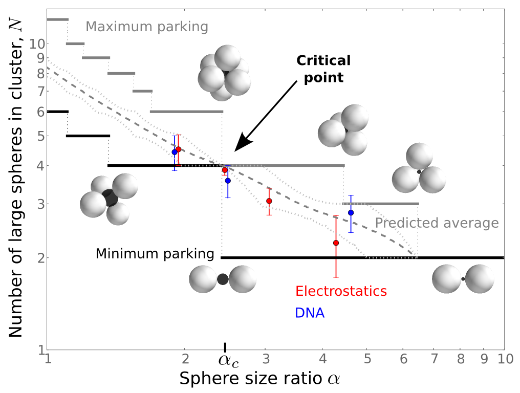
Figure 3: $N_{\max}$ (solid gray) and $N_{\min}$ (black) as functions of $\alpha$. Cluster images show sphere configurations at discontinuities of these curves. Average cluster sizes from simulations (dashed gray) and experiments (blue and red data points) are shown. We characterize the statistical dispersion in each distribution by the average absolute deviation from the median, indicated by dotted light gray lines for simulations and vertical bars for experiments.

The parking process is therefore geometrically constrained to yield clusters with exactly $N=4$ particles in the limit $\alpha\rightarrow\alpha_{c}$. A simple geometric argument sheds some light on this result. At $\alpha_{c}$ there is always room for four large spheres to park. Parking more spheres requires that at least three park precisely along a great circle of the smaller particle, but the probability of this happening randomly is zero. Thus irreversible binary aggregation, a stochastic process, has a deterministic feature at the critical size ratio: although the space between the large spheres can vary, all clusters must be tetramers. Our numerical approach confirms that the statistical dispersion in the cluster size distribution vanishes at $\alpha_{c}$, as shown in Figure 3.

The experimental and simulated distributions differ slightly due to two effects. First, the measured sizes tend to be smaller than the simulated ones because a few parking spaces remain unfilled even at long times. This effect is more pronounced for larger spheres, which diffuse more slowly and encounter the small spheres less frequently. The systems most affected are the electrostatic ones at $\alpha=3.06$ and $4.29$. Second, the experimental size ratios can vary by 5% due to polydispersity. Both of these factors increase the width in the experimental distributions and diminish the achievable yield of tetramers near $\alpha_{c}$. Nevertheless, the experimental data indicate that near $\alpha_{c}$ a tetramer yield of at least 90% is possible, and, although the model does not account for the finite range of the interactions or the diffusivity of the particles, it is useful for predicting cluster size distributions in two very different colloidal systems.

These results have both fundamental and practical consequences. On the fundamental side, the particle size ratio could affect the jamming threshold in bulk packings of bidisperse spheres. Previous simulations of these systems have shown that the distribution of coordination numbers also depends on the size ratio He et al. (1999) and may be modeled using random parking Wouterse et al. (2005). This contrasts with dense atomic systems like metallic glasses Egami (1997); Miracle (2004) in which the atoms have some freedom to rearrange locally. In these systems packing constraints may explain structure and coordination better than parking arguments.

On the practical side, this random aggregation process is a simple way to mass produce tetrahedral clusters in theoretically 100% yield. Although the tetrahedra we produce are irregular in that the distance between the large spheres can vary, it may well be possible to form large quantities of symmetric tetrahedra simply by shrinking the small spheres after the tetramers have formed Lyon et al. (2004). Furthermore, although the yield will approach 100% only for dimers and tetramers, the yield of any $N$-particle cluster can be maximized by choosing the appropriate size ratio. For instance, the yield of octahedral clusters, also promising candidates for building metamaterials Alù and Engheta (2009), may surpass 70% at $\alpha=1.42$.

The size ratio in binary colloidal systems thus emerges as a valuable control parameter for directed self-assembly. Moreover, because it does not require precise control over the interactions, random parking offers a robust and simple way to make colloidal clusters that are more monodisperse than those prepared through other methods Manoharan et al. (2003).

We thank W. Benjamin Rogers, Rodrigo Guerra and Michael P. Brenner for helpful discussions. This work was funded by the National Science Foundation NIRT program (grant no. ECCS-0709323) and the Harvard MRSEC (grant no. DMR-0820484). NBS acknowledges support from the Department of Energy Office of Science Graduate Fellowship Program, administered by ORISE-ORAU under contract no. DE-AC05-06OR23100.

I Electrostatic interaction experiments

Charged colloidal polystyrene spheres were purchased from Invitrogen as “IDC surfactant-free latex” in batches as listed in Table 2.

Mean diameter	Surface functionality	Fluorescent?	Surface charge
$0.49\text{\,}\mathrm{\SIUnitSymbolMicro m}$	carboxylate-modified latex (CML)	yes	$-262\text{\,}\mathrm{\SIUnitSymbolMicro}\mathrm{C}\mathrm{/}\mathrm{c}\mathrm{m}^{2}$
$0.95\text{\,}\mathrm{\SIUnitSymbolMicro m}$	amidine	no	$+23.7\text{\,}\mathrm{\SIUnitSymbolMicro}\mathrm{C}\mathrm{/}\mathrm{c}\mathrm{m}^{2}$
$1.2\text{\,}\mathrm{\SIUnitSymbolMicro m}$	amidine	no	$+18.2\text{\,}\mathrm{\SIUnitSymbolMicro}\mathrm{C}\mathrm{/}\mathrm{c}\mathrm{m}^{2}$
$1.5\text{\,}\mathrm{\SIUnitSymbolMicro m}$	aldehyde-amidine	no	$+18.2\text{\,}\mathrm{\SIUnitSymbolMicro}\mathrm{C}\mathrm{/}\mathrm{c}\mathrm{m}^{2}$
$2.1\text{\,}\mathrm{\SIUnitSymbolMicro m}$	amidine	no	$+30.2\text{\,}\mathrm{\SIUnitSymbolMicro}\mathrm{C}\mathrm{/}\mathrm{c}\mathrm{m}^{2}$

Table 2: Charged particles used in electrostatic system experiments. Values for surface charge from data sheets provided by manufacturers.

A $100\text{\,}\mathrm{\SIUnitSymbolMicro L}$ sample of each colloid was diluted to 1% weight by volume. This was then vortexed for a few seconds and bath-sonicated for 10 seconds. We cleaned the particles by centrifuging and redispersing them several times in deionized (DI) water, using the following wash procedure.

1. Colloids were centrifuged for 5 minutes at 6600g.

2. Supernatant was removed and $190\text{\,}\mathrm{\SIUnitSymbolMicro L}$ of DI water were added to each sample.

3. Samples were vortexed for 5 seconds each and then bath-sonicated for 10 seconds.

We performed six wash cycles. After the last centrifugation, the supernatant was replaced with $40\text{\,}\mathrm{\SIUnitSymbolMicro L}$ of DI water, rather than $190\text{\,}\mathrm{\SIUnitSymbolMicro L}$ as before. Then $50\text{\,}\mathrm{\SIUnitSymbolMicro L}$ of 20 mM NaCl were added to each sample to achieve an overall salt concentration of 10 mM. This screens the repulsion between like particles before mixing.

We prepared mixtures of the positively and negatively charged particles such that each mixture contained one batch of positively charged particles at 1% w/v. In each mixture, the number ratio of the large (positively charged) to small (negatively charged) spheres was $100:1$. The salt concentration in each mixture was 10 mM NaCl. Each mixture consisted of large and small particles with a different size ratio $\alpha$, as listed in Table 3.

$\alpha$	Large particles	Small particles
$1.94$	$0.95\text{\,}\mathrm{\SIUnitSymbolMicro m}$ amidine (+)	$0.49\text{\,}\mathrm{\SIUnitSymbolMicro m}$ CML (-)
$2.45$	$1.2\text{\,}\mathrm{\SIUnitSymbolMicro m}$ amidine (+)	$0.49\text{\,}\mathrm{\SIUnitSymbolMicro m}$ CML (-)
$3.06$	$1.5\text{\,}\mathrm{\SIUnitSymbolMicro m}$ aldehyde-amidine (+)	$0.49\text{\,}\mathrm{\SIUnitSymbolMicro m}$ CML (-)
$4.29$	$2.1\text{\,}\mathrm{\SIUnitSymbolMicro m}$ amidine (+)	$0.49\text{\,}\mathrm{\SIUnitSymbolMicro m}$ CML (-)

Table 3: Size ratios and components of binary mixtures of charged colloids.

Each mixture was stored in a micro-centrifuge tube and vortexed at 3,000 RPM, bath-sonicated for 20 seconds, and then mounted on a Glas-Col Rugged Rotator to tumble slowly at 4^∘C. Each mixture tumbled for at least three days before observation to reduce the effects of sedimentation on local particle concentrations throughout the mixture. To make it easier to identify and characterize one cluster at a time, we diluted samples of the mixtures to 0.1% w/v just prior to observing the distribution of cluster sizes.

I.1 Electrostatics control experiment

In the experiments outlined above, each mixture contained particles with surface charges of opposite sign. In a separate control experiment, we mixed particles of two different sizes but with surface charges of the same sign. Both components in our control mixture were carboxylate-modified latex (CML) colloids with a size ratio $\alpha=2.24$, as listed in Table 4.

Mean diameter	Surface functionality	Fluorescent?	Surface charge
$0.49\text{\,}\mathrm{\SIUnitSymbolMicro m}$	CML	yes	$-262\text{\,}\mathrm{\SIUnitSymbolMicro}\mathrm{C}\mathrm{/}\mathrm{c}\mathrm{m}^{2}$
$1.1\text{\,}\mathrm{\SIUnitSymbolMicro m}$	CML	no	$-31.5\text{\,}\mathrm{\SIUnitSymbolMicro}\mathrm{C}\mathrm{/}\mathrm{c}\mathrm{m}^{2}$

Table 4: Colloids used in electrostatic system control experiment.

These colloids were washed using the procedure outlined above and then mixed in a $100:1$ number ratio. After tumbling at 4^∘C for several days, the cluster size distribution was measured. As shown in Figure 4, fewer than 1% of the small particles bind to large particles when they have surface charges of the same sign. Nonspecific aggregation is therefore rare in the charged colloidal systems.

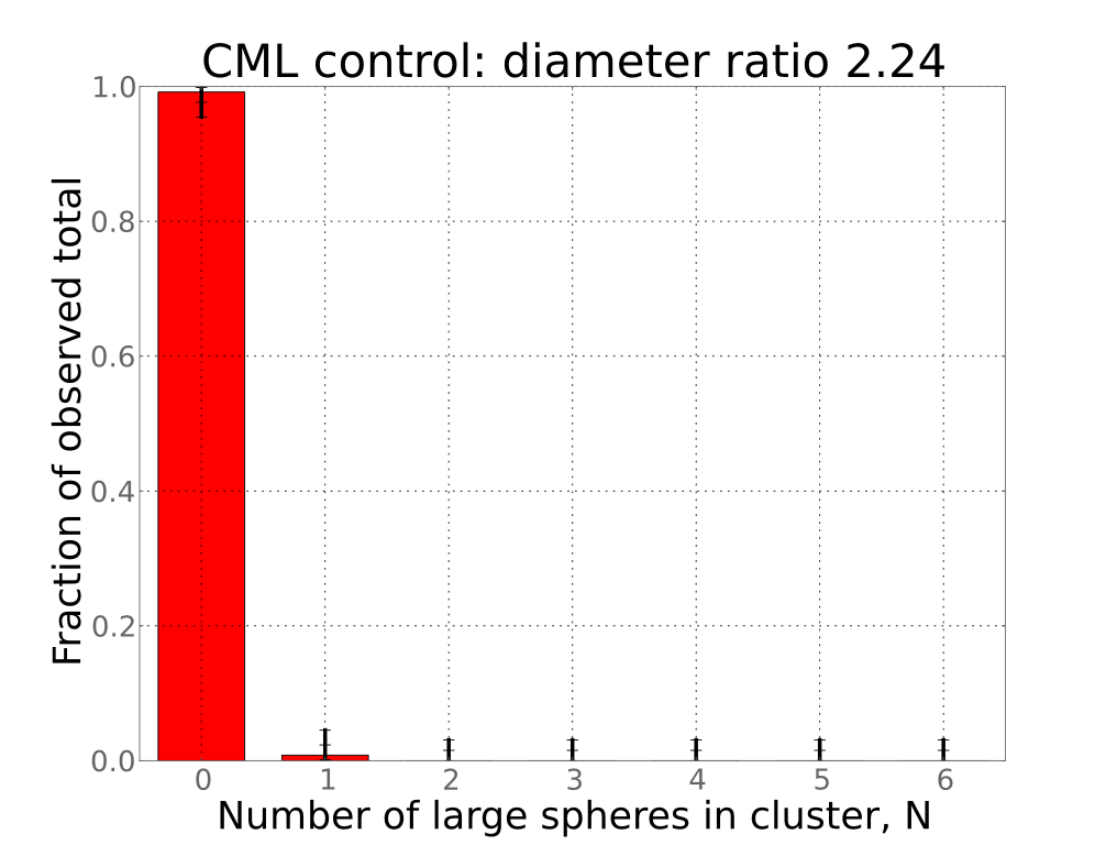
Figure 4: Cluster size distribution in a mixture of $1.1\text{\,}\mathrm{\SIUnitSymbolMicro m}$ non-fluorescent CML particles and $0.49\text{\,}\mathrm{\SIUnitSymbolMicro m}$ fluorescent CML particles in a $100:1$ number ratio, showing that particles with surface charge of the same sign rarely form clusters.

I.2 Experiments without salt

In another set of experiments, mixtures of charged colloidal particles were prepared as described above, but without salt. The number ratio of positively charged spheres to negatively charged spheres was again $100:1$, and several size ratios $\alpha$ were investigated, as listed in Table 5. As in the experiments with 10 mM NaCl, we tumbled the mixtures for several days before measuring the distribution of clusters.

$\alpha$	Large particles	Small particles
$1.09$	$1.2\text{\,}\mathrm{\SIUnitSymbolMicro m}$ amidine (+)	$1.1\text{\,}\mathrm{\SIUnitSymbolMicro m}$ CML (-)
$1.36$	$1.5\text{\,}\mathrm{\SIUnitSymbolMicro m}$ aldehyde-amidine (+)	$1.1\text{\,}\mathrm{\SIUnitSymbolMicro m}$ CML (-)
$1.94$	$0.95\text{\,}\mathrm{\SIUnitSymbolMicro m}$ amidine (+)	$0.49\text{\,}\mathrm{\SIUnitSymbolMicro m}$ CML (-)
$2.45$	$1.2\text{\,}\mathrm{\SIUnitSymbolMicro m}$ amidine (+)	$0.49\text{\,}\mathrm{\SIUnitSymbolMicro m}$ CML (-)
$3.06$	$1.5\text{\,}\mathrm{\SIUnitSymbolMicro m}$ aldehyde-amidine (+)	$0.49\text{\,}\mathrm{\SIUnitSymbolMicro m}$ CML (-)
$4.29$	$2.1\text{\,}\mathrm{\SIUnitSymbolMicro m}$ amidine (+)	$0.49\text{\,}\mathrm{\SIUnitSymbolMicro m}$ CML (-)

Table 5: Size ratios and components of binary mixtures without salt.

Figure 5 shows that the average cluster sizes in these mixtures were smaller than the average sizes predicted from simulation and those observed in mixtures containing 10 mM NaCl. For instance, at $\alpha=2.45$ with 10 mM NaCl the average cluster size is $N=3.9$, but when there is no salt in the system the average cluster size is $N=2.7$. For the four size ratios for which there is data both without salt and with 10 mM NaCl, we found that clusters are 20% to 35% smaller when no salt is added.

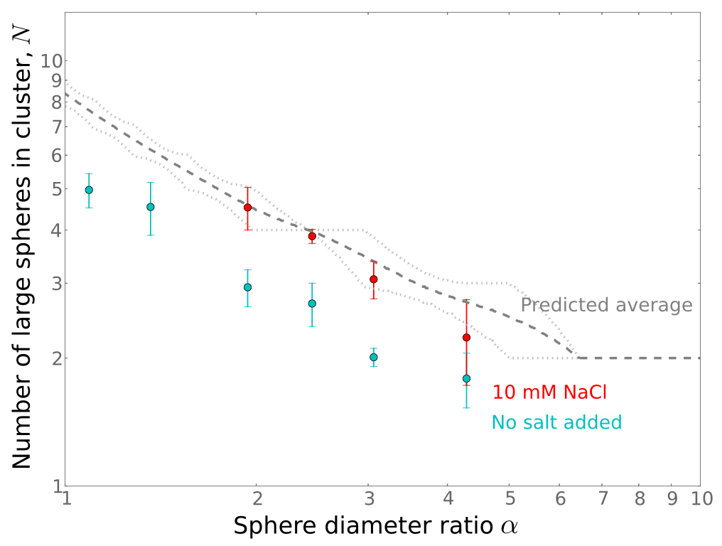
Figure 5: Average cluster sizes from simulations (dashed dark gray) and electrostatic experiments with (red data points) and without (cyan) salt. Widths of the cluster size distributions are indicated by dotted light gray lines for simulations and vertical error bars for experiments.

These experiments show that electrostatic repulsion affects the cluster assembly. This observation is consistent with other recent experiments Wang et al. (2010) showing that the cluster size distribution in binary mixtures depends on ionic strength when the salt concentration is less than 10 mM. In our mixtures with 10 mM NaCl, the Debye length is approximately $3\text{\,}\mathrm{nm}$, very small compared to the particle sizes, so the large spheres do not interact with each other except at small distances. The random parking model should be more appropriate for systems like these where the interaction range is much smaller than the particle size. This is because the random parking model assumes no interactions between the particles except for a hard-core repulsion and irreversible binding on contact between spheres of two different types.

II DNA-colloid experiments

In another set of experiments, we mixed small and large spheres labeled with complementary 65-base ssDNA oligonucleotides purchased from Integrated DNA Technologies:

• Sequence A: 5’-biotin-51xT-TGTTGTTAGGTTTA-3’

• Sequence B: 5’-biotin-51xT-TAAACCTAACAACA-3’

The oligonucleotides terminate with a biotin group, which allows us to graft them to streptavidin-coated polystyrene particles using a protocol from Dreyfus et al. Dreyfus et al. (2009). The streptavidin-coated polystyrene particles are purchased from Bangs Laboratories, Inc. with the following diameters:

• $0.21\text{\,}\mathrm{\SIUnitSymbolMicro m}$, fluorescent, to be coated with sequence B

• $0.39\text{\,}\mathrm{\SIUnitSymbolMicro m}$, fluorescent, to be coated with sequence B

• $0.51\text{\,}\mathrm{\SIUnitSymbolMicro m}$, fluorescent, to be coated with sequence B

• $0.97\text{\,}\mathrm{\SIUnitSymbolMicro m}$, non-fluorescent, to be coated with sequence A

DNA strands were dissolved in water in $20\text{\,}\mathrm{\SIUnitSymbolMicro}$M concentration. $20\text{\,}\mathrm{\SIUnitSymbolMicro L}$ of this DNA solution were mixed with $10\text{\,}\mathrm{\SIUnitSymbolMicro L}$ of 1% w/w streptavidin-coated polystyrene particles with $120\text{\,}\mathrm{\SIUnitSymbolMicro L}$ of phosphate buffer in a 1.7 mL propylene micro-centrifuge tube. Each 50 mL batch of buffer contained 0.0128 g KH₂PO₄, 0.0707 g K₂HPO₄, 0.1467 g NaCl, and 0.250 g F108 surfactant in 50 mL of deionized water. The buffer was filtered through a $0.2\text{\,}\mathrm{\SIUnitSymbolMicro m}$ membrane before use. A separate batch containing no salt was also prepared so that the salt concentration could be adjusted by combining the two. Mixtures were vortexed at 3,000 RPM for 5 seconds and bath-sonicated for 10 seconds. They were incubated at room temperature for 30 minutes to allow the ssDNA to graft to the surface of the particles. Then we washed the colloids using the following procedure:

1. Colloids were centrifuged for 3 minutes at 12,000g.

2. Supernatant was removed and $100\text{\,}\mathrm{\SIUnitSymbolMicro L}$ of 50 mM NaCl buffer were added to each sample.

3. Samples were vortexed for 5 seconds each at 3,000 RPM and then bath-sonicated for 10 seconds.

We washed each colloid three times to remove excess DNA from the system, and then incubated each at 55^∘C for 30 minutes. We then washed three more times, incubated at 55^∘C for another 30 minutes, and washed three times again. At this point the salt concentration in the buffer was adjusted to 20 mM. The A- and B-labeled particles were mixed in a $100:1$ (large : small) number ratio such that the larger particles were at a volume fraction of about 0.1%. Three separate mixtures were prepared, as listed in Table 6.

$\alpha$	Large particles	Small particles
$1.90$	$0.97\text{\,}\mathrm{\SIUnitSymbolMicro m}$, sequence A	$0.51\text{\,}\mathrm{\SIUnitSymbolMicro m}$, sequence B
$2.49$	$0.97\text{\,}\mathrm{\SIUnitSymbolMicro m}$, sequence A	$0.39\text{\,}\mathrm{\SIUnitSymbolMicro m}$, sequence B
$4.62$	$0.97\text{\,}\mathrm{\SIUnitSymbolMicro m}$, sequence A	$0.21\text{\,}\mathrm{\SIUnitSymbolMicro m}$, sequence B

Table 6: Size ratios and components of mixtures with DNA-driven interactions.

After the mixtures had been prepared, we followed the same procedure that we used for the charged colloid system.

II.1 DNA-colloid control experiment

In the experiments outlined above, each mixture contained particles labeled with complementary DNA strands. In a separate control experiment, we mixed particles of two different sizes but labeled with identical ssDNA.

Both components in our control mixture were streptavidin-coated polystyrene colloids labeled with sequence A. We used $0.97\text{\,}\mathrm{\SIUnitSymbolMicro m}$ (non-fluorescent) and $0.51\text{\,}\mathrm{\SIUnitSymbolMicro m}$ (fluorescent) particles, yielding a size ratio $\alpha=1.90$. The particles were functionalized with DNA using the same procedure described above and then mixed in a $100:1$ number ratio. After tumbling at $4^{\circ}$C for several days, the cluster size distribution was measured. Figure 6 shows that fewer than 2% of the small spheres bind to large spheres when they are coated with the same DNA sequence. The low amount of nonspecific aggregation is expected, since we designed sequence A to have a negligible amount of self-hybridization even at $0^{\circ}$C.

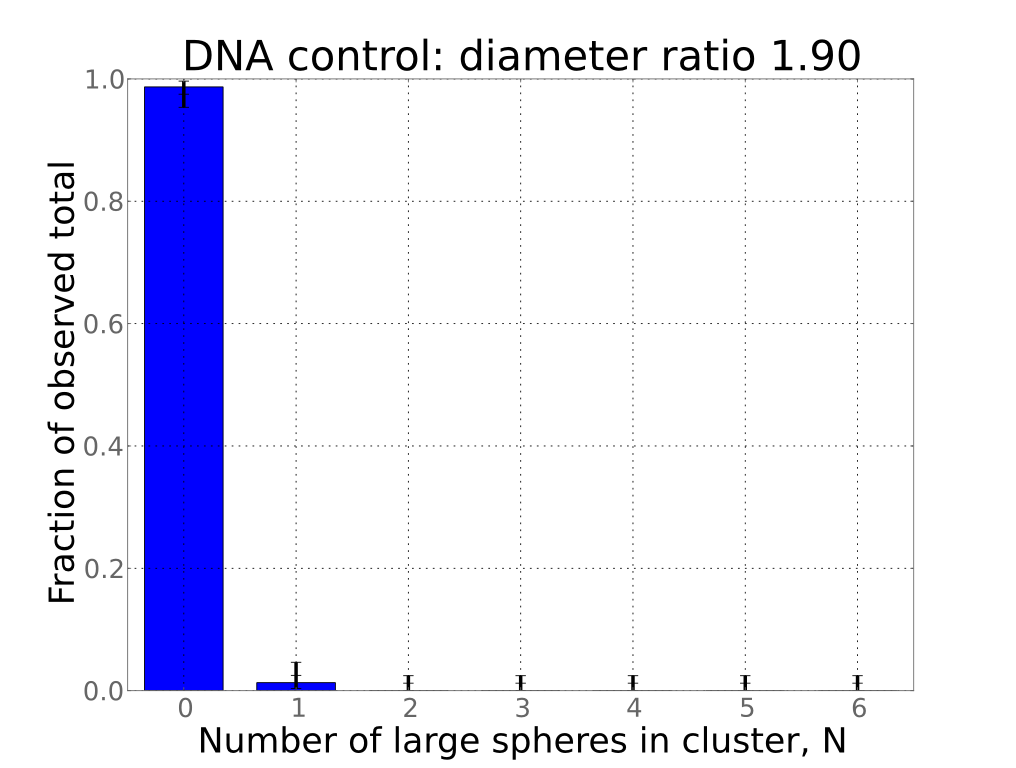
Figure 6: Cluster size distribution in a mixture of $0.97\text{\,}\mathrm{\SIUnitSymbolMicro m}$ non-fluorescent particles and $0.51\text{\,}\mathrm{\SIUnitSymbolMicro m}$ fluorescent particles in a $100:1$ number ratio, coated with the same non-self-complementary DNA sequence (A).

III Measurement of cluster size distribution

To measure the distribution of cluster sizes of a particular mixture, we placed a $5\text{\,}\mathrm{\SIUnitSymbolMicro L}$, 0.1% w/v sample between two cover slips and then sealed it at the edges with UV-curable epoxy (Norland Optical Adhesive 61). We observed each sample under differential interference contrast with a 100X oil-immersion objective on a Nikon Eclipse TE2000-E inverted microscope. We used fluorescence to identify the small spheres.

The distribution was obtained by counting the number of clusters at each $N$. $N=0$ is a small sphere without any large spheres adsorbed, $N=1$ a small sphere attached to a single large sphere, etc. We also counted clusters containing multiple small spheres and clusters formed through non-specific aggregation. The number of such clusters is small compared to the total number of clusters counted. Thus, we do not include these in the histograms.

Our counting procedure is designed to avoid errors from double counting. We begin by counting clusters in the field of view (FOV) on the microscope, scanning through $z$ to find clusters that may initially be out of focus. The Brownian motion of each cluster eventually brings all particles into view. We can therefore determine the number of large and small spheres in each cluster through direct observation. Once we have recorded all clusters in the FOV, we translate the FOV to another part of the sample located more than one FOV away. We repeat this process to build up the histogram, rastering the FOV over the sample. We count more than 60 clusters at each size ratio and more than 120 clusters at size ratios greater than $2$. The entire histogram for a given mixture is recorded in one session on the microscope.

IV Algorithm for simulating random sphere parking

We simulate the cluster distribution using an algorithm based on Monte Carlo trials. These consist of two stages:

Coarse stage

We repeatedly try to insert a disc of radius $r=R_{\mathrm{big}}/(R_{\mathrm{big}}+R_{\mathrm{small}})$ on the surface of the unit sphere. The center of the disc is randomly and uniformly distributed on the sphere. If the disc overlaps any discs that are already “parked”, we reject it; otherwise we add it to the list of parked discs. After a fixed number of consecutive rejections, (typically $N_{\text{coarse}}=10^{4}$), we switch to the fine stage.

Fine stage

We compute the remaining regions of possible insertion, and then try to insert an additional disc. We choose the center of the disc randomly and uniformly from these regions.

To find the regions of possible insertion, we first compute the arcs that form their boundaries: Given a central disc of radius $r$, neighboring disc centers must lie on or outside a concentric circle of radius $2r$. We erase arcs that lie in the interior of the concentric circles of radius $2r$ about each neighboring disc. If the central circle contains any unerased arcs, these are added to our roster of arcs.

We do this for each parked disc center, and then stitch together the remaining arcs to form the regions to which another disc center could be added. To find the area of each region, we inscribe the region in a circumcircle and use a Monte-Carlo integration method to determine the ratio of the area of the region to the area of its circumcircle.

The algorithm terminates when the list of remaining arcs in the fine stage is empty, at which point the final number of inserted discs is recorded.

V Calculating bounds on cluster size distribution

The upper and lower bounds $N_{\max}$ and $N_{\min}$ on the cluster size distribution can be calculated from spherical codes Sloane et al. (2011) corresponding to known solutions to the problems of spherical packings ($N_{\max}$) and spherical coverings ($N_{\min}$). Spherical packings are arrangements of $N$ points on a unit sphere that maximize the smallest distance between any two of them Conway and Sloane (1993); Sloane et al. (2011). For a given $\alpha$ we determine $N_{\max}(\alpha)$ by looking up the spherical packing Sloane et al. (2011) with the largest $N$ for which the minimal distance between points is at least $2\alpha/(1+\alpha)$. Our calculation of $N_{\min}(\alpha)$ is more involved, as explained below.

V.1 Connection between spherical covering and minimum parking

Here we verify that the best known coverings are also optimal solutions to the minimum parking problem. For a given configuration of $n$ “parked” points on a unit sphere, let the covering radius be the maximum distance between any point on the sphere to the nearest parked point. Let the packing radius be (half) the minimum of the pairwise distances between the parked points. If the parked points represent centers of circles with some radius $r$, it is impossible to add another circle without overlapping a parked one if and only if the covering radius is less than $2r$. The circles that are already parked do not overlap provided that the packing radius is greater than $r$. Therefore, if we are given an optimal solution to the covering problem, that is, one that minimizes the covering radius for a given $n$, it will also be the optimal minimal parking configuration if the covering radius is less than 2 times the packing radius.

We manually verify that the best known coverings satisfy this constraint for $n=4,\ldots,130$ by calculating the packing radius for each optimal known covering, obtained from ref. Sloane et al. (2011). Table LABEL:tbl:coverings shows the covering radius, packing radius, and difference (in degrees). The difference is always positive, confirming our statement.

Table 7: Packing and covering radii for different cluster sizes $n$, measured in degrees, and the differences between them. Because the differences are always positive, we conclude that the optimal covering configuration is also the optimal minimal parking configuration, at least for $N\in\{4,\dots,130\}$.

n	2 * packing radius	covering radius	2*(packing radius) - (covering radius)
4	109.47	70.53	38.94
5	90.00	63.43	26.57
6	90.00	54.74	35.26
7	72.00	51.03	20.97
8	61.76	48.14	13.62
9	68.97	45.88	23.09
10	65.53	42.31	23.22
11	50.65	41.43	9.22
12	63.43	37.38	26.06
13	46.23	37.07	9.16
14	52.58	34.94	17.64
15	45.67	34.04	11.63
16	50.48	32.90	17.58
17	41.63	32.09	9.54
18	45.53	31.01	14.51
19	40.73	30.37	10.36
20	40.01	29.62	10.39
21	39.45	28.82	10.62
22	40.70	27.81	12.89
23	38.99	27.48	11.51
24	36.67	26.81	9.86
25	36.75	26.33	10.42
26	35.12	25.84	9.27
27	38.06	25.25	12.81
28	35.87	24.66	11.21
29	33.86	24.37	9.50
30	31.18	23.88	7.30
31	29.94	23.61	6.33
32	37.38	22.69	14.69
33	26.61	22.59	4.02
34	30.82	22.33	8.49
35	27.98	22.07	5.90
36	28.78	21.70	7.08
37	31.22	21.31	9.91
38	30.31	21.07	9.24
39	30.73	20.85	9.87
40	30.13	20.47	9.66
41	27.71	20.32	7.39
42	28.34	20.05	8.29
43	27.27	19.84	7.43
44	26.36	19.64	6.72
45	25.15	19.42	5.73
46	29.11	19.16	9.96
47	25.38	18.99	6.38
48	27.70	18.69	9.01
49	24.93	18.59	6.33
50	28.01	18.30	9.71
51	24.30	18.20	6.10
52	24.24	18.05	6.19
53	22.56	17.88	4.68
54	25.58	17.68	7.90
55	24.06	17.52	6.54
56	24.89	17.35	7.54
57	23.98	17.18	6.80
58	23.72	17.02	6.70
59	23.69	16.90	6.79
60	24.67	16.77	7.90
61	20.50	16.64	3.86
62	20.43	16.49	3.94
63	21.60	16.37	5.23
64	21.34	16.19	5.15
65	20.78	16.11	4.66
66	21.61	15.96	5.66
67	21.32	15.86	5.46
68	21.74	15.72	6.02
69	20.41	15.60	4.82
70	21.47	15.50	5.98
71	21.46	15.39	6.07
72	23.06	15.14	7.92
73	17.51	15.12	2.39
74	17.95	15.03	2.92
75	20.02	14.95	5.07
76	19.08	14.85	4.23
77	22.03	14.74	7.29
78	19.14	14.66	4.49
79	19.77	14.56	5.21
80	19.94	14.45	5.49
81	19.07	14.38	4.69
82	20.40	14.29	6.11
83	17.08	14.22	2.86
84	19.93	14.12	5.81
85	19.92	14.05	5.88
86	19.89	13.96	5.93
87	18.70	13.88	4.81
88	19.80	13.79	6.01
89	19.76	13.71	6.05
90	19.83	13.62	6.21
91	17.18	13.56	3.62
92	17.83	13.49	4.34
93	18.75	13.43	5.32
94	19.15	13.35	5.81
95	18.54	13.29	5.25
96	19.21	13.21	6.00
97	18.38	13.14	5.24
98	18.99	13.06	5.93
99	19.06	13.00	6.06
100	18.58	12.94	5.64
101	18.67	12.87	5.80
102	17.63	12.81	4.82
103	17.51	12.74	4.77
104	18.49	12.67	5.82
105	18.94	12.62	6.32
106	17.66	12.56	5.10
107	18.62	12.50	6.13
108	18.10	12.43	5.67
109	18.23	12.38	5.85
110	18.40	12.30	6.10
111	18.70	12.25	6.45
112	18.71	12.19	6.52
113	18.28	12.15	6.14
114	16.87	12.10	4.78
115	17.42	12.05	5.37
116	16.27	11.99	4.28
117	17.67	11.94	5.73
118	17.71	11.89	5.83
119	17.09	11.84	5.25
120	17.25	11.79	5.47
121	17.56	11.73	5.83
122	17.70	11.68	6.02
123	14.38	11.64	2.74
124	14.14	11.59	2.55
125	17.38	11.54	5.84
126	17.07	11.49	5.58
127	16.54	11.45	5.09
128	16.50	11.41	5.09
129	16.98	11.36	5.62
130	16.95	11.32	5.63

References

- Kelton et al. (2003) K. F. Kelton, G. W. Lee, A. K. Gangopadhyay, R. W. Hyers, T. J. Rathz, J. R. Rogers, M. B. Robinson, and D. S. Robinson, Phys. Rev. Lett. 90, 195504 (2003).
- Manoharan et al. (2003) V. N. Manoharan, M. T. Elsesser, and D. J. Pine, Science 301, 483 (2003).
- Gasser et al. (2001) U. Gasser, E. R. Weeks, A. Schofield, P. N. Pusey, and D. A. Weitz, Science 292, 258 (2001).
- Arkus et al. (2009) N. Arkus, V. N. Manoharan, and M. P. Brenner, Phys. Rev. Lett. 103, 118303 (2009).
- Hoy and O’Hern (2010) R. S. Hoy and C. S. O’Hern, Phys. Rev. Lett. 105, 068001 (2010).
- Meng et al. (2010) G. Meng, N. Arkus, M. P. Brenner, and V. N. Manoharan, Science 327, 560 (2010).
- Yunker et al. (2011) P. J. Yunker, K. Chen, Z. Zhang, W. G. Ellenbroek, A. J. Liu, and A. G. Yodh, Phys. Rev. E 83, 011403 (2011).
- Soto et al. (2002) C. M. Soto, A. Srinivasan, and B. R. Ratna, J. Am. Chem. Soc. 124, 8508 (2002).
- Urzhumov et al. (2007) Y. A. Urzhumov, G. Shvets, J. A. Fan, F. Capasso, D. Brandl, and P. Nordlander, Opt. Express 15, 14129 (2007).
- Alù and Engheta (2009) A. Alù and N. Engheta, Opt. Express 17, 5723 (2009).
- Fan et al. (2010) J. A. Fan, C. Wu, K. Bao, J. Bao, R. Bardhan, N. J. Halas, V. N. Manoharan, P. Nordlander, G. Shvets, and F. Capasso, Science 328, 1135 (2010).
- Melnyk et al. (1977) T. W. Melnyk, O. Knop, and W. R. Smith, Can. J. Chem. 55, 1745 (1977).
- Conway and Sloane (1993) J. H. Conway and N. J. A. Sloane, Sphere Packings, Lattices and Groups (Springer-Verlag, New York, 1993).
- Phillips et al. (2012) C. L. Phillips, E. Jankowski, M. Marval, and S. C. Glotzer, Phys. Rev. E 86, 041124 (2012).
- Egami (1997) T. Egami, Materials Science and Engineering: A 226–228, 261 (1997).
- Miracle (2004) D. B. Miracle, Nat. Mat. 3, 697 (2004).
- Weitz and Oliveria (1984) D. A. Weitz and M. Oliveria, Phys. Rev. Lett. 52, 1433 (1984).
- Lin et al. (1989) M. Y. Lin, H. M. Lindsay, D. A. Weitz, R. C. Ball, R. Klein, and P. Meakin, Nature 339, 360 (1989).
- Note (1) See Supplementary Information at end of manuscript for additional details.
- Miracle et al. (2003) D. B. Miracle, W. S. Sanders, and O. N. Senkov, Phil. Mag. 83, 2409 (2003).
- Dreyfus et al. (2009) R. Dreyfus, M. E. Leunissen, R. Sha, A. V. Tkachenko, N. C. Seeman, D. J. Pine, and P. M. Chaikin, Phys. Rev. Lett. 102, 048301 (2009).
- Dreyfus et al. (2010) R. Dreyfus, M. E. Leunissen, R. Sha, A. Tkachenko, N. C. Seeman, D. J. Pine, and P. M. Chaikin, Phys. Rev. E 81, 041404 (2010).
- Mansfield et al. (1996) M. L. Mansfield, L. Rakesh, and D. A. Tomalia, J. Chem. Phys. 105, 3245 (1996).
- Rosen et al. (1986) L. A. Rosen, N. A. Seaton, and E. D. Glandt, J. Chem. Phys. 85, 7359 (1986).
- Wouterse et al. (2005) A. Wouterse, M. Plapp, and A. P. Philipse, J. Chem. Phys. 123 (2005).
- Talbot et al. (2000) J. Talbot, G. Tarjus, P. R. V. Tassel, and P. Viot, Colloids and Surfaces A: Physicochem. Eng. Aspects 165, 287 (2000).
- Sloane et al. (2011) N. J. A. Sloane, R. H. Hardin, and W. D. Smith, “Tables of spherical codes,” Published electronically at www.research.att.com/njas/packings/ (2011).
- He et al. (1999) D. He, N. N. Ekere, and L. Cai, Phys. Rev. E 60, 7098 (1999).
- Lyon et al. (2004) L. A. Lyon, J. D. Debord, S. B. Debord, C. D. Jones, J. G. McGrath, and M. J. Serpe, J. Phys. Chem. B 108, 19099 (2004).
- Wang et al. (2010) Y. Wang, G. Chen, M. Yang, G. Silber, S. Xing, L. H. Tan, F. Wang, Y. Feng, X. Liu, S. Li, and H. Chen, Nat. Commun. 1 (2010).