Constraints and vibrations in static packings of ellipsoidal particles

Abstract

We numerically investigate the mechanical properties of static packings of ellipsoidal particles in 2D and 3D over a range of aspect ratio and compression $\Delta\phi$. While amorphous packings of spherical particles at jamming onset ($\Delta\phi=0$) are isostatic and possess the minimum contact number $z_{\rm iso}$ required for them to be collectively jammed, amorphous packings of ellipsoidal particles generally possess fewer contacts than expected for collective jamming ($z<z_{\rm iso}$) from naive counting arguments, which assume that all contacts give rise to linearly independent constraints on interparticle separations. To understand this behavior, we decompose the dynamical matrix $M=H-S$ for static packings of ellipsoidal particles into two important components: the stiffness $H$ and stress $S$ matrices. We find that the stiffness matrix possesses $N(z_{\rm iso}-z)$ eigenmodes ${\hat{e}}_{0}$ with zero eigenvalues even at finite compression, where $N$ is the number of particles. In addition, these modes ${\hat{e}}_{0}$ are nearly eigenvectors of the dynamical matrix with eigenvalues that scale as $\Delta\phi$, and thus finite compression stabilizes packings of ellipsoidal particles. At jamming onset, the harmonic response of static packings of ellipsoidal particles vanishes, and the total potential energy scales as $\delta^{4}$ for perturbations by amplitude $\delta$ along these ‘quartic’ modes, ${\hat{e}}_{0}$. These findings illustrate the significant differences between static packings of spherical and ellipsoidal particles.

I Introduction

There have been many experimental scott ; bernal ; gao2 , computational berryman ; torquato_prl ; OHern2003 , and theoretical parisi ; berthier studies of the structural and mechanical properties of disordered static packings of frictionless disks in 2D and spheres in 3D. In these systems, counting arguments, which assume that all particle contacts give rise to linearly independent impenetrability constraints on the particle positions, predict that the minimum number of contacts required for the system to be collectively jammed is $N_{c}\geq N_{c}^{\rm min}=N_{\rm dof}+1$, where $N_{\rm dof}=Nd$ for fixed boundary conditions and $N_{\rm dof}=Nd-d$ for periodic boundary conditions torquato ; witten , where $d$ is the spatial dimension and $N$ is the number of particles rattlers . The additional contact is required because contacts between hard particles provide only inequality constraints on particle separations torquato . In the large-system limit, this relation for the minimum number of contacts reduces to $z\geq z_{\rm iso}$, where $z=2N_{c}/N$ is the average contact number. Disordered packings of frictionless spheres are typically isostatic at jamming onset with $z=z_{\rm iso}$, and possess the minimal number of contacts required to be collectively jammed torquato . Further, it has been shown in numerical simulations that collectively jammed hard-sphere packings correspond to mechanically stable soft-sphere packings in the limit of vanishing particle overlaps OHern2003 ; makse ; apphys .

In contrast, several numerical torquato_ellipse ; Mailman ; zeravcic ; delaney and experimental studies chaikin_prl ; chaikin_science have found that disordered packings of ellipsoidal particles possess fewer contacts ($z<z_{\rm iso}$) than predicted by naive counting arguments, which assume that all contacts give rise to linearly independent constraints on the interparticle separations. Despite this, these packings were found to be mechanically stable (MS) torquato_ellipse ; Mailman .

In a recent manuscript torquato_ellipse by Donev, et al., the authors explained this apparent contradiction—that static packings of ellipsoidal particles are mechanically stable, yet possess $z<z_{\rm iso}$. The main points of the argument are included here. The set of $N_{c}$ interparticle contacts imposes $N_{c}$ constraints, $f_{ij}=1-r_{ij}/\sigma_{ij}\leq 0$, where $r_{ij}$ is the center-to-center separation and $\sigma_{ij}$ is the contact distance along ${\hat{r}}_{ij}$ between particles $i$ and $j$. In disordered MS sphere packings with $z=z_{\rm iso}$, each of the $N_{c}$ interparticle contacts represents a linearly independent constraint. In contrast, some of the $N_{c}$ contacts for MS packings of ellipsoidal particles give rise to linearly dependent constraints. Linearly dependent constraints do not block the degrees of freedom that appear in the constraint equations for sphere packings, whereas they can block multiple degrees of freedom in packings of ellipsoidal particles because they have convex particle shape with a varying radius of curvature torquato_ellipse .

For static packings of spherical particles, interparticle contacts give rise to only “convex” constraints (Fig. 1 (a)), while contacts can yield “convex” or “concave” constraints in packings of ellipsoidal particles (Figs. 1 (a) and (b)). Note that the distinction between convex and concave constraints is different than the distinction between convex and concave particles. For example, ellipsoids have a convex particle shape, but static ellipsoid packings can possess concave interparticle constraints.

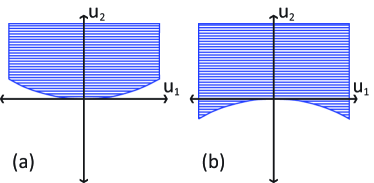
Figure 1: Schematic diagram that illustrates locally (a) convex (positive radius of curvature) and (b) concave (negative radius of curvature) interparticle constraints in packings of hard ellipsoidal particles. Inaccessible regions (with $f_{ij}>0$) are shaded blue. The axes labeled $u_{1}$ and $u_{2}$ indicate two representative orthogonal directions in configuration space.

In jammed packings of ellipsoidal particles, there are $N(z_{\rm iso}-z)$ special directions $\hat{e}_{0}$ in configuration space along which perturbations give rise to interparticle overlaps that scale quadratically with the perturbation amplitude, $f_{ij}\sim\delta^{2}$ torquato_ellipse ; Mailman . Displacements in all other directions yield overlaps that scale linearly with $\delta$, $f_{ij}\sim\delta$, as found for jammed sphere packings. This novel scaling behavior for packings of ellipsoidal particles can be explained by decomposing the dynamical matrix $M=H-S$ for these packings into two important components: the stiffness matrix $H$ that contains all second-order derivatives of the total potential energy $V$ with respect to the configurational degrees of freedom, and the stress matrix $S$ that includes all first-order derivatives of $V$ with respect to the particle coordinates. The directions $\hat{e}_{0}$ are the eigenvectors of the stiffness matrix $H$ with zero eigenvalues.

For static packings of ellipsoidal particles at the jamming threshold ($\Delta\phi=0$) that interact via purely repulsive linear spring potentials (i.e. $V\sim f_{ij}^{2}$), we find that the total potential energy increases quartically when the system is perturbed by $\delta$ along the $\hat{e}_{0}$ directions, $V\propto c\delta^{4}$, where the constant $c>0$. Also, at the jamming threshold, the stress matrix $S=0$ and zero modes of the stiffness matrix are zero modes of the dynamical matrix.

In this manuscript, we will investigate how the mechanical stability of packings of ellipsoidal particles is modified at finite compression ($\Delta\phi>0$). For example, when a system at finite $\Delta\phi$ is perturbed by amplitude $\delta$ along $\hat{e}_{0}$, do quadratic terms in $\delta$ arise in the total potential energy or do the contributions remain zero to second order? If quadratic terms are present, do they stabilize or destabilize the packings, and how do the lowest frequency modes of the dynamical matrix scale with $\Delta\phi$ and aspect ratio?

We find a number of key results for static packings of ellipsoidal particles at finite compression ($\Delta\phi>0$) including: 1) Packings of ellipsoidal particles generically satisfy $z<z_{\rm iso}$ Mailman ; zeravcic ; torquato_ellipse ; delaney ; 2) The stiffness matrix $H$ possesses $N(z_{\rm iso}-z)$ eigenmodes ${\hat{e}}_{0}$ with zero eigenvalues even at finite compression $(\Delta\phi>0)$; and 3) The modes ${\hat{e}}_{0}$ are nearly eigenvectors of the dynamical matrix (and the stress matrix $-S$) with eigenvalues that scale as $c\Delta\phi$, with $c>0$, and thus finite compression stabilizes packings of ellipsoidal particles Mailman . In contrast, for static packings of spherical particles, the stiffness matrix contributions to the dynamical matrix stabilize all modes near jamming onset. At jamming onset ($\Delta\phi=0$), the harmonic response of packings of ellipsoidal particles vanishes, and the total potential energy scales as $\delta^{4}$ for perturbations by amplitude $\delta$ along these ‘quartic’ modes, ${\hat{e}}_{0}$. Our findings illustrate the significant differences between amorphous packings of spherical and ellipsoidal particles.

The remainder of the manuscript will be organized as follows. In Sec. II, we describe the numerical methods that we employed to measure interparticle overlaps, generate static packings, and assess the mechanical stability of packings of ellipsoidal particles. In Sec. III, we describe results from measurements of the density of vibrational modes in the harmonic approximation, the decomposition of the dynamical matrix eigenvalues into contributions from the stiffness and stress matrices, and the relative contributions of the translational and rotational degrees of freedom to the vibrational modes as a function of overcompression and aspect ratio using several packing-generation protocols. In Sec. IV, we summarize our conclusions and provide promising directions for future research. We also include two appendices. In Appendix A, we show that the formation of new interparticle contacts affects the scaling behavior of the potential energy with the amplitude of small perturbations along eigenmodes of the dynamical matrix. In Appendix B, we provide analytical expressions for the elements of the dynamical matrix for ellipse-shaped particles in 2D that interact via a purely repulsive linear spring potential.

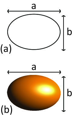
Figure 2: We focus on (a) ellipses in 2D with aspect ratio $\alpha=a/b$ defined as the ratio of the major to minor axis and (b) prolate ellipsoids in 3D where $\alpha$ is the ratio of the polar to equatorial lengths.

II Methods

In this section, we describe the computational methods employed to generate static packings of convex, anisotropic particles, i.e. ellipses in 2D and prolate ellipsoids in 3D with aspect ratio $\alpha=a/b$ of the major to minor axes (Fig. 2), and analyze their mechanical properties. To inhibit ordering in 2D, we studied bidisperse mixtures (2-to-1 relative number density), where the ratio of the major (and minor) axes of the large and small particles is $a_{l}/a_{s}=b_{l}/b_{s}=1.4$. In 3D, we focused on a monodisperse size distribution of prolate ellipsoids. We employed periodic boundaries conditions in unit square (2D) and cubic (3D) cells and studied systems sizes in the range from $N=30$ to $960$ particles to address finite-size effects.

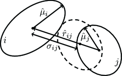
Figure 3: Definition of the contact distance $\sigma_{ij}$ for ellipsoidal particles $i$ and $j$ with unit vectors ${\hat{\mu}}_{i}$ and ${\hat{\mu}}_{j}$ that characterize the orientations of their major axes. $\sigma_{ij}$ is the center-to-center separation at which ellipsoidal particles first touch when they are brought together along ${\hat{r}}_{ij}$ at fixed orientation.

II.1 Contact distance

In both 2D and 3D, we assume that particles interact via the following pairwise, purely repulsive linear spring potential

$$V(r_{ij})=\begin{cases}\frac{\epsilon}{2}\left(1-\frac{r_{ij}}{\sigma_{ij}}\right)^{2}&r_{ij}\leq\sigma_{ij}\\ 0&r_{ij}>\sigma_{ij},\end{cases}$$ (1)

where $\epsilon$ is the characteristic energy of the interaction, $r_{ij}$ is the center-to-center separation between particles $i$ and $j$, and $\sigma_{ij}$ is the orientation-dependent center-to-center separation at which particles $i$ and $j$ come into contact as shown in Fig. 3. Below, energies, lengths, and time scales will be expressed in units of $\epsilon$, $l=\sqrt{I/m}$, and $l\sqrt{m/\epsilon}$, respectively, where $m$ and $I$ are the mass and moment of inertia of the ellipsoidal particles.

Perram and Wertheim developed an efficient method for calculating the exact contact distance between ellipsoidal particles with any aspect ratio and size distribution in 2D and 3D Perram . In their formulation, the contact distance is obtained from

$$\sigma_{ij} = \min_{\lambda}\sigma_{ij}(\lambda),$$ (2)

$$\sigma_{ij}(\lambda) = \frac{\sigma^{0}_{ij}(\lambda)}{\sqrt{1-\frac{\chi(\lambda)}{2}\displaystyle\sum_{\pm}\frac{(\beta(\lambda)\hat{r}_{ij}\cdot\hat{\mu}_{i}\pm\beta(\lambda)^{-1}\hat{r}_{ij}\cdot\hat{\mu}_{j})^{2}}{1\pm\chi(\lambda)\hat{\mu}_{i}\cdot\hat{\mu}_{j}}}},$$

$$\sigma_{ij}^{0}(\lambda) = \frac{1}{2}\sqrt{\frac{b_{i}^{2}}{\lambda}+\frac{b_{j}^{2}}{1-\lambda}},$$

$$\chi(\lambda) = \left(\frac{\left(a_{i}^{2}-b_{i}^{2}\right)\left(a_{j}^{2}-b_{j}^{2}\right)}{\left(a_{j}^{2}+\frac{1-\lambda}{\lambda}b_{i}^{2}\right)\left(a_{i}^{2}+\frac{\lambda}{1-\lambda}b_{j}^{2}\right)}\right)^{1/2},$$

$$\beta(\lambda) = \left(\frac{\left(a_{i}^{2}-b_{i}^{2}\right)\left(a_{j}^{2}+\frac{1-\lambda}{\lambda}b_{i}^{2}\right)}{\left(a_{j}^{2}-b_{j}^{2}\right)\left(a_{i}^{2}+\frac{\lambda}{1-\lambda}b_{j}^{2}\right)}\right)^{1/4}.$$

The approximation $\sigma^{a}_{ij}=\sigma_{ij}(\lambda=1/2)$ is equivalent to the commonly used Gay-Berne approximation for the contact distance Perram1996 ; Cleaver . The accuracy of the Gay-Berne approximation depends on the relative orientation of the two ellipsoidal particles, and in general is more accurate for monodisperse systems. For example, in Fig. 4, we show $\sigma_{ij}^{a}$ for several relative orientations of both monodisperse and bidisperse systems. The relative deviation from the true contact distance can be as large as $e\sim 10\%$ for $a_{j}/a_{i}=1.4$ and $\alpha=2$. Thus, the Gay-Berne approximation should be used with caution when studying polydisperse packings of ellipsoidal particles. For monodisperse ellipses with $\alpha=2$, $0\%<e<5\%$. We find similar results for 3D systems. Unless stated otherwise, we employ the exact expression for contact distance, and thus $\sigma_{ij}=\sigma_{ij}(\lambda_{\rm min})$, $\beta=\beta(\lambda_{\rm min})$, $\chi=\chi(\lambda_{\rm min})$, and $\sigma_{ij}^{0}=\sigma_{ij}^{0}(\lambda_{\rm min})$, where $\lambda_{\rm min}$ is the minimum obtained from Eq. 2.

Figure 4: Ellipses with $\alpha=2$ positioned at the Gay-Berne contact distance $\sigma^{a}_{ij}$. For two ellipses with the same size, the (a) end-to-end configuration is exact, while the (b) side-to-end configuration has a $5\%$ relative error. For two ellipses with $a_{j}/a_{i}=1.4$, the (c) end-to-end configuration has a relative error of $1\%$, while the (d) side-to-end configuration has a relative error of $10\%$.

II.2 Packing generation protocol

We employ a frequently used isotropic compression method for soft, purely repulsive particles xu ; gao to generate static packings of ellipsoidal particles at jamming onset ($\Delta\phi=0$). Static packings at jamming onset are characterized by infinitesimal but nonzero total potential energy and pressure. This isotropic compression method consists of the following steps. We begin by randomly placing particles at low packing fraction ($\phi_{0}=0.2$) with random orientations and zero velocities in the simulation cell. We successively compress the system by small packing fraction increments $\delta\phi=10^{-3}$, with each compression followed by conjugate gradient (CG) energy minimization until the total potential energy per particle drops below a small threshold, $V/N\leq V_{\rm tol}=10^{-16}$, or the total potential energy per particle between successive iterations of the minimization routine is $(V_{t+1}-V_{t})/V_{t}\leq V_{\rm tol}$. The algorithm switches from compression to decompression if the minimized energy is greater than $2V_{\rm tol}$. Each time the algorithm toggles from compression to decompression or vice versa, the packing fraction increment is halved.

The packing-generation algorithm is terminated when the total potential energy per particle satisfies $V_{\rm tol}<V/N<2V_{\rm tol}$. Thus, using this method we can locate the jammed packing fraction $\phi_{J}$ and particle positions at jamming onset for each initial condition to within $10^{-8}$. After jamming onset is identified, we also generate configurations at specified $\Delta\phi=\phi-\phi_{J}$ over six orders of magnitude from $10^{-8}$ to $10^{-2}$ by applying a prescribed set of compressions with each followed by energy minimization.

To determine whether the accuracy of the energy minimization algorithm affects our results (see Sec. III.4), we calculate the eigenvalues of the dynamical matrix as a function of the total kinetic energy (or deviation from zero in force and torque balance on each particle) at each $\Delta\phi$. To do this, we initialize the system with MS packings from the above packing-generation algorithm and use molecular dynamics (MD) simulations with damping terms proportional to the translational and rotational velocities of the ellipsoidal particles to remove excess kinetic energy from the system foot_md . The damped MD simulations are terminated when the total kinetic energy per particle is below $K/N=K_{\rm tol}$, where $K_{\rm tol}$ is varied from $10^{-16}$ to $10^{-32}$. This provides accuracy in the particle positions of the energy minimized states in the range from $10^{-8}$ to $10^{-16}$.

For the damped MD simulations, we solve Newton’s equations of motion (using fifth-order Gear predictor-corrector methods allen ) for the center of mass position and angles that characterize the orientation of the long axis of the ellipsoidal particles. In 2D, we solve

$$m\frac{d^{2}{\vec{r}}_{i}}{dt^{2}} = \sum_{i>j}{\vec{F}}_{ij}-b_{r}{\vec{v}}_{i}$$ (3)

$$I\frac{d^{2}\theta_{i}}{dt^{2}} = \sum_{i>j}T_{ij}-b_{\theta}{\dot{\theta}}_{i},$$ (4)

where $\theta_{i}$ is the angle the long axis of ellipse $i$ makes with the horizontal axis, ${\vec{v}}_{i}$ is the translational velocity of particle $i$, ${\dot{\theta}}_{i}$ is the rotational speed of particle $i$, $b_{r}$ and $b_{\theta}$ are the damping coefficients for the position and angle degrees of freedom, and the moment of inertia $I=m(a^{2}+b^{2})/4$. The force ${\vec{F}}_{ij}$ on ellipse $i$ arising from an overlap with ellipse $j$ is

$$\vec{F}_{ij} = -F_{ij}\frac{\hat{r}_{ij}-\frac{\partial\ln\sigma_{ij}}{\partial\psi_{ij}}\hat{\psi}_{ij}}{\sqrt{1+\big{(}\frac{\partial\ln\sigma_{ij}}{\partial\psi_{ij}}\big{)}^{2}}},$$ (5)

where

$$F_{ij} = \sqrt{1+\left(\frac{\partial\ln\sigma_{ij}}{\partial\psi_{ij}}\right)^{2}}\left|\frac{\partial V(r_{ij})}{\partial r_{ij}}\right|,$$ (6)

$$\frac{\partial\ln\sigma_{ij}}{\partial\psi_{ij}} = -\frac{\chi}{2}\frac{\sigma_{ij}^{2}}{(\sigma_{ij}^{0})^{2}}\big{[}(\beta^{2}-\chi)\sin\left[2(\psi_{ij}-\theta_{i})\right]+$$ (7)

$$(\beta^{-2}-\chi)\sin\left[2(\psi_{ij}-\theta_{j})\right]\big{]}\times$$

$$\left(1-\chi^{2}\cos^{2}\left[\theta_{i}-\theta_{j}\right]\right)^{-1},$$

$-dV(r_{ij})/dr_{ij}=\sigma^{-1}_{ij}(1-\frac{r_{ij}}{\sigma_{ij}})$ for the purely repulsive linear spring potential in Eq. 1, and $\hat{r}_{ij}$ and $\hat{\psi}_{ij}$ are illustrated in Fig. 5.

To calculate the torque $T_{ij}=[\vec{r_{ij}^{c}}\times\vec{F}_{ij}]\cdot{\hat{z}}$ in Eq. 4, we must identify the point of contact between particles $i$ and $j$,

$$\vec{r}_{ij}^{c} = \frac{b_{i}}{2}\frac{1}{\sqrt{\alpha^{-2}+\tan^{2}\tau_{ij}}}\times$$ (8)

$$\big{[}(\cos\theta_{i}-\sin\theta_{i}\tan\tau_{ij})\hat{x}+$$

$$(\sin\theta_{i}\tan\tau_{ij}+\cos\theta_{i})\hat{y}\big{]},$$

where

$$\tan\tau_{ij} = \alpha^{-2}\frac{\tan(\psi_{ij}-\theta_{i})-\frac{\partial\ln\sigma_{ij}}{\partial\psi_{ij}}}{1+\tan(\psi_{ij}-\theta_{i})\frac{\partial\ln\sigma_{ij}}{\partial\psi_{ij}}}$$ (9)

and $\vec{r}_{ij}^{c}$, $\psi_{ij}$, and $\tau_{ij}$ are depicted in Fig. 5. From Eqs. 5 and 8, we find

$$T_{ij} = -\frac{b_{i}F_{ij}}{2}\times$$ (10)

$$\frac{\big{(}1-\alpha^{-2}\big{)}\tan\tau_{ij}}{\sqrt{\big{(}1+\alpha^{-4}\tan^{2}\tau_{ij}\big{)}\big{(}1+\alpha^{-2}\tan^{2}\tau_{ij}\big{)}}}.$$

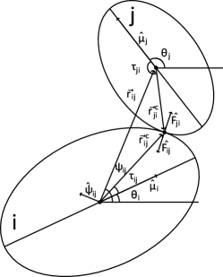
Figure 5: Geometry of two ellipses in contact. The angles $\theta_{i}$ and $\theta_{j}$ characterize the orientation of particles $i$ and $j$ relative to the horizontal axis, i.e. ${\hat{\mu}}_{i}=\cos\theta_{i}{\hat{x}}+\sin\theta_{i}{\hat{y}}$. $\psi_{ij}$ gives the angle between the center-to-center separation vector ${\vec{r}}_{ij}$ and the horizontal axis and ${\hat{\psi}}_{ij}=-\sin\psi_{ij}{\hat{x}}+\cos\psi_{ij}{\hat{y}}$ is the angle unit vector in polar coordinates. The unit vector ${\hat{F}}_{ij}=-{\hat{F}}_{ji}$ points in the direction of the force on particle $i$ due to particle $j$ at the point of contact. ${\vec{r}}^{c}_{ij}$ points from the center of particle $i$ to the point of contact with particle $j$, and $\tau_{ij}$ is the angle between ${\hat{\mu}}_{i}$ and ${\vec{r}}^{c}_{ij}$.

II.3 Dynamical matrix calculation

To investigate the mechanical properties of static packings of ellipsoidal particles, we will calculate the eigenvalues of the dynamical matrix and the resulting density of vibrational modes in the harmonic approximation schreck2011 . The dynamical matrix is defined as

$$M_{kl} = \frac{\partial^{2}V}{\partial u_{k}\partial u_{l}},$$ (11)

where $u_{k}$ (with $k=1,\ldots,d_{f}N$) represent the $d_{f}N$ degrees of freedom in the system and $d_{f}$ is the number of degrees of freedom per particle. In 2D $d_{f}=3$ with ${\vec{u}}=\{x_{1}$,$x_{2}$,$\ldots$,$x_{N}$,$y_{1}$,$y_{2}$,$\ldots$,$y_{N}$,$l_{2}\theta_{1}$,$l_{2}\theta_{2}$,$\ldots$,$l_{2}\theta_{N}$} and in 3D for prolate ellipsoids $d_{f}=5$ with ${\vec{u}}=\{x_{1}$,$x_{2}$,$\ldots$,$x_{N}$,$y_{1}$, $y_{2}$,$\ldots$,$y_{N}$,$z_{1}$,$z_{2}$,$\ldots$,$z_{N}$,$l_{\theta}^{1}\theta_{1}$,$l_{\theta}^{2}\theta_{2}$,$\ldots$,$l_{\theta}^{N}\theta_{N}$,$l_{3}\phi_{1}$,$l_{3}\phi_{2}$,$\ldots$, $l_{3}\phi_{N}$}, where $\theta_{i}$ is the polar angle and $\phi_{i}$ is the azimuthal angle in spherical coordinates, $l_{2}=\sqrt{a^{2}+b^{2}}/2$, $l_{3}=\sqrt{\big{(}a^{2}+b^{2}\big{)}/5}$, and $l_{\theta}^{i}=\sqrt{\big{(}2b^{2}+(a^{2}-b^{2})\sin^{2}\phi_{i}\big{)}/5}$.

The dynamical matrix requires calculations of the first and second derivatives of the total potential energy $V$ with respect to all positional and angular degrees of freedom in the system. The first derivatives of $V$ with respect to the positions of the centers of mass of the particles ${\vec{r}}_{i}$ can be obtained from Eq. 5. In 2D, there is only one first derivative involving angles, $F_{\theta}^{i}=-\partial V(r_{ij})/\partial\theta_{i}$, where

$$F_{\theta}^{i} = \frac{1}{4}\chi\bigg{(}\frac{\sigma_{ij}}{\sigma_{ij}^{0}}\bigg{)}^{2}(2\alpha A(B_{+}+B_{-})+\chi C(B_{+}^{2}-B_{-}^{2})),$$ (12)

$$A = \frac{y_{ij}\cos\theta_{i}-x_{ij}\sin\theta_{i}}{r_{ij}},$$

$$B_{\pm} = \frac{\alpha(x_{ij}\cos\theta_{i}+y_{ij}\sin\theta_{i})\pm\alpha^{-1}(x_{ij}\cos\theta_{j}+y_{ij}\sin\theta_{j})}{(1+\chi\cos[\theta_{i}-\theta_{j}])r_{ij}},$$

$$C = \cos^{2}(\theta_{i}-\theta_{j}).$$

Complete expressions for the matrix elements of the dynamical matrix for ellipses in 2D are provided in Appendix B. In 3D, we calculated the first derivatives of $V$ with respect to the particle coordinates analytically, and then evaluated the second derivatives for the dynamical matrix numerically.

The vibrational frequencies in the harmonic approximation can be obtained from the $Nd_{f}-d$ nontrivial eigenvalues $m_{i}$ of the dynamical matrix, $\omega_{i}=\sqrt{m_{i}/\epsilon}b_{s}$. $d$ of the eigenvalues are zero due to periodic boundary conditions. For all static packings, we have verified that the smallest nontrivial eigenvalue satisfies $m_{\rm min}/N>10^{-10}$.

Below, we will study the density of vibrational frequencies $D(\omega)=(N(\omega+\Delta\omega)-N(\omega))/(N_{\rm dof}\Delta\omega)$ as a function of compression $\Delta\phi$ and aspect ratio $\alpha$, where $N(\omega)$ is the number of vibrational frequencies less than $\omega$. We will also investigate the relative contributions of the translational and rotational degrees of freedom to the nontrivial eigenvectors of the dynamical matrix, ${\hat{m}}_{i}=\{m_{xi}^{j=1},m_{yi}^{j=1},m_{\theta i}^{j=1},\ldots,m_{xi}^{j=N},m_{yi}^{j=N},m_{\theta i}^{j=N}\}$ for ellipses in 2D and ${\hat{m}}_{i}=\{m_{xi}^{j=1},m_{yi}^{j=1},m_{zi}^{j=1},m_{\theta i}^{j=1},m_{\phi i}^{j=1},\ldots,m_{xi}^{j=N},m_{yi}^{j=N},m_{zi}^{j=N},$ $m_{\theta i}^{j=N},m_{\phi i}^{j=N}\}$ for prolate ellipsoids in 3D, where $i$ labels the eigenvector and runs from $1$ to $Nd_{f}-d$. The eigenvectors are normalized such that ${\hat{m}}_{i}^{2}=1$.

II.4 Dynamical matrix decomposition

The dynamical matrix (Eq. 11) can be decomposed into two component matrices $M=H-S$: 1) the stiffness matrix $H$ that includes only second-order derivatives of the total potential energy $V$ with respect to the configurational degrees of freedom and 2) the stress matrix $S$ that includes only first-order derivatives of $V$. The $kl$ elements of $H$ and $S$ are given by

$$H_{kl} = \sum_{i>j}\frac{\partial^{2}V}{\partial(r_{ij}/\sigma_{ij})^{2}}\frac{\partial(r_{ij}/\sigma_{ij})}{\partial u_{k}}\frac{\partial(r_{ij}/\sigma_{ij})}{\partial u_{l}}$$ (13)

$$S_{kl} = -\sum_{i>j}\frac{\partial V}{\partial(r_{ij}/\sigma_{ij})}\frac{\partial^{2}(r_{ij}/\sigma_{ij})}{\partial u_{k}\partial u_{l}},$$ (14)

where the sums are over distinct pairs of overlapping particles $i$ and $j$. Since $\partial^{2}V/\partial(r_{ij}/\sigma_{ij})^{2}=\epsilon$ for the purely repulsive linear spring potential (Eq. 1), the stiffness matrix depends only on the geometry of the packing (i.e. $\partial(r_{ij}/\sigma_{ij})/\partial u_{k})$. Also, at zero compression $\Delta\phi=0$, $S=0$, $M=H$, and only the stiffness matrix contributes to the dynamical matrix. The frequencies associated with the eigenvalues $h_{i}$ of the stiffness matrix (at any $\Delta\phi$) are denoted by $\omega_{hi}=\sqrt{h_{i}/\epsilon}b_{s}$, and the stiffness matrix eigenvectors are normalized such that ${\hat{h}}_{i}^{2}=1$.

II.5 Contact number

When counting the number of interparticle contacts $N_{c}$, we remove all rattler particles (defined as those with fewer than $d+1$ contacts) and do not include the contacts that rattler particles make with non-rattler particles foot_contact . Removing these contacts may cause non-rattler particles to become rattlers, and thus this process is performed recursively. Note that for ellipsoidal particles with $d+1$ contacts, the lines normal to the points (or planes in 3D) of contact must all intersect, otherwise the system is not mechanically stable. The number of contacts per particle is defined as $z=N_{c}/(N-N_{r})$, where $N_{r}$ is the number of rattlers. We find that the number of rattler particles decreases with aspect ratio from approximately $5\%$ of the system at $\alpha=1$ to zero for $\alpha>1.2$ in both 2D and 3D.

III Results

Static packings of ellipsoidal particles at jamming onset typically possess fewer contacts than predicted by isostatic counting arguments torquato_ellipse , $z<z_{\rm iso}$, over a wide range of aspect ratio as shown in Fig. 6. This finding raises a number of important questions. For example, are static packings of ellipsoidal particles mechanically stable at finite $\Delta\phi>0$, i.e. does the dynamical matrix for these systems possess nontrivial zero-frequency modes at $\Delta\phi>0$? In this section, we will show that packings of ellipsoidal particles are indeed mechanically stable (with no nontrivial zero-frequency modes) by calculating the dynamical, stress, and stiffness matrices for these systems as a function of compression $\Delta\phi$, aspect ratio $\alpha$, and packing-generation protocol. Further, we will show that the density of vibrational modes for these systems possesses three characteristic frequency regimes and determine the scaling of these characteristic frequencies with $\Delta\phi$ and $\alpha$.

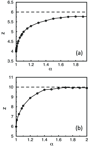
Figure 6: Average contact number $z$ versus aspect ratio $\alpha$ for static packings of (a) bidisperse ellipses in 2D and (b) prolate ellipsoids in 3D at jamming onset. The isostatic values $z_{\rm iso}=6$ (2D) and $10$ (3D) are indicated by dashed lines.

III.1 Density of vibrational frequencies $D(\omega)$

A number of studies have shown that amorphous sphere packings are fragile solids in the sense that the density of vibrational frequencies (in the harmonic approximation) $D(\omega)$ for these systems possesses an excess of low-frequency modes over Debye solids near jamming onset, i.e. a plateau forms and extends to lower frequencies as $\Delta\phi\rightarrow 0$ OHern2003 ; silbert2005 ; wyart . In this work, we will calculate $D(\omega)$ as a function of $\Delta\phi$ and aspect ratio $\alpha$ for amorphous packings of ellipsoidal particles and show that the density of vibrational modes for these systems shows significant qualitative differences from that for spherical particles.

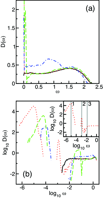
Figure 7: (a) The density of vibrational frequencies $D(\omega)$ for $N=240$ ellipse-shaped particles at $\Delta\phi=10^{-8}$ with aspect ratio $\alpha=1.0$ (solid), $1.001$ (dotted), $1.05$ (dashed), and $2.0$ (dot-dashed). $D(\omega)$ for $\alpha=1$ has been scaled by $2/3$ relative to those with $\alpha>1$ to achieve collapse at low aspect ratios. (b) $D(\omega)$ for the same aspect ratios in (a) on a $\log$-$\log$ scale. The inset illustrates the three characteristic frequencies $\omega_{1}$, $\omega_{2}$, and $\omega_{3}$ in $D(\omega)$ for $\alpha=1.001$.

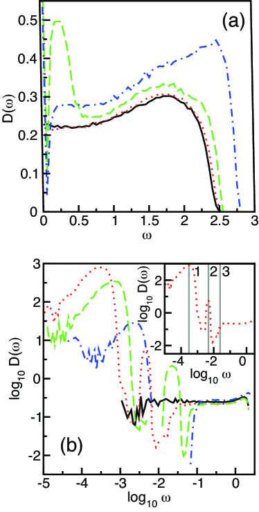
Figure 8: (a) The density of vibrational frequencies $D(\omega)$ for $N=512$ prolate ellipsoids at $\Delta\phi=10^{-6}$ for $\alpha=1.0$ (solid), $1.001$ (dotted), $1.005$ (dashed), and $1.2$ (dot-dashed). $D(\omega)$ for $\alpha=1$ has been scaled by $3/5$ relative to those with $\alpha>1$ to achieve collapse at low aspect ratios. (b) $D(\omega)$ for the same aspect ratios in (a) on a $\log$-$\log$ scale. The inset illustrates the three characteristic frequencies $\omega_{1}$, $\omega_{2}$, and $\omega_{3}$ in $D(\omega)$ for $\alpha=1.001$.

In Figs. 7 (a) and (b), we show $D(\omega)$ on linear and $\log$-$\log$ scales, respectively, for ellipse-shaped particles in 2D at $\Delta\phi=10^{-8}$ over a range of aspect ratios from $\alpha=1$ to $2$. We find several key features in $D(\omega)$: 1) For low aspect ratios $\alpha<1.05$, $D(\omega)$ collapses with that for disks ($\alpha=1$) at intermediate and large frequencies $0.25<\omega<2.25$; 2) For large aspect ratios $\alpha\geq 2$, $D(\omega)$ is qualitatively different for ellipses than for disks over the entire frequency range; and 3) A strong peak near $\omega=0$ and a smaller secondary peak at intermediate frequencies (evident on the log-log scale in Fig. 7 (b)) occur in $D(\omega)$ for $\alpha>1$. Note that at finite compression $\Delta\phi>0$, we do not find any nontrivial zero-frequency modes of the dynamical matrix in static packings of ellipses and ellipsoids. The only zero-frequency modes in these systems correspond to the $d$ constant translations that arise from periodic boundary conditions and zero-frequency modes associated with ‘rattler’ particles with fewer than $d+1$ interparticle contacts.

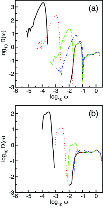
Figure 9: The density of vibrational frequencies $D(\omega)$ for $N=240$ ellipses as a function of compression $\Delta\phi=10^{-7}$ (solid), $10^{-5}$ (dashed), $10^{-3}$ (dotted), and $10^{-2}$ (dot-dashed) for (a) $\alpha=1.05$ and (b) $2$.

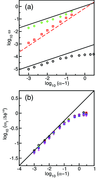
Figure 10: (a) Characteristic frequencies $\omega_{1}$ (circles), $\omega_{2}$ (squares), and $\omega_{3}$ (diamonds) from $D(\omega)$ as a function of aspect ratio $\alpha-1$ for $N=240$ ellipses in 2D at $\Delta\phi=10^{-8}$. The solid (dashed) lines have slope $1/2$ ($1)$. (b) $\omega_{1}/(\Delta\phi)^{1/2}$ for systems with $N=240$ ellipses in 2D at $\Delta\phi=10^{-7}$ (circles), $10^{-6}$ (squares), $10^{-5}$ (diamonds), $10^{-4}$ (upward triangles), $10^{-3}$, (downward triangles), and $10^{-2}$ (crosses). The solid line has slope $1/2$.

To monitor the key features of $D(\omega)$ as a function of $\Delta\phi$ and $\alpha$, we define three characteristic frequencies as shown in the inset to Fig. 7 (b). $\omega_{1}$ and $\omega_{2}$ identify the locations of the small and intermediate frequency peaks in $D(\omega)$, and $\omega_{3}$ marks the onset of the high-frequency plateau regime in $D(\omega)$. For our analysis, we define $\omega_{3}$ as the largest frequency ($<1$) with $D(\omega)<0.15$, which is approximately half of the height of the plateau in $D(\omega)$ at large frequencies. All three characteristic frequencies increase with aspect ratio. Note that we only track $\omega_{2}$ and $\omega_{3}$ for aspect ratios where $\omega_{2}<\omega_{3}$. For example, the intermediate and high-frequency bands characterized by $\omega_{2}$ and $\omega_{3}$ merge for $\alpha\geq 1.2$.

As shown in Fig. 8, $D(\omega)$ for 3D prolate ellipsoids displays similar behavior to that for ellipses in 2D (Fig. 7) for aspect ratios $\alpha<1.5$. For example, $D(\omega)$ for ellipsoids possesses low, intermediate, and high frequency regimes, whose characteristic frequencies $\omega_{1}$, $\omega_{2}$, and $\omega_{3}$ increase with aspect ratio. Note that the intermediate and high-frequency bands $\omega_{2}$ and $\omega_{3}$ merge for $\alpha>1.02$, which occurs at lower aspect ratio than the merging of the bands in 2D. Another significant difference is that in 3D $D(\omega)$ extends to higher frequencies at large aspect ratios ($\alpha\gtrsim 1.2$) than $D(\omega)$ for ellipses.

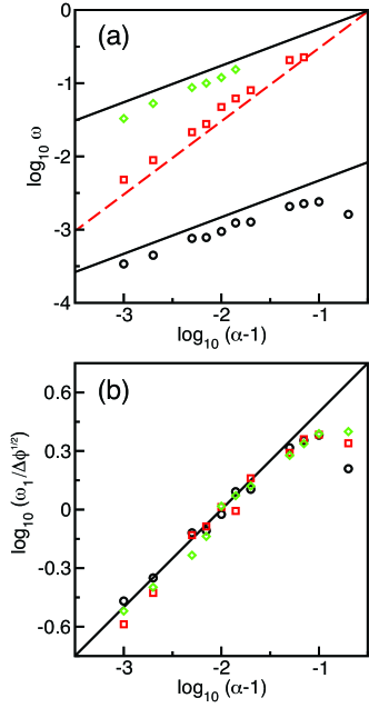
Figure 11: (a) Characteristic frequencies $\omega_{1}$ (circles), $\omega_{2}$ (squares), and $\omega_{3}$ (diamonds) from $D(\omega)$ as a function of aspect ratio $\alpha-1$ for $N=240$ prolate ellipsoids in 3D at $\Delta\phi=10^{-6}$. The solid (dashed) lines have slope $1/2$ ($1)$. (b) $\omega_{1}/(\Delta\phi)^{1/2}$ for systems with $N=240$ prolate ellipsoids at $\Delta\phi=10^{-6}$ (circles), $10^{-5}$ (squares), and $10^{-4}$ (diamonds). The solid line has slope $1/2$.

We note the qualitative similarity between the $D(\omega)$ for $\alpha=1.005$ ellipsoids shown in Fig. 8 (b) and $D(\omega)$ for $\alpha=0.96$ presented in Fig. 1 (c) of Ref. zeravcic for $\omega>10^{-2}$. However, Zeravcic, et al. suggest that there is no weight in $D(\omega)$ for $\omega<10^{-2}$ except at $\omega=0$ for both oblate and prolate ellipsoids, in contrast to our results in Fig. 8.

In Fig. 9, we show the behavior of $D(\omega)$ for ellipse packings as a function of compression $\Delta\phi$ for two aspect ratios, $\alpha=1.05$ and $2$. We find that the low-frequency band (characterized by $\omega_{1})$ depends on $\Delta\phi$, while the intermediate and high frequency bands do not. The intermediate and high frequencies bands do not change significantly until the low-frequency band centered at $\omega_{1}$ merges with them at $\Delta\phi\approx 10^{-3}$ and $\approx 10^{-4}$ for $\alpha=1.05$ and $2$, respectively.

We plot the characteristic frequencies $\omega_{1}$, $\omega_{2}$, and $\omega_{3}$ versus aspect ratio $\alpha-1$ for ellipse packings in Fig. 10 and ellipsoid packings in Fig. 11. The characteristic frequencies obey the following scaling laws over at least two orders of magnitude in $\alpha-1$ and five orders of magnitude in $\Delta\phi$:

$$\omega_{1} \sim (\Delta\phi)^{1/2}(\alpha-1)^{1/2},$$ (15)

$$\omega_{2} \sim (\alpha-1),$$ (16)

$$\omega_{3} \sim (\alpha-1)^{1/2}.$$ (17)

Similar results for the scaling of $\omega_{2}$ and $\omega_{3}$ with $\alpha-1$ were found in Ref. zeravcic . We will refer to the modes in the low-frequency band in $D(\omega)$ (with characteristic frequency $\omega_{1}$) as ‘quartic modes’, and these will be discussed in detail Sec. III.3. The scaling of the quartic mode frequencies with compression, $\omega_{1}\sim(\Delta\phi)^{1/2}$, has important consequences for the linear response behavior of ellipsoidal particles to applied stress Mailman .

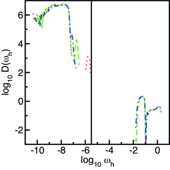
Figure 12: The distribution of frequencies $D(\omega_{h})$ associated with the eigenvalues of the stiffness matrix $H$ for $N=240$ ellipse packings as a function of compression $\Delta\phi=10^{-5}$ (dotted), $10^{-3}$ (dashed), and $10^{-2}$ (dot-dashed) for $\alpha=1.05$. The vertical solid line indicates the ‘zero-frequency’ tolerance $\omega_{\rm tol}$, which is the lowest frequency obtained for the dynamical matrix for packings at $\alpha=1.05$ and the smallest compression ($\Delta\phi=10^{-8}$) in Fig. 7.

III.2 Dynamical Matrix Decomposition

As shown in Fig. 6, static packings of ellipsoidal particles can possess $z<z_{\rm iso}$ over a wide range of aspect ratio, yet as described in Sec. III.1, the dynamical matrix $M$ contains a complete spectrum of $Nd_{f}-d$ nonzero eigenvalues $m_{i}$ near jamming. To investigate this intriguing property, we first calculate the eigenvalues of the stiffness matrix $H$, show that it possesses $N_{z}$ ‘zero’-frequency modes whose number matches the deviation in the contact number from the isostatic value, and then identify the separate contributions from the stiffness and stress matrices to the dynamical matrix eigenvalues.

In Fig. 12, we show the distribution of frequencies $D(\omega_{h})$ associated with the eigenvalues of the stiffness matrix for ellipse packings at $\alpha=1.05$ as a function of compression $\Delta\phi$. We find three striking features in Fig. 12: 1) Many modes of the stiffness matrix exist near and below the zero-frequency threshold (determined by the vibrational frequencies of the dynamical matrix at $\alpha=1.05$ and $\Delta\phi=10^{-8}$), 2) Frequencies that correspond to the low-frequency band characterized by $\omega_{1}$ are absent, and 3) The nonzero frequency modes (with $\omega_{h}>10^{-2}$) do not scale with $\Delta\phi$ as pointed out for the dynamical matrix eigenvalues in Eqs. 16 and 17. Further, we find that the number of zero-frequency modes $N_{z}$ of the stiffness matrix matches the deviation in the number of contacts from the isostatic value ($N_{\rm iso}-N_{c}$) for each $\Delta\phi$ and aspect ratio. Specifically, $N_{z}=N_{\rm iso}-N_{c}$ over the full range of $\Delta\phi$ for $99.96\%$ of the more than $10^{3}$ packings for aspect ratio $\alpha<1.1$ and for $100\%$ of the more than $10^{3}$ packings for $\alpha\geq 1.1$.

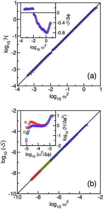
Figure 13: The two contributions to the dynamical matrix eigenvalues, (a) ${\cal H}$ and (b) $-{\cal S}$, plotted versus $\omega^{2}={\cal H}-{\cal S}$ for ellipse packings with $\alpha=1.05$ and $\Delta\phi=10^{-6}$ (circles), $10^{-5}$ (squares), $10^{-4}$ (diamonds), and $10^{-3}$ (triangles). In (a) and (b), the solid lines correspond to ${\cal H}=\omega^{2}$ and ${\cal S}=\omega^{2}$. In the main panel and inset of (a), only modes corresponding the intermediate and high frequency bands are included. In the main panel and inset of (b), only modes corresponding the low frequency band are included. The insets to (a) and (b), which plot $-{\cal S}/(\Delta\phi)^{2}$ versus $\omega^{2}$ and ${\cal H}/(\Delta\phi)^{2}$ versus $\omega^{2}/\Delta\phi$, show the deviations $\omega^{2}-{\cal H}=-{\cal S}\propto\Delta\phi$ for high- and intermediate-frequency modes and $\omega^{2}-(-{\cal S})={\cal H}\propto(\Delta\phi)^{2}$ for low-frequency modes.

In Fig. 13, we calculate the projection of the dynamical matrix eigenvectors ${\hat{m}}_{i}$ onto the stiffness and stress matrices, ${\cal H}={\hat{m}}_{i}^{\dagger}H{\hat{m}}_{i}$ and ${\cal S}={\hat{m}}_{i}^{\dagger}S{\hat{m}}_{i}$, where ${\hat{m}}_{i}^{\dagger}$ is the transpose of ${\hat{m}}_{i}$ and $\omega_{i}^{2}={\hat{m}}_{i}^{\dagger}M{\hat{m}}_{i}={\cal H}-{\cal S}$. Fig. 13 (a) shows that for large eigenvalues $\omega_{i}^{2}$ of the dynamical matrix (i.e. within the intermediate and high frequency bands characterized by $\omega_{2}$ and $\omega_{3}$ in Fig. 7), the eigenvalues of the stiffness and dynamical matrices are approximately the same, ${\cal H}\approx\omega_{i}^{2}$. The deviation $\omega_{i}^{2}-{\cal H}=-{\cal S}$, shown in the inset to Fig. 13 (a), scales linearly with $\Delta\phi$. Thus, we find that the intermediate and high frequency modes for packings of ellipsoidal particles are stabilized by the stiffness matrix $H$.

In the main panel of Fig. 13 (b), we show that for frequencies in the lowest frequency band (characterized by $\omega_{1}$) the eigenvalues of the stress and dynamical matrices are approximately the same, $-{\cal S}\approx\omega_{i}^{2}$. In the inset to Fig. 13 (b), we show that the deviation $\omega_{i}^{2}-({-\cal S})={\cal H}$ scales as $(\Delta\phi)^{2}$. Thus, we find that the lowest frequency modes for packings of ellipsoidal particles are stabilized by the stress matrix $-S$ over a wide range of compression $\Delta\phi$. Similar results were found previously for packings of hard ellipsoidal particles torquato_ellipse . In contrast, for static packings of spherical particles, the stress matrix contributions to the dynamical matrix are destabilizing with $-{\cal S}<0$ for all frequencies near jamming, and ${\cal H}$ stabilizes the packings as shown in Fig. 14.

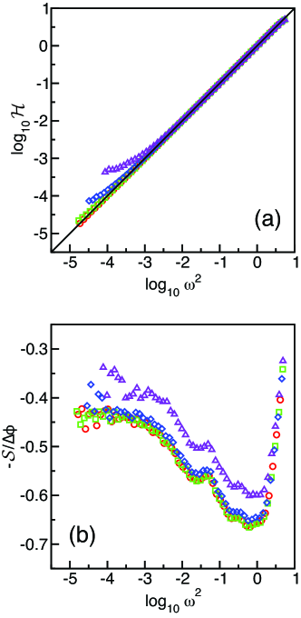
Figure 14: The two contributions to the dynamical matrix eigenvalues, (a) ${\cal H}$ and (b) $-{\cal S}/\Delta\phi$, plotted versus the eigenvalues of the dynamical matrix $\omega^{2}$ for bidisperse disk packings at $\Delta\phi=10^{-6}$ (circles), $10^{-5}$ (squares), $10^{-4}$ (diamonds), and $10^{-3}$ (triangles). In (a) the solid line corresponds to ${\cal H}=\omega^{2}$. Note that $-{\cal S}<0$ over the entire range of frequencies.

III.3 Quartic modes

We showed in Sec. III.1 that the dynamical matrix $M$ for packings of ellipsoidal particles contains a complete spectrum of $Nd_{f}-d$ nonzero eigenvalues $m_{i}$ for $\Delta\phi>0$ despite that fact that $z<z_{\rm iso}$. Further, we showed that the modes in the lowest frequency band scale as $\omega_{1}\sim(\Delta\phi)^{1/2}$ in the $\Delta\phi\rightarrow 0$ limit. What happens at jamming onset when $\Delta\phi=0$, i.e. are these low-frequency modes that become true zero-frequency modes at $\Delta\phi=0$ stabilized or destabilized by higher-order terms in the expansion of the potential energy in powers of the perturbation amplitude?

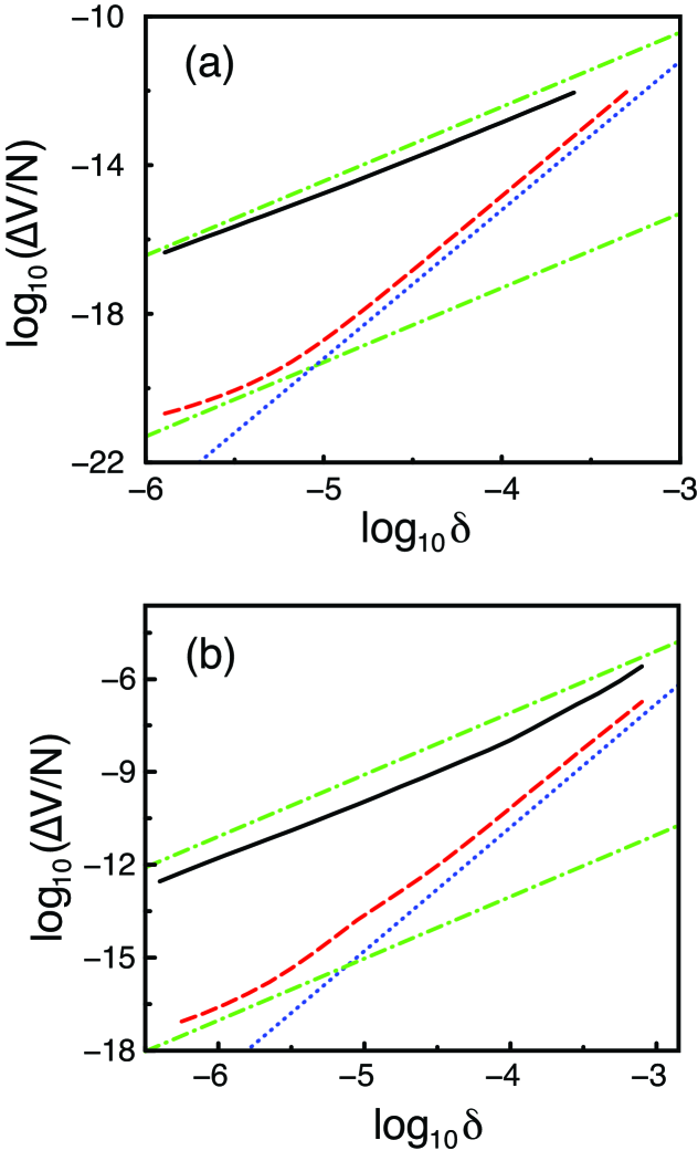
Figure 15: The change in the total potential energy $\Delta V$ (normalized by the particle number $N$) before and after applying the perturbation in Eq. 18 with amplitude $\delta$ along the eigenvector that corresponds to the lowest nontrivial eigenvalue of the dynamical matrix for packings of (a) disks (solid line) and ellipses with $\alpha=1.1$ (dashed line) and (b) spheres (solid line) and prolate ellipsoids with $\alpha=1.1$ (dashed line) at $\Delta\phi=10^{-7}$. The dot-dashed (dotted) lines have slope $2$ ($4$).

To investigate this question, we apply the following deformation to static packings of ellipsoidal particles:

$${\vec{u}}={\vec{u}}_{0}+\delta{\hat{m}}_{i},$$ (18)

where $\delta$ is the amplitude of the perturbation, ${\hat{m}}_{i}$ is an eigenvector of the dynamical matrix, and ${\vec{u}}_{0}$ is the point in configuration space corresponding to the original static packing, followed by conjugate gradient energy minimization. We then measure the change in the total potential energy before and after the perturbation, $\Delta V$.

We plot $\Delta V/N$ versus $\delta$ in Fig. 15 for perturbations along eigenvectors that correspond to the smallest nontrivial eigenvalue $m_{1}=\omega_{\rm min}^{2}$ of the dynamical matrix for static packings of (a) disks and ellipses and (b) spheres and prolate ellipsoids at $\Delta\phi=10^{-7}$. As expected, for disks and spheres, we find that $\Delta V/N\approx m\omega_{\rm min}^{2}\delta^{2}$ over a wide range of $\delta$ in response to perturbations along eigenvectors that correspond to the smallest nontrivial eigenvalue. In contrast, we find novel behavior for $\Delta V/N$ when we apply perturbations along the eigendirection that corresponds the lowest nonzero eigenvalue of the dynamical matrix for packings of ellipsoidal particles. In Fig. 16, we show that $\Delta V/N$ obeys

$$\frac{\Delta V}{N}=\frac{m}{2}\omega_{k}^{2}\delta^{2}+c_{k}\delta^{4},$$ (19)

where $\omega_{k}\propto\Delta\phi^{1/2}$ and the constants $c_{k}>0$, for perturbations along all modes $k$ in the lowest frequency band of $D(\omega)$ for packings of ellipsoidal particles when we do not include changes in the contact network following the perturbation and relaxation. (See Appendix A for measurements of $\Delta V/N$ when we include changes in the contact network.) Eigenmodes in the lowest frequency band are termed ‘quartic’ because at $\Delta\phi=0$ they are stabilized by quartic terms in the expansion of the total potential energy with respect to small displacements Mailman .

For $\delta\ll\delta_{k}^{*}$, the change in potential energy scales as $\Delta V/N\sim\omega_{k}^{2}\delta^{2}$, whereas $\Delta V/N\sim c_{k}\delta^{4}$ for $\delta\gg\delta_{k}^{*}$, where the characteristic perturbation amplitude $\delta_{k}^{*}=\omega_{k}\sqrt{m/2c_{k}}$. In the insets to Fig. 16 (a) and (b), we show that the characteristic perturbation amplitude averaged over modes in the lowest frequency band scale as $\delta^{*}\sim(\Delta\phi)^{1/2}/(\alpha-1)^{1/4}$ for static packings of ellipses in 2D and prolate ellipsoids in 3D, which indicates that the $c_{k}$ possess nontrivial dependence on aspect ratio $\alpha$.

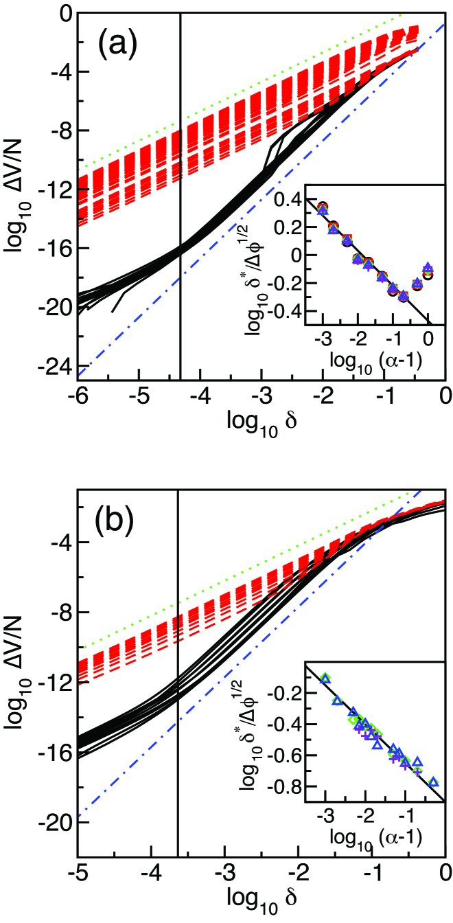
Figure 16: The change in the total potential energy $\Delta V/N$ for perturbations along the ‘quartic’ modes (solid) and all other modes (dashed) as a function of amplitude $\delta$ for (a) ellipses and (b) prolate ellipsoids with $\alpha=1.1$ for $\Delta\phi=10^{-7}$. The dotted (dot-dashed) lines have slope $2$ ($4$). The solid vertical lines indicate the characteristic amplitude $\delta^{*}$ at which $\Delta V/N$ crosses over from quadratic to quartic scaling averaged over the quartic modes. The insets show the scaling of $\delta^{*}/(\Delta\phi)^{1/2}$ with $\alpha-1$ for several values of compression: $\Delta\phi=10^{-8}$ (circles) and $10^{-7}$ (squares) for 2D systems and $10^{-6}$ (diamonds), $10^{-5}$ (triangles), and $10^{-4}$ (pluses) for both 2D and 3D systems. The solid lines in the insets have slope $-0.25$.

The quartic modes have additional interesting features. For example, quartic modes are dominated by the rotational rather than translational degrees of freedom. We identify the relative contributions of the translational and rotational degrees of freedom to the eigenvectors of the dynamical matrix in Figs. 17 and 18. The contribution of the translational degrees of freedom to eigenvector ${\hat{m}}_{i}$ is defined as

$$T_{i}=\sum_{j=1}^{Nd_{f}}\sum_{\lambda}(m_{\lambda i}^{j})^{2},$$ (20)

where the sum over $\lambda$ includes $x$ and $y$ in 2D and $x$, $y$, and $z$ in 3D and the eigenvectors are indexed in increasing order of the corresponding eigenvalues. Since the eigenvectors are normalized, the rotational contribution to each eigenvector is $R_{i}=1-T_{i}$.

For both ellipses in 2D and prolate ellipsoids in 3D, we find that at low aspect ratios ($\alpha<1.1$), the first $N$ ($2N$) modes in 2D (3D) are predominately rotational and the remaining $2N$ ($3N$) modes in 2D (3D) are predominately translational. In the inset to Figs. 17(b) and 18, we show that $T$ increases as $(\alpha-1)^{\zeta}$, where $\zeta\approx 1.5$ ($1.25$) for ellipses (prolate ellipsoids), for both the low and intermediate frequency modes. For $\alpha>1.2$, we find mode-mixing, especially at intermediate frequencies, where modes have finite contributions from both the rotational and translational degrees of freedom. For $\alpha\leq 1.2$, the modes become increasingly more translational with increasing frequency. For $\alpha>1.2$, the modes become more rotational in character at the highest frequencies. Our results show that the modes with significant rotational content at low $\alpha$ correspond to modes in the low and intermediate frequency bands of $D(\omega)$, while the modes with significant translational content at low $\alpha$ correspond to modes in the high frequency band of $D(\omega)$.

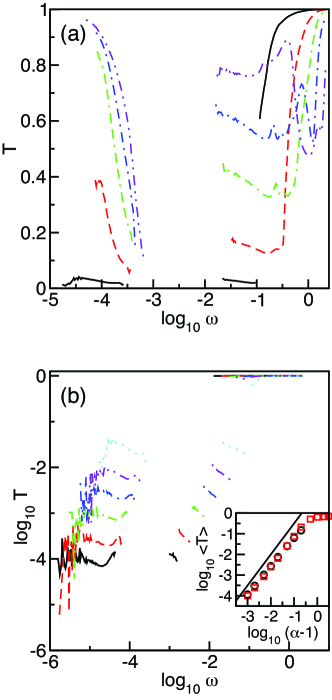
Figure 17: The contribution of the translational degrees of freedom $T$ to each eigenvector ${\hat{m}}$ of the dynamical matrix versus frequency $\omega$ in packings of ellipses in 2D at $\Delta\phi=10^{-7}$. (a) shows data for aspect ratios $\alpha=1.05$ (black solid), $1.2$ (red dashed), $1.5$ (green dash-dash-dot), $2.0$ (blue dash-dot), and $4.0$ (purple dot-dot-dash) and (b) shows data for aspect ratios $\alpha=1.001$ (black solid), $1.002$ (red dashed), $1.005$ (green dot-dot-dash), $1.01$ (blue dash-dot), $1.02$ (purple dot-dot-dash), and $1.05$ (cyan dotted). The inset to (b) shows $\langle T\rangle$ averaged over modes in the lowest (squares) and intermediate (circles) frequency regimes. The solid line has slope $1.5$.

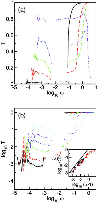
Figure 18: The contribution of the translational degrees of freedom $T$ to each eigenvector ${\hat{m}}$ of the dynamical matrix versus frequency $\omega$ in packings of prolate ellipsoids in 3D at $\Delta\phi=10^{-6}$. (a) shows data for aspect ratios $\alpha=1.01$ (black solid), $1.05$ (red dashed), $1.1$ (green dash-dash-dot), $1.2$ (blue dash-dot), and $1.5$ (purple dot-dot-dash) and (b) shows data for aspect ratios $\alpha=1.001$ (black solid), $1.002$ (red dashed), $1.005$ (green dash-dash-dot), $1.01$ (blue dash-dot), $1.02$ (purple dot-dot-dash), and $1.05$ (cyan dotted). The inset to (b) shows $\langle T\rangle$ averaged over modes in the lowest (squares) and intermediate (circles) frequency regimes. The solid line has slope $1.25$.

III.4 Protocol dependence

We performed several checks to test the robustness and accuracy of our calculations of the density of vibrational modes in the harmonic approximation $D(\omega)$ for static packings of ellipsoidal particles: 1) We compared $D(\omega)$ obtained from static packings of ellipsoidal particles using Perram and Wertheim’s exact expression (Eq. 2) for the contact distance between pairs of ellipsoidal particles and the Gay-Berne approximation described in Sec. II.1; 2) We calculated $D(\omega)$ for static packings as a function of the tolerance used to terminate energy minimization for both the MD and CG methods; and 3) We studied the system-size dependence of $D(\omega)$ in systems ranging from $N=30$ to $960$ particles.

In Fig. 19, we show that the density of vibrational modes $D(\omega)$ is nearly the same when we use the Perram and Wertheim exact expression and the Gay-Berne approximation to the contact distance for ellipse-shaped particles. $D(\omega)$ for static packings of ellipse-shaped particles is also not dependent on $V_{\rm tol}$, which controls the accuracy of the conjugate gradient energy minimization (Sec. II.2), for sufficiently small values. Our calculations in Fig. 19 (b) also show that $D(\omega)$ is not sensitive to the energy minimization procedure (i.e. MD vs. CG) for small values of the minimization tolerance $K_{\rm tol}$.

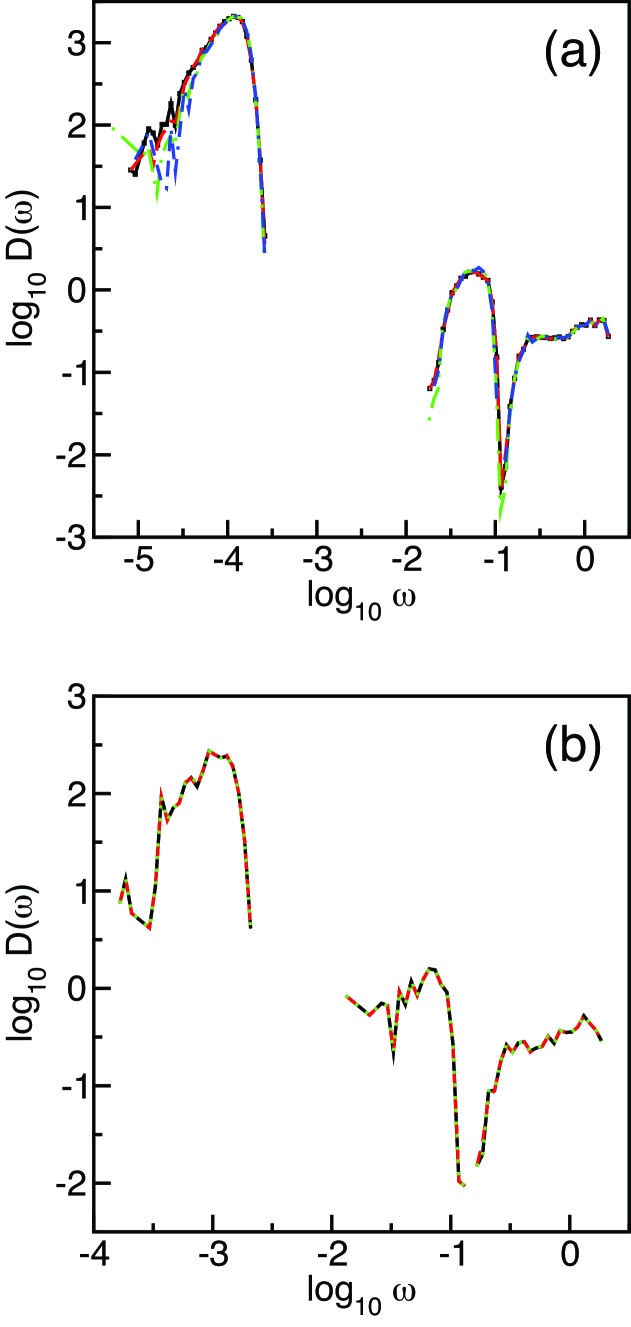
Figure 19: (a) Density of vibrational modes in the harmonic approximation $D(\omega)$ for $N=30$ ellipses with $\alpha=1.05$ at $\Delta\phi=10^{-7}$ using the Perram and Wertheim exact contact distance between pairs of ellipses with CG energy minimization tolerance $V_{\rm tol}=10^{-16}$ (green dot-dashed) and $V_{\rm tol}=10^{-8}$ (blue dash-dash-dotted) or the Gay-Berne approximation with $V_{\rm tol}=10^{-16}$ (black solid) and $V_{\rm tol}=10^{-8}$ (red dashed). (b) $D(\omega)$ for $N=12$ ellipses with $\alpha=1.05$ at $\Delta\phi=10^{-5}$ using the Perram and Wertheim exact contact distance with CG energy minimization tolerance $V_{\rm tol}=10^{-16}$ (solid black), and MD energy minimization tolerance $K_{\rm tol}=10^{-16}$ (red dashed) and $10^{-24}$ (green dotted).

In addition, key features of the density of vibrational modes are not strongly dependent on system size. For example, in Fig. 20, we show $D(\omega)$ for ellipses in 2D at aspect ratio $\alpha=1.05$ and compression $\Delta\phi=10^{-7}$ over a range of system sizes from $N=30$ to $960$. (For reference, $D(\omega)$ at fixed system size $N=240$ and $\Delta\phi=10^{-8}$ over a range of aspect ratios is shown in Fig. 7.) $D(\omega)$ in the low and intermediate frequency bands and plateau region overlap for all system sizes. The only feature of $D(\omega)$ that changes with system size is that successively lower frequency, long wavelength translational modes extend from the plateau region as system size increases. In the large system-size limit $N>(\phi-\phi_{J})^{-2}$, which we do not reach in these studies, the lowest frequency modes will scale as $D(\omega)\sim\omega^{d-1}$.

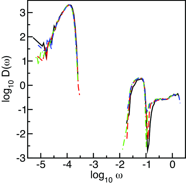
Figure 20: Density of vibrational modes in the harmonic approximation $D(\omega)$ for ellipses in 2D with aspect ratio $\alpha=1.05$, $\Delta\phi=10^{-7}$, and system size $N=30$ (black solid), $120$ (red dashed), $240$ (green dot-dashed), and $960$ (blue dash-dash-dotted).

IV Conclusions

We performed extensive numerical simulations of static packings of frictionless, purely repulsive ellipses in 2D and prolate ellipsoids in 3D as a function of aspect ratio $\alpha$ and compression from jamming onset $\Delta\phi$. We found several important results that highlight the significant differences between amorphous packings of spherical and ellipsoidal particles near jamming. First, as found previously, static packings of ellipsoidal particles generically satisfy $z<z_{\rm iso}$ Mailman ; zeravcic ; torquato_ellipse ; delaney ; i.e. they possess fewer contacts than the minimum required for mechanical stability as predicted by counting arguments that assume all contacts give rise to linearly independent constraints on particle positions. Second, we decomposed the dynamical matrix $M=H-S$ into the stiffness $H$ and stress $S$ matrices. We found that the stiffness matrix possesses $N(z_{\rm iso}-z)$ eigenmodes ${\hat{e}}_{0}$ with zero eigenvalues over a wide range of compressions $(\Delta\phi>0)$. Third, we found that the modes ${\hat{e}}_{0}$ are nearly eigenvectors of the dynamical matrix (and the stress matrix $-S$) with eigenvalues that scale as $c\Delta\phi$, with $c>0$, and thus finite compression stabilizes packings of ellipsoidal particles Mailman . At jamming onset, the harmonic response of packings of ellipsoidal particles vanishes, and the total potential energy scales as $\delta^{4}$ for perturbations by amplitude $\delta$ along these ‘quartic’ modes, ${\hat{e}}_{0}$. In addition, we have shown that these results are robust; for example, the density of vibrational modes $D(\omega)$ (in the harmonic approximation) is not sensitive to the error tolerance of the energy minimization procedure, the system size, and the accuracy of the determination of the interparticle contacts over the range of parameters employed in the simulations.

These results raise several fundamental questions for static granular packings: 1) Which classes of particle shapes give rise to quartic modes?; 2) Is there a more general isostatic counting argument that can predict the number of quartic modes at jamming onset (for a given packing-generation protocol)?; and 3) Are systems with quartic modes even more anharmonic schreck2011 than packings of spherical particles in the presence of thermal and other sources of fluctuations? We will address these important questions in our future studies.

Appendix A Scaling Behavior of the Total Potential Energy

The scaling behavior of $\Delta V/N$ (shown in Figs. 15 and 16) as a function of the amplitude $\delta$ of the perturbation along the eigenmodes of the dynamical matrix is valid only when the original contact network of the perturbed static packing does not change. As shown in Fig. 21, $\Delta V/N$ does not obey the power-law scaling described in Eq. 19 when new interparticle contacts form. Note that changes in the contact network are more likely for systems with $\alpha\sim 1$ as shown previously in Ref. schreck2011 . In a future publication, we will measure the critical perturbation amplitude $\delta^{k}_{c}$ below which new contacts do not form and existing contacts do not change for each mode $k$. This work is closely related to determining the nonlinear vibrational response of packings of ellipsoidal and other anisotropic particles.

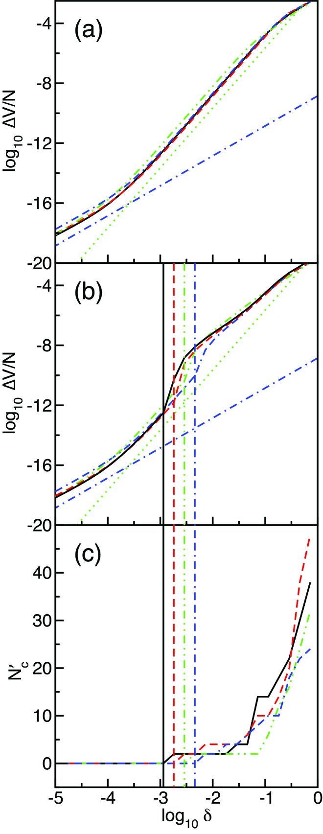
Figure 21: Change in the total potential energy $\Delta V/N$ when we (a) do not allow the system to gain contacts or (b) allow the system to gain contacts versus the amplitude of the perturbation $\delta$ along several ‘quartic’ modes (mode $17$: black solid, mode $23$: red dashed, mode $38$: green dot-dot-dashed, and mode $78$: blue dash-dash-dotted) from a static packing of $N=240$ ellipse-shaped particles at $\Delta\phi=10^{-8}$ and $\alpha=1.002$. The dotted (dot-dashed) line has slope $4$ ($2$). (c) The number of new contacts $N_{c}^{\prime}$ that differ from the original contact network as a function of $\delta$ for each mode in (a) and (b). The vertical lines indicate the $\delta$ at which the first new contact forms for each mode.

Appendix B Dynamical Matrix for Ellipse-shaped Particles

In this Appendix, we provide explicit expressions for the dynamical matrix elements (Eq. 11) for ellipse-shaped particles that interact via the purely repulsive linear spring potential (Eq. 1). The nine dynamical matrix elements for $i\neq j$ are

$$M_{x_{i}x_{j}} = \frac{F_{ij}}{r_{ij}^{3}}y_{ij}^{2}\bigg{(}1-\frac{\partial^{2}\ln\sigma_{ij}}{\partial\psi_{ij}^{2}}+\bigg{(}\frac{\partial\ln\sigma_{ij}}{\partial\psi_{ij}}\bigg{)}^{2}\bigg{)}+$$ (21)

$$\frac{G_{ij}}{r_{ij}^{2}}\bigg{(}x_{ij}+y_{ij}\frac{\partial\ln\sigma_{ij}}{\partial\psi_{ij}}\bigg{)}^{2}$$

$$M_{x_{i}y_{j}} = \frac{F_{ij}}{r_{ij}^{3}}x_{ij}y_{ij}\bigg{(}1-\frac{\partial^{2}\ln\sigma_{ij}}{\partial\psi_{ij}^{2}}+\bigg{(}\frac{\partial\ln\sigma_{ij}}{\partial\psi_{ij}}\bigg{)}^{2}\bigg{)}+$$

$$\frac{G_{ij}}{r_{ij}^{2}}\bigg{(}x_{ij}+y_{ij}\frac{\partial\ln\sigma_{ij}}{\partial\psi_{ij}}\bigg{)}\bigg{(}y_{ij}-x_{ij}\frac{\partial\ln\sigma_{ij}}{\partial\psi_{ij}}\bigg{)}$$

$$M_{x_{i}\theta_{j}} = l^{-1}\bigg{(}\frac{F_{ij}}{r_{ij}}\bigg{(}y_{ij}\frac{\partial^{2}\ln\sigma_{ij}}{\partial\psi_{ij}\partial\theta_{j}}-$$ (23)

$$\frac{\partial\ln\sigma_{ij}}{\partial\theta_{j}}\bigg{(}x_{ij}+y_{ij}\frac{\partial\ln\sigma_{ij}}{\partial\psi_{ij}}\bigg{)}\bigg{)}+$$

$$G_{ij}\frac{\partial\ln\sigma_{ij}}{\partial\theta_{j}}\bigg{(}x_{ij}+y_{ij}\frac{\partial\ln\sigma_{ij}}{\partial\psi_{ij}}\bigg{)}\bigg{)}\bigg{)}$$

$$M_{y_{i}x_{j}} = M_{x_{i}y_{j}}$$ (24)

$$M_{y_{i}y_{j}} = \frac{F_{ij}}{r_{ij}^{3}}x_{ij}^{2}\bigg{(}1-\frac{\partial^{2}\ln\sigma_{ij}}{\partial\psi_{ij}^{2}}+\bigg{(}\frac{\partial\ln\sigma_{ij}}{\partial\psi_{ij}}\bigg{)}^{2}\bigg{)}+$$ (25)

$$\frac{G_{ij}}{r_{ij}^{2}}\bigg{(}y_{ij}-x_{ij}\frac{\partial\ln\sigma_{ij}}{\partial\psi_{ij}}\bigg{)}^{2}$$

$$M_{y_{i}\theta_{j}} = l^{-1}\bigg{(}\frac{F_{ij}}{r_{ij}}\bigg{(}x_{ij}\frac{\partial^{2}\ln\sigma_{ij}}{\partial\psi_{ij}\partial\theta_{j}}-$$ (26)

$$\frac{\partial\ln\sigma_{ij}}{\partial\theta_{j}}\bigg{(}y_{ij}-x_{ij}\frac{\partial\ln\sigma_{ij}}{\partial\psi_{ij}}\bigg{)}\bigg{)}+$$

$$G_{ij}\frac{\partial\ln\sigma_{ij}}{\partial\theta_{j}}\bigg{(}y_{ij}-x_{ij}\frac{\partial\ln\sigma_{ij}}{\partial\psi_{ij}}\bigg{)}\bigg{)}\bigg{)}$$

$$M_{\theta_{i}x_{j}} = M_{x_{j}\theta_{i}}$$ (27)

$$\ M_{\theta_{i}y_{j}} = M_{y_{j}\theta_{i}}$$ (28)

$$\ M_{\theta_{i}\theta_{j}} = l^{-2}\bigg{(}F_{ij}r_{ij}\bigg{(}\frac{\partial\ln\sigma_{ij}}{\partial\theta_{i}}\frac{\partial\ln\sigma_{ij}}{\partial\theta_{j}}-\frac{\partial^{2}\ln\sigma_{ij}}{\partial\theta_{i}^{2}}\bigg{)}+$$ (29)

$$G_{ij}r_{ij}^{2}\bigg{(}\frac{\partial\ln\sigma_{ij}}{\partial\theta_{i}}\frac{\partial\ln\sigma_{ij}}{\partial\theta_{j}}\bigg{)}\bigg{)}$$

and the nine dynamical matrix elements for $i=j$ are

$$M_{x_{i}x_{i}} = -\sum_{j}M_{x_{j}x_{i}}$$ (30)

$$M_{x_{i}y_{i}} = -\sum_{j}M_{x_{j}y_{i}}$$ (31)

$$M_{x_{i}\theta_{i}} = -\sum_{j}M_{x_{j}\theta_{i}}$$ (32)

$$M_{y_{i}x_{i}} = M_{x_{i}y_{j}}$$ (33)

$$M_{y_{i}y_{i}} = -\sum_{j}M_{y_{j}y_{i}}$$ (34)

$$M_{y_{i}\theta_{i}} = -\sum_{j}M_{y_{j}\theta_{i}}$$ (35)

$$M_{\theta_{i}x_{i}} = M_{x_{i}\theta_{i}}$$ (36)

$$M_{\theta_{i}y_{i}} = M_{y_{i}\theta_{i}}$$ (37)

$$M_{\theta_{i}\theta_{i}} = l^{-2}\bigg{(}F_{ij}r_{ij}\bigg{(}\bigg{(}\frac{\partial\ln\sigma_{ij}}{\partial\theta_{i}}\bigg{)}^{2}-\frac{\partial^{2}\ln\sigma_{ij}}{\partial\theta_{i}^{2}}\bigg{)}+$$ (38)

$$G_{ij}r_{ij}^{2}\bigg{(}\frac{\partial\ln\sigma_{ij}}{\partial\theta_{i}}\bigg{)}^{2}\bigg{)},$$

where $\psi_{ij}$ is the polar angle defined in Fig. 5, $l=\sqrt{I/m}$, $F_{ij}$ is given in Eq. 6,

$$G_{ij} = \left|\frac{\partial^{2}V_{ij}(r_{ij}/\sigma_{ij})}{\partial r_{ij}^{2}}\right|=\sigma_{ij}^{-2},$$ (39)

$$\frac{\partial\ln\sigma_{ij}}{\partial\theta_{i}} = \frac{\chi}{2}\bigg{(}\frac{\sigma_{ij}}{\sigma_{ij}^{0}}\bigg{)}^{2}(\eta_{+}+\eta_{-})\bigg{(}\beta\cos^{2}(\theta_{i}-\psi_{ij})+$$ (40)

$$\frac{\chi}{2}(\eta_{+}-\eta_{-})\cos^{2}(\theta_{i}-\theta_{j})\bigg{)},$$

$$\frac{\partial^{2}\ln\sigma_{ij}}{\partial\psi_{ij}^{2}} = \frac{\chi}{2}\bigg{(}\frac{\sigma_{ij}}{\sigma_{ij}^{0}}\bigg{)}^{2}\bigg{(}\big{(}1+\chi\cos(\theta_{i}-\theta_{j})\big{)}\big{(}\nu_{+}^{2}-\eta_{+}^{2}\big{)}$$ (41)

$$+\big{(}1-\chi\cos(\theta_{i}-\theta_{j})\big{)}\big{(}\nu_{-}^{2}-\eta_{-}^{2}\big{)}\bigg{)}$$

$$+2\bigg{(}\frac{\partial\ln\sigma_{ij}}{\partial\psi_{ij}}\bigg{)}^{2}+\frac{\partial^{2}\ln\sigma_{ij}}{\partial\psi_{ij}^{2}}\bigg{|}_{\rm corr},$$

$$\frac{\partial^{2}\ln\sigma_{ij}}{\partial\psi_{ij}\partial\theta_{i}} = \frac{\chi}{2}\bigg{(}\frac{\sigma_{ij}}{\sigma_{ij}^{0}}\bigg{)}^{2}(\beta^{-1}\sin(\theta_{i}-\psi_{ij})(\eta_{+}-\eta_{-})-$$ (42)

$$\beta^{-1}\sin(\theta_{i}-\psi_{ij})$$

$$(\eta_{+}^{\prime}-\eta_{-}^{\prime})+$$

$$\chi\sin(\theta_{i}-\theta_{j})(\eta_{+}\eta_{+}^{\prime}-\eta_{-}\eta_{-}^{\prime}))$$

$$+2\bigg{(}\frac{\partial\ln\sigma_{ij}}{\partial\partial\theta_{i}}\bigg{)}\bigg{(}\frac{\partial\ln\sigma_{ij}}{\partial\psi_{ij}}\bigg{)}+\frac{\partial^{2}\ln\sigma_{ij}}{\partial\psi_{ij}\partial\theta_{i}}\bigg{|}_{\rm corr},$$

$$\frac{\partial^{2}\ln\sigma_{ij}}{\partial\theta_{i}^{2}} = \frac{\chi}{2}\bigg{(}\frac{\sigma_{ij}}{\sigma_{ij}^{0}}\bigg{)}^{2}\bigg{(}\chi\cos(\theta_{i}-\theta_{j})(\eta_{+}^{2}-\eta_{-}^{2})-$$ (43)

$$2\beta\cos(\theta_{i}-\psi_{ij})(\eta_{+}+\eta_{-})+\frac{4\beta^{2}\sin^{2}(\theta_{i}-\psi_{ij})}{1-\chi^{2}\cos^{2}(\theta_{i}-\theta_{j})}+$$

$$4\beta\chi\sin(\theta_{i}-\psi_{ij})\sin(\theta_{i}-\theta_{j})$$

$$\bigg{(}\frac{\eta_{+}}{1+\chi\cos(\theta_{j}-\theta_{i})}-\frac{\eta_{-}}{1-\chi\cos(\theta_{j}-\theta_{i})}\bigg{)}+$$

$$2\chi^{2}\sin(\theta_{i}-\theta_{j})^{2}$$

$$\bigg{(}\frac{\eta_{+}^{2}}{1+\chi\cos(\theta_{j}-\theta_{i})}+\frac{\eta_{-}^{2}}{1-\chi\cos(\theta_{j}-\theta_{i})}\bigg{)}+$$

$$2\bigg{(}\frac{\partial\ln\sigma_{ij}}{\partial\theta_{i}}\bigg{)}^{2}+\frac{\partial^{2}\ln\sigma_{ij}}{\partial\theta_{i}^{2}}\bigg{|}_{\rm corr},$$

$$\frac{\partial^{2}\ln\sigma_{ij}}{\partial\theta_{i}\partial\theta_{j}} = \frac{\chi}{2}\bigg{(}\frac{\sigma_{ij}}{\sigma_{ij}^{0}}\bigg{)}^{2}(\cos(\theta_{j}-\theta_{i})(\eta_{+}^{2}-\eta_{-}^{2})-$$ (44)

$$4\frac{\cos(\theta_{j}-\theta_{i})\sin(\theta_{i}-\psi_{ij})\sin(\theta_{j}-\psi_{ij})}{1-\chi^{2}\cos^{2}(\theta_{i}-\theta_{j})}+$$

$$2\beta\sin(\theta_{i}-\psi_{ij})\sin(\theta_{j}-\theta_{i})$$

$$\bigg{(}\frac{\eta_{+}}{1+\chi\cos(\theta_{i}-\theta_{j})}-\frac{\eta_{-}}{1-\chi\cos(\theta_{i}-\theta_{j})}\bigg{)}+$$

$$2\beta^{-1}\sin(\theta_{j}-\psi_{ij})\sin(\theta_{j}-\theta_{j})$$

$$\bigg{(}\frac{\eta_{+}}{1-\chi\cos(\theta_{i}-\theta_{j})}-\frac{\eta_{-}}{1+\chi\cos(\theta_{i}-\theta_{j})}\bigg{)}-$$

$$2\chi\sin^{2}(\theta_{j}-\theta_{i})$$

$$\bigg{(}\frac{\eta_{+}^{2}}{1-\chi\cos(\theta_{i}-\theta_{j})}+\frac{\eta_{-}^{2}}{1+\chi\cos(\theta_{i}-\theta_{j})}\bigg{)}-$$

$$2\frac{\partial\ln\sigma_{ij}}{\partial\theta_{i}}\frac{\partial\ln\sigma_{ij}}{\partial\theta_{j}}-\frac{\partial^{2}\ln\sigma_{ij}}{\partial\theta_{i}\partial\theta_{j}}\bigg{|}_{\rm corr},$$

$$\eta_{\pm} = \frac{\beta\cos(\theta_{i}-\psi_{ij})\pm\beta^{-1}\cos(\theta_{j}-\psi_{ij})}{1\pm\chi\cos(\theta_{i}-\theta_{j})},$$ (45)

$$\eta_{\pm}^{\prime} = \frac{\beta\sin(\theta_{i}-\psi_{ij})\pm\beta^{-1}\sin(\theta_{j}-\psi_{ij})}{1\pm\chi\cos(\theta_{i}-\theta_{j})},$$ (46)

and

$$\frac{\partial^{2}\ln\sigma_{ij}}{\partial\psi_{ij}^{2}}\bigg{|}_{\rm corr} = \frac{\partial^{2}\sigma_{ij}(\lambda)}{\partial\lambda^{2}}\bigg{(}\frac{\partial\lambda}{\partial\psi_{ij}}\bigg{)}^{2},$$ (47)

$$\frac{\partial^{2}\ln\sigma_{ij}}{\partial\psi_{ij}\partial\theta_{i}}\bigg{|}_{\rm corr} = \frac{\partial^{2}\sigma_{ij}(\lambda)}{\partial\lambda^{2}}\frac{\partial\lambda}{\partial\psi_{ij}}\frac{\partial\lambda}{\partial\theta_{i}},$$ (48)

$$\frac{\partial^{2}\ln\sigma_{ij}}{\partial\theta_{i}^{2}}\bigg{|}_{\rm corr} = \frac{\partial^{2}\sigma_{ij}(\lambda)}{\partial\lambda^{2}}\bigg{(}\frac{\partial\lambda}{\partial\theta_{i}}\bigg{)}^{2},$$ (49)

$$\frac{\partial^{2}\ln\sigma_{ij}}{\partial\theta_{i}\partial\theta_{j}}\bigg{|}_{\rm corr} = \frac{\partial^{2}\sigma_{ij}(\lambda)}{\partial\lambda^{2}}\frac{\partial\lambda}{\partial\theta_{i}}\frac{\partial\lambda}{\partial\theta_{j}}.$$ (50)

References

- (1) G. D. Scott, Nature 188 (1960) 908.
- (2) J. D. Bernal and J. Mason, Nature 188 (1960) 910.
- (3) G.-J. Gao, J. Blawzdziewicz, C. S. O’Hern, and M. D. Shattuck, Phys. Rev. E 80 (2009) 061304.
- (4) J. G. Berryman, Phys. Rev. A 27 (1983) 1053.
- (5) S. Torquato, T. M. Truskett, and P. G. Debenedetti, Phys. Rev. Lett. 84 (2000) 2064.
- (6) C. S. O’Hern, L. E. Silbert, A. J. Liu, and S. R. Nagel, Phys. Rev. E 70 043302 (2004).
- (7) G. Parisi and F. Zamponi, J. Chem. Phys. 123 (2005) 144501.
- (8) H. Jacquin, L. Berthier, and F. Zamponi, Phys. Rev. Lett. 106 (2011) 135702.
- (9) A. Donev, S. Torquato, F. H. Stillinger, Phys. Rev. E 71 (2005) 011105.
- (10) A. V. Tkachenko and T. A. Witten, Phys. Rev. E 60 (1999) 687.
- (11) For systems with ‘rattler’ particles that possess fewer than contacts, () for fixed (periodic) boundary conditions, where and is the number of rattler particles.
- (12) H. A. Makse, D. L. Johnson, and L. M. Schwartz, Phys. Rev. Lett. 84 (2000) 4160.
- (13) A. Donev, S. Torquato, F. H. Stillinger, and R. Connelly, J. Appl. Phys. 95 (2004) 989.
- (14) A. Donev, R. Connelly, F. H. Stillinger, and S. Torquato, Phys. Rev. E 75 (2007) 051304.
- (15) M. Mailman, C. F. Schreck, C. S. O’Hern, and B. Chakraborty, Phys. Rev. Lett. 102 (2009) 255501.
- (16) Z. Zeravcic, N. Xu, A. J. Liu, S. R. Nagel, and W. van Saarloos, Europhys. Lett. 87 (2009) 26001.
- (17) G. Delaney, D. Weaire, S. Hutzler, and S. Murphy, Phil. Mag. Lett. 85 (2005) 89.
- (18) W. N. Man, A. Donev, F. H. Stillinger, M. T. Sullivan, W. B. Russel, D. Heeger, S. Inati, S. Torquato, and P. M. Chaikin, Phys. Rev. Lett. 94 (2005) 198001.
- (19) A. Donev, I. Cisse, D. Sachs, E. A. Variano, F. H. Stillinger, R. Connelly, S. Torquato, and P. M. Chaikin, Science 303 (2004) 990.
- (20) K. C. Smith, M. Alam, and T. Fisher, “Isostaticity of constraints in jammed systems of soft frictionless platonic solids” (preprint) 2011.
- (21) A. Tanguy, J. P. Wittmer, F. Leonforte, and J.-L. Barrat, Phys. Rev. B 66 (2002) 174205.
- (22) P. J. Yunker, K. Chen, Z. Zhang, W. G. Ellenbroek, A. J. Liu, and A. G. Yodh, Physical Review E 83 (2011) 011403.
- (23) C. F. Schreck and C. S. O’Hern, “Computational methods to study jammed systems”, in Experimental and Computational Techniques in Soft Condensed Matter Physics, ed. by J. S. Olafsen, (Cambridge University Press, New York, 2010).
- (24) C. F. Schreck, N. Xu, and C. S. O’Hern, Soft Matter 6 (2010) 2960.
- (25) B. J. Berne and P. Pechukas, J. Chem. Phys. 56 (1972) 4213.
- (26) J. G. Gay and B. J. Berne, J. Comp. Phys. 74 (1981) 3316.
- (27) D. J. Cleaver, C. M. Care, M. P. Allen, M. P Neal, Phys. Rev. E 54 (1996) 559.
- (28) J. W. Perram and M. S. Wertheim, J. Comp. Phys. 58 (1985) 409.
- (29) J. W. Perram, J. Rasmussen, E. Prstgaard, and J. L. Lebowitz, Phys. Rev. E. 54 (1996) 6565.
- (30) N. Xu, J. Blawzdziewicz, and C. S. O’Hern, Phys. Rev. E 71 (2005) 061306.
- (31) G.-J. Gao, J. Blawzdziewicz, and C. S. O’Hern, Phys. Rev. E 74 (2006) 061304.
- (32) The CG gradient energy minimization technique we implement relies on numerous evaluations of the total potential energy to identify local minima. However, when we integrate Newton’s equations of motion with damping forces proportional to particle velocities (Eqs. 3 and 4), energy minimization and the minimization stopping criteria are based on the evaluation of forces and torques, which allows increased accuracy compared to the CG technique.
- (33) M. P. Allen and D. J. Tildesley, Computer Simulation of Liquids (Oxford University Press, New York, 1987).
- (34) C. F. Schreck, T. Bertrand, C. S. O’Hern, and M. D. Shattuck, Phys. Rev. Lett. 107 (2011) 078301.
- (35) Since we employ overdamped energy minimization dynamics, rattler particles can contact non-rattler particles with interparticle separation .
- (36) L. E. Silbert, A. J. Liu, and S. R. Nagel, Phys. Rev. Lett. 95 (2005) 098301.
- (37) M. Wyart, L. E. Silbert, S. R. Nagel, and T. A. Witten, Phys. Rev. E 72 (2005) 051306.