Tadpole cancellation in top-quark condensation

Abstract

We show that quadratic divergences in top-quark condensation are cancelled when the tadpoles cancel. This latter cancellation is naturally implemented as the cancellation among the top-quark, Goldstone and Higgs contributions. We also calculate the bosonic correction terms to Gribov’s mass formula for the Higgs boson. These reduce the prediction for $M_{H}$ from $167$ GeV to $132$ GeV. The tadpole cancellation condition by itself is an independent condition on the mass of the Higgs boson which, in Gribov’s U(1)_Y scenario, yields $M_{H}\approx 117$ GeV with large theoretical uncertainty. More generally, we are able to obtain all three masses, $M_{W}$, $m_{t}$ and $M_{H}$, in $100$ MeV to $10$ TeV energy range as a function of the cut-off scale and the gauge couplings only.

I Introduction

As is well known, the Standard Model, with an elementary Higgs doublet field, suffers from the problem of quadratic divergences when radiative corrections, due to the loops of fermions, the top quark in particular, to the mass of the Higgs boson is calculated. This problem is often referred to as the hierarchy problem, as we require an artificial fine tuning between the induced radiative mass, which is of the order of the cut-off scale, e.g., $\mathcal{O}(M_{\mathrm{Pl}})$, and the counterterm to produce a mass of the order of the electroweak scale.

This tempts us to speculate that the Higgs boson may in fact be composite. The simplest implementation of this idea is top-quark condensation nambu ; bardeen ; topcondensation . It turns out, however, that this compositeness by itself is not sufficient to remove the problem of quadratic divergences, and fine tuning is still required in the simpler approaches to top-quark condensation.

The problem of divergences can only be artificial, because the same loop corrections, applied to the mass of the Goldstone bosons, produce a similar quadratic divergence, whereas the Goldstone theorem guarantees that spontaneous symmetry breaking results in massless Goldstone bosons. This suggests that these quadratic divergences are an artifact, and will vanish if the condition of current conservation is implemented properly.

For example, the approach of Chesterman, King and Ross bethe_salpeter uses the vanishing of the mass of the Goldstone boson as a consistency check, and is able to obtain sensible values for the mass of the Higgs boson.

A more direct investigation into this point regarding current conservation was made by Gribov in ref. gribovewsb , and his results are in quantitative agreement with ref. bethe_salpeter . In that paper, he implemented the symmetry condition, somewhat by force, by requiring that the Goldstone-boson self-energy vanishes in the soft limit. The mass of the Higgs boson is then obtained by subtracting off the Goldstone-boson self-energy, leading to the following Pagels–Stokar-type equation for the mass of the Higgs boson:

$$M_{H}^{2}=\frac{N_{C}}{2v^{2}\pi^{2}}\int_{m_{t}^{2}}^{\lambda^{2}}\frac{dq^{2}}{q^{2}}m_{t}^{4}(q^{2}).$$ (1)

This gives the mass $M_{H}=167$ GeV for the Higgs boson using the top-quark mass $m_{t}=174$ GeV and $\alpha_{S}=0.11$ as input. Gribov’s cut-off $\lambda$ is given by the U(1)_Y Landau pole, $\sim 10^{42}$ GeV, but the results are relatively insensitive to the value of the cut-off scale. This value of $M_{H}$ is not far from the recent LHC results cernpressrelease ; atlashiggs ; cmshiggs which suggest $M_{H}\approx 125$ GeV. It is worth noting here that eqn. (1) is general and is independent of the physics that causes the cut-off.

Our questions are the following. First, what may be the justification for this procedure, in particular the mechanism for the cancellation of the divergences? Second, whether there may be correction terms due to the loops of Goldstone and Higgs bosons in eqn. (1).

Concerning the first question, we shall show in this paper that the quadratic divergences are proportional to the tadpole and therefore vanish when the vacuum is stable. Although this statement must be independent of the basis, it is most easily verified by defining the Goldstone bosons as the divergence of the weak current so that derivative couplings do not arise.

Our analysis is quite general in the sense that no new interactions are introduced up to the UV cut-off scale. This procedure has the well-known phenomenological disadvantage that the mass $M_{W}$ of the $W$ boson is predicted to be too low for fixed $m_{t}$ or, equivalently, $m_{t}$ is predicted to be too large for fixed $M_{W}$. This is partially alleviated by taking large $\lambda$ such as, as in Gribov’s scenario, the U(1)_Y Landau pole. Even this is not sufficient and, as remarked in ref. gribovewsb , more UV contribution is required, which may be, one would naturally guess, due to strong dynamics at near and above the cut-off.

The methods of our analysis are analogous to those in ref. odagirimagnetism that are worked out in the context of anti-ferromagnetism. The second of the questions above is also addressed within this framework, and we find that the correction to eqn. (1) is large and negative.

As an explanation of our framework, we implement current conservation by requiring the vanishing of the Ward–Takahashi identities. This fixes the bosonic three-point and four-point couplings. In other words, the shape of the Higgs potential is fixed by current conservation, and this turns out to be of the same form as that of the Standard Model. We then implement the vacuum-stability condition, namely that the Higgs $\to X$ one-point function, or the tadpole, vanishes.

Note that the cancellation of the tadpole, which is imposed as the cancellation among the top-quark, Goldstone-boson and Higgs-boson loops, is by itself an independent condition on the symmetry-breaking parameters. This yields

$$M_{H}^{2}\approx 8m_{t}^{2}(\lambda^{2}),$$ (2)

which implies $M_{H}\approx 117$ GeV in the U(1)_Y scenario, if we only include the QCD part of the running. This is very close to the LHC value, but this remarkable success should not be taken too seriously, because this condition will be affected by the renormalization, due to the U(1)_Y interaction, of the top-quark mass at near the Landau pole.

It should be noted that this extra condition on the Higgs mass, in principle, completely fixes the symmetry-breaking parameters. That is, all three masses, $M_{W}$, $m_{t}$ and $M_{H}$, are fixed for given values of the cut-off scale and gauge couplings. This provides a natural solution to the hierarchy problem and, indeed, we obtain a large hierarchy that is comparable with the actual hierarchy between the UV and EWSB scales.

The form of the UV theory does not affect our analysis at the present level of approximation, so long as the symmetry is spontaneously broken by a UV condensate which exists only at high energies. This requires a supercritically strong UV interaction, and a natural candidate is Gribov’s U(1)_Y scenario. We discuss the physics of this scenario.

II Current conservation conditions

Tadpole cancellation in bosonic self-energy was, in part, discussed by Gribov himself in the context of chiral symmetry breaking in ref. gribovlongshort . However, he imposes tadpole cancellation there by introducing a boson–boson–quark–quark term (e.g., eqn. (132) of ref. gribovlongshort ) to cancel the anomalous term in the Ward–Takahashi identity associated with Compton scattering. One problem in doing so is that this will lead to the necessity of introducing an infinite number of $N$-boson–quark–quark couplings.

In ref. odagirimagnetism , and in the context of anti-ferromagnetism, we proposed a more economical mechanism which also seems to us to be more natural. Here, only the three-point and four-point couplings among the Goldstone and Higgs bosons are needed, and these couplings are fixed by symmetry conditions such as the Ward–Takahashi identities.

We shall demonstrate that the couplings are consistent with the Standard-Model-like quartic Higgs potential. In the low-energy effective theory, the phenomenology is identical to that of the Standard Model, at least insofar as the couplings to the bosons and the top quark are concerned. As for the other fermionic Yukawa couplings, it is natural to assume that they are as given by the Standard Model though, strictly speaking, other possibilities cannot be ruled out.

Let us start with the fermionic vertex function for the left-handed SU(2) current. As discussed in ref. gribovewsb , Ward–Takahashi identity is satisfied by the following modified vertex:

(3)

Here, the small blob stands for the unmodified vertex $\frac{1}{2}\gamma_{\mu}^{L}\sigma^{a}$ and the two-point function ($f_{ab}p_{\mu}$ in Gribov’s notation) which follows from that, and the asterisk stands for the vertex that is modified by the inclusion of the Goldstone-boson contribution. The dashed line stands for one of the three Goldstone bosons $G^{0}$, $G^{\pm}$.

The Ward–Takahashi identity, applied to the modified vertex, fixes the $G$ coupling to fermions to be, for example,

$$g_{G^{0}}=i\gamma_{5}\sigma^{3}\frac{m}{2f},$$ (4)

where $f$, the Goldstone-boson form factor, is defined by the two-point function of eqn. (3). $f=v/2$, where $v$ is the usual ‘vacuum-expectation value of the Higgs field’. Note that the Feynman rules are, as usual, given by $-ig$. This will apply to all couplings that appear in the following.

The same exercise may be repeated for the bosonic vertex:

(5)

The unmodified vertex is necessarily proportional to $p_{G}+p_{H}$ (momenta flows left to right, or more generally $G$ to $H$) in order to satisfy the Ward–Takahashi identity, and the normalization is fixed by the Ward–Takahashi identity applied to the amplitude shown in fig. 1.

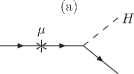
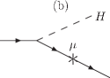
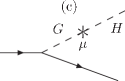
Figure 1: The three diagrams whose sum must satisfy the Ward–Takahashi identity.

This fixes the $GGH$ coupling to be:

$$g_{GGH}=\frac{M_{H}^{2}}{2f},$$ (6)

when the Yukawa coupling of the Higgs boson to fermions is given by

$$g_{H}=\frac{m}{2f}.$$ (7)

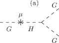
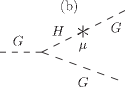
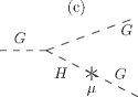
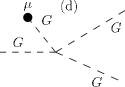
Figure 2: Four diagrams whose sum must satisfy the Ward–Takahashi identity. Not all diagrams are present for all combinations of $G$

Next, we consider the Ward–Takahashi identity in the set of amplitudes that are described by fig. 2. This allows us to work out the Goldstone-boson quartic couplings:

$$\left\{\begin{array}[]{l}g_{G^{+}G^{-}G^{0}G^{0}}=M_{H}^{2}/4f^{2},\\ g_{G^{+}G^{+}G^{-}G^{-}}=2M_{H}^{2}/4f^{2},\\ g_{G^{0}G^{0}G^{0}G^{0}}=3M_{H}^{2}/4f^{2}.\end{array}\right.$$ (8)

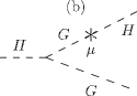
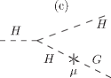
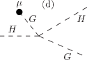
Figure 3: Four diagrams whose sum must satisfy the Ward–Takahashi identity.

We then turn to the set of amplitudes that are described by fig. 3, and obtain

$$g_{GGHH}=\frac{1}{f}\left(-g_{GGH}+\frac{g_{HHH}}{2}\right).$$ (9)

Note that the Higgs-boson self-coupling is not fixed by current conservation conditions but either by loops or by the symmetry between Goldstone and Higgs bosons. As noted in ref. gribovewsb , these turn out to be the same as the couplings of the Standard Model:

$$g_{HHH}=\frac{3M_{H}^{2}}{2f},\qquad g_{HHHH}=\frac{3M_{H}^{2}}{4f^{2}}.$$ (10)

This implies

$$g_{GGHH}=\frac{M_{H}^{2}}{4f^{2}}.$$ (11)

We notice that the effective Lagrangian for the multi-boson interaction terms can be written as

$$-\mathcal{L}_{\mathrm{eff}}=\frac{M_{H}^{2}}{8v^{2}}\left[2G^{+}G^{-}+(G^{0})^{2}+(v+H)^{2}-v^{2}\right]^{2}.$$ (12)

In terms of the Standard-Model Higgs-doublet field $\Phi$, this expression is proportional to $(\Phi^{\dagger}\Phi-v^{2})^{2}$. That is, the mass-generation mechanism of the effective theory is equivalent to that of the Standard Model.

III Tadpole cancellation

We now consider the tadpole cancellation condition:

(13)

Let us neglect the contribution of all fermions other than the top quark. This yields

$$\int_{m_{t}^{2}}^{\lambda^{2}}dq^{2}\left[N_{C}\frac{4m_{t}^{2}(q^{2})}{2f}-\frac{3}{2}\frac{M_{H}^{2}(0)+M_{H}^{2}(q^{2})}{2f}\right]=0,$$ (14)

where the simplification $q^{2}\gg m_{t}^{2},M_{H}^{2}$ has been made. The shorthand notation $m_{t}=m_{t}(m_{t}^{2})$ is used. Note that in the Goldstone loop, $M_{H}$ is not corrected by renormalization effects. This is in contrast to the Higgs-boson loop, which is suppressed because of the running Higgs mass. We have neglected the renormalization effects to $f^{2}$, which are relatively small, due to the Goldstone and Higgs boson propagators.

Since eqn. (14) is dominated by the large energy region, we then obtain

$$M_{H}^{2}(0)\approx 8m_{t}^{2}(\lambda^{2}),$$ (15)

as discussed in the introduction. Strictly speaking, the scale on the right-hand side should be slightly below $\lambda$. The running of the top quark mass is as given by eqn. (10) of ref. gribovewsb :

$$m_{t}(q^{2})=m_{t}\left(\alpha_{s}(q^{2})/\alpha_{s}(m_{t}^{2})\right)^{4/7},$$ (16)

where only the QCD part of the evolution is included, and

$$\alpha_{s}^{-1}(q^{2})=\alpha_{s}^{-1}(m_{t}^{2})+\frac{7}{4\pi}\ln\frac{q^{2}}{m_{t}^{2}}.$$ (17)

Figure 4: $M_{H}(0)$ as a function of the cut-off scale $\lambda$, using eqn. (15), for $m_{t}(m_{t})=174$ GeV. Only the QCD part of the evolution is included.

The result of eqn. (15) is shown in fig. 4. The U(1)_Y scenario yields $M_{H}=117$ GeV, when $\lambda$ ($\sim 10^{42}$ GeV) is given by eqns. (45) and (46) of ref. gribovewsb :

$$(\alpha^{\prime}(\lambda^{2}))^{-1}=(\alpha^{\prime}(m_{t}^{2}))^{-1}-\frac{5}{3\pi}\ln\frac{\lambda^{2}}{m_{t}^{2}}\approx 0.$$ (18)

As mentioned in the introduction, this spectacular agreement with the LHC results cernpressrelease ; atlashiggs ; cmshiggs should be treated with caution and suspicion. The full running $m_{t}$, which includes both QCD and U(1)_Y running, formally vanishes at the Landau pole. The reason for our omitting the latter running is that the effect is much less than the QCD running, except at very near the Landau pole. Furthermore, at near the Landau pole, the perturbative result for the running mass cannot be trusted.

Having said that, we may, as a means of error estimation, include the U(1)_Y running effect in eqn. (14) which is then evaluated literally. This yields $88$ GeV. Thus there is roughly 25 % error in our prediction of $M_{H}=117$ GeV.

Even so, this result provides some support to Gribov’s U(1)_Y scenario since, as can be seen from fig. 4, low $M_{H}$ requires large $\lambda$.

IV Bosonic self-energies

The three types of Feynman diagram for the self-energy of Goldstone and Higgs bosons are shown in fig. 5. We have not shown the tadpole diagrams of the form discussed in the previous section, as these are zero if the tadpole cancellation condition is imposed. The contributions of figs. 5a and c are quadratically divergent, and we shall show that they mutually cancel. The contribution of fig. 5b provides a correction to eqn. (1).

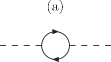
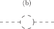
Figure 5: The diagrams for the self-energy of the Goldstone and Higgs bosons. Diagram b involves the $g_{GGH}$ and $g_{HHH}$ couplings, and diagram c involves $g_{GGHH}$, $g_{GGGG}$ and $g_{HHHH}$ couplings.

Let us consider the Goldstone-boson self-energy. At zero external momentum, the contributions of the three diagrams are given by:

$$\Sigma^{G}_{a} = \int\frac{d^{4}k}{(2\pi)^{4}i}\frac{m_{t}^{2}N_{C}}{4f^{2}}\mathrm{Tr}\left[\frac{1}{k^{2}-m_{t}^{2}}\right],$$ (19)

$$\Sigma^{G}_{b} = -\int\frac{d^{4}k}{(2\pi)^{4}i}\frac{M_{H}^{4}}{4f^{2}}\frac{1}{k^{2}(k^{2}-M_{H}^{2})},$$ (20)

$$\Sigma^{G}_{c} = -\int\frac{d^{4}k}{(2\pi)^{4}i}\frac{M_{H}^{2}}{4f^{2}}\left[\frac{5}{2k^{2}}+\frac{1}{2(k^{2}-M_{H}^{2})}\right].$$ (21)

We see that adding together these three equations yields zero so long as the tadpoles cancel. For a more formal, all-order treatment of such cancellations in the Goldstone-boson mass, we may, for instance, consider the non-vanishing part of $p^{\mu}\Delta\Pi_{\mu\nu}$ in eqn. (29) of ref. gribovewsb and show that this is equivalent to tadpole contributions. As a generalization, we note that the divergences cancel in any case in Goldstone-boson self-energy, regardless of the vanishing of the tadpoles, if the tadpole diagrams are added explicitly to fig. 5.

Because the Goldstone-boson self-energy must be equal to $-p^{2}$, calculating $\Sigma^{G}$ at finite and small external momentum allows us to work out $f$, and this reproduces eqn. (14) of ref. gribovewsb :

$$f^{2}=\frac{3}{2g_{s}^{2}}m_{t}^{2}\left[1-\left(\frac{\alpha_{s}(\lambda^{2})}{\alpha_{s}(m_{t}^{2})}\right)^{1/7}\right].$$ (22)

The bosonic contributions do not give logarithmic corrections to this equation. This equation predicts $m_{t}$ as a function of $M_{W}$, or vice versa and, as a generic problem in top-quark condensation approaches, it is well known that the predicted $m_{t}$ is too high. For example, Gribov gribovewsb predicts $m_{t}=215$ GeV for $\alpha_{s}(m_{t}^{2})=0.11$. In ref. gribovewsb , this discrepancy is attributed to UV contributions near the Landau pole due to the strong dynamics. This is one possibility, but another source of the discrepancy may be new contributions (e.g., gravitational) at high scales, since eqn. (22) is relatively sensitive to the mass evolution at high scales, unlike eqn. (1) which is affected by $m_{t}$ quartically and is therefore less sensitive to the UV region.

Let us now turn to the Higgs-boson self-energy. These are also given by the three diagrams shown in fig. 5. The amplitudes at zero external momentum are now given by

$$\Sigma^{H}_{a} = \int\frac{d^{4}k}{(2\pi)^{4}i}\frac{m_{t}^{2}N_{C}}{4f^{2}}\mathrm{Tr}\left[\frac{k^{2}+m_{t}^{2}}{(k^{2}-m_{t}^{2})^{2}}\right],$$ (23)

$$\Sigma^{H}_{b} = -\int\frac{d^{4}k}{(2\pi)^{4}i}\frac{M_{H}^{4}}{4f^{2}}\left[\frac{3}{2k^{4}}+\frac{9}{2(k^{2}-M_{H}^{2})^{2}}\right],$$ (24)

$$\Sigma^{H}_{c} = -\int\frac{d^{4}k}{(2\pi)^{4}i}\frac{M_{H}^{2}}{4f^{2}}\left[\frac{3}{2k^{2}}+\frac{3}{2(k^{2}-M_{H}^{2})}\right].$$ (25)

The sum of the quadratic divergences of $\Sigma^{H}_{a}$ and $\Sigma^{H}_{c}$ is proportional to the tadpole and therefore vanishes. We then obtain

$$M_{H}^{2}=\frac{6}{16\pi^{2}f^{2}}\int_{m_{t}^{2}}^{\lambda^{2}}\frac{dq^{2}}{q^{2}}\left[m_{t}^{4}(q^{2})-\frac{M_{H}^{4}(0)+3M_{H}^{4}(q^{2})}{16}\right].$$ (26)

The second term of eqn. (26) gives a correction to eqn. (1).

In order to solve this integral, we need the running $M_{H}^{2}$. This is obtained by writing the left-hand side of eqn. (26) as $M_{H}^{2}(Q^{2})$, changing the lower limit of integration to $Q^{2}$, and replacing $M_{H}(0)$ by $M_{H}(Q^{2})$. The low-energy Higgs mass, i.e. $M_{H}(0)$, is then obtained by solving the resulting integral equation numerically.

Figure 6: $M_{H}$ against the cut-off scale, with the bosonic correction (continuous line) and without (dotted line). Only the QCD part of the evolution is included.

The result of this calculation is shown in fig. 6, using $m_{t}=174$ GeV and $\alpha_{S}=0.11$. We see that in the U(1)_Y scenario, $M_{H}$ is reduced from 167 GeV to 132 GeV. $M_{H}$ also becomes more independent of $\lambda$, and we find that the maximum value $M_{H}\approx 141$ GeV is obtained for $\lambda\approx 10^{15}$ GeV.

Above $\lambda\approx 10^{10}$ GeV, the uncertainty, which may be estimated by varying $m_{t}$ and $\alpha_{S}$, becomes nearly constant. For example, by varying $m_{t}$ by $\pm 5$ GeV, we obtain $\pm 5$ GeV variation in $M_{H}$, and by varying $\alpha_{S}$ by $\pm 0.01$, we again obtain $\pm 5$ GeV variation in $M_{H}$. The combined error is thus $\pm 7$ GeV. Other sources of uncertainty are: the higher-order corrections which are expected to be small when the running couplings are small; the UV correction near the Landau pole; and other UV interactions which may be present.

Note that the Higgs mass prediction of fig. 4 is independent of the prediction of fig. 6. The former was obtained by the condition that the tadpole vanishes, and the latter was obtained by evaluating the self-energy integrals. If both predictions are literally true, it follows that the point at which the two predictions match, which comes out to be about $10^{32}$ GeV, is the true scale of the UV cut-off.

Another way of saying the same thing is that given a value of the UV cut-off, and the running coupling constants, we can work out all three of $M_{W}$, $m_{t}$ and $M_{H}$ as opposed to the previous studies in which $M_{H}$ is predicted for given $m_{t}$ and the cut-off, and so on. This follows because we now have three equations, namely eqns.  (14), (22) and (26), as opposed to two. The combined set of equations may be solved by solving the following integral equation:

$$\mu(r)=\int_{r}^{R}\frac{(R/r^{\prime})^{16/7}-4(\mu^{2}(r)+3\mu^{2}(r^{\prime}))}{14R(R^{1/7}-1)}dr^{\prime},$$ (27)

numerically, with the condition $\mu(R)=0$. We then search for a value of $R$ that satisfies $\mu(1)\equiv M_{H}^{2}/8m_{t}^{2}(\lambda^{2})=1$. By doing so, we obtain

$$R=\alpha_{s}(m_{t}^{2})/\alpha_{s}(\lambda^{2})=7.31.$$ (28)

This ratio corresponds to a significantly large hierarchy. We plot the resulting $m_{t}$ and $v$ as a function of the cut-off scale $\lambda$, in fig. 7. $M_{H}$ is indistinguishable from $m_{t}$ on the logarithmic scale.

Figure 7: $m_{t}$ and $v$ as a function of the cut-off scale $\lambda$, using eqn. (27) and eqn. (22). Only the QCD part of the evolution is included.

Taking $\lambda$ to be the U(1)_Y Landau scale yields

$$m_{t}=4.29\times 10^{4}\ \mathrm{GeV},$$ (29)

which is only two orders of magnitude away from the top-quark mass scale. In order to cover the two remaining orders of magnitude, we will need to resolve the $m_{t}/M_{W}$ discrepancy discussed below eqn. (22). We should mention here that the variations of $m_{t}$ and $\alpha_{S}$ cannot explain the two-orders-of-magnitude difference.

One should beware of hasty conclusions, from fig. 7, that the cut-off scale is at $\sim 10^{24}$ GeV. The numbers that are shown are sensitive to possible corrections, e.g., the choice of energy scale, in eqn. (14), and the need to produce a value of $v/m_{t}$ that is as large as the observed value favours large $\lambda$.

V Discussions

Our result shows that the electroweak scale is not necessarily fixed by the parameters at the UV scale. Rather, it is fixed by dimensional transmutation, and this in turn is governed by the condition of vacuum stability and the radiative effects.

What conditions are necessary, then, in order that symmetry breaking occurs in the first place?

In our opinion, it is sufficient that the symmetry is broken by a chiral condensate which appears at a high scale. This requires that a coupling constant becomes large. Gribov has shown gribovquarkconfinement that supercriticality and chiral symmetry breaking occurs when the relevant coupling constant satisfies

$$\alpha/\pi\gtrsim 0.137.$$ (30)

Gribov’s U(1)_Y scenario is a natural candidate, but one will then need to show that the gravitational coupling will not satisfy this condition. A possibility would be that gravitation is described by a weak-coupling theory above the Planck scale, becomes strongly coupled near the Planck scale, and reduces to Einstein gravity at low scales. For example, it may be that scale generation at the U(1)_Y pole is itself the source of scale generation in gravity.

It is interesting to ask, what might be the behaviour of the U(1)_Y coupling at high scales? This question was addressed partially in ref. odagirigribov . We argued that when the U(1)_EM coupling grows large, it will decouple as $\alpha\propto q^{2}$. The effective coupling experienced by the electrons is then given by

$$\left(1-\frac{d\ln\alpha}{d\ln q^{2}}\right)\alpha\longrightarrow\frac{1}{\left|b_{0}\right|},$$ (31)

where $b_{0}$ is the first coefficient of the beta function. If we can use the U(1)_Y beta function here, then the effective coupling will tend to $3\pi/5$, which is large compared with $0.137\pi$. Thus chiral symmetry breaking will almost certainly occur by U(1)_Y.

The condensate which appears at high scales must have decayed to fermions and Goldstone bosons at low scales, from phenomenological reasons. First, the observed masses of particles are light. Second, a condensate will lead to a cosmological constant which is much heavier than is observed.

If EWSB is due to the formation of the supercritical condensate at high scales, one must ask the question of whether the supercritical states might affect the running of the parameters. Our answer is that the Goldstone and the Higgs states are supercritical states, but the other states cannot affect the running, because the Goldstone and the Higgs are the only states whose masses are protected by symmetry from growing large. The other supercritical states will have masses that are of the order of $\lambda$.

VI Conclusions

We have shown that Gribov’s cancellation condition in top-quark condensation may be rephrased as the cancellation, between the top, Higgs and the Goldstone contributions, of the Higgs-boson tadpole. This is a physical condition which must be satisfied in order that the ground state is stable. The low-energy phenomenology following from our analysis is equivalent to that of the Standard Model.

Tadpole cancellation gives us an extra condition for the mass of the Higgs boson. In Gribov’s U(1)_Y scenario, we obtain $M_{H}\approx 117$ GeV. This is in good agreement with the recent LHC announcement, $M_{H}\approx 125$ GeV, but our numbers are subject to $\sim 25$ % error due to the running of the top-quark mass in the UV region. We have, furthermore, been able to calculate the bosonic contribution to Gribov’s mass formula, eqn. (1), which reduces Gribov’s prediction of $M_{H}=167$ GeV to $132$ GeV. The error here is estimated to be $\pm 7$ GeV.

The two predictions of $M_{H}$ are independent. We may, by requiring that the two predictions match, work out the cut-off scale, which comes out to be $\sim 10^{32}$ GeV. Alternatively, we may work out the low-energy parameters for a given value of the cut-off scale. In Gribov’s scenario, we obtain $m_{t}\sim 40$ TeV, which is remarkably close to the actual scale, starting from $\lambda\approx 10^{42}$ GeV, with no other input than the values of the dimensionless couplings and their running.

References

- (1) Y. Nambu, in New Theories in Physics, Proceedings of the XI International Symposium on Elementary Particle Physics, Kazimierz, Poland, 1988, edited by Z. Ajduk, S. Pokorski and A. Trautman, World Scientific, Singapore, 1990, pp. 1-10.
- (2) W.A. Bardeen, C.T. Hill and M. Lindner, Phys. Rev. D41 (1990) 1647.
- (3) G. Cvetič, Rev. Mod. Phys. 71 (1999) 513 [arXiv:hep-ph/9702381].
- (4) H. M. Chesterman, S. F. King, and D. A. Ross, Nucl. Phys. B 358 (1991) 59.
- (5) V. N. Gribov, Phys. Lett. B 336 (1994) 243 [arXiv:hep-ph/9407269].
- (6) CERN Press Release, PR17.12.
- (7) ATLAS report, ATLAS–CONF–2011–163.
- (8) CMS report, CMS–PAS–HIG–11–032.
- (9) K. Odagiri, arXiv:1112.6036.
- (10) V. N. Gribov, Eur. Phys. J. C 10 (1999) 71 [arXiv:hep-ph/9807224].
- (11) V. N. Gribov, Eur. Phys. J. C 10 (1999) 91 [arXiv:hep-ph/9902279].
- (12) K. Odagiri, Eur. Phys. J. C 65 (2010) 181 [arXiv:0805.1382].