Reconciliation of Gene and Species Trees With Polytomies

Abstract

1 Motivation:

Millions of genes in the modern species belong to only thousands of gene families. Genes duplicate and are lost during evolution. A gene family includes instances of the same gene in different species and duplicate genes in the same species. Two genes in different species are ortholog if their common ancestor lies in the most recent common ancestor of the species. Because of complex gene evolutionary history, ortholog identification is a basic but difficult task in comparative genomics. A key method for the task is to use an explicit model of the evolutionary history of the genes being studied, called the gene (family) tree. It compares the gene tree with the evolutionary history of the species in which the genes reside, called the species tree, using the procedure known as tree reconciliation. Reconciling binary gene and specific trees is simple. However, tree reconciliation presents challenging problems when species trees are not binary in practice. Here, arbitrary gene and species tree reconciliation is studied in a binary refinement model.

2 Results:

The problem of reconciling gene and species trees is proved NP-hard when species tree is not binary even for the duplication cost. We then present the first efficient method for reconciling a non-binary gene tree and a non-binary species tree. It attempts to find a binary refinement of the given gene and species trees that minimizes the given reconciliation cost if they are not binary. Our algorithms have been implemented into a software to support quick automated analysis of large data sets.

3 Availability:

The program, together with the source code, is available at its online server http://phylotoo.appspot.com.

4 Contact:

yu_zheng@nus.edu.sgyu_zheng@nus.edu.sg or matzlx@nus.edu.sg

5 Introduction

Millions of genes in the modern species are not completely independent of one another; they belong to only thousands of gene families instead. A gene family includes instances of the same gene in different species and duplicate genes in the same species. Orthology refers to a specific relationship between homologous characters that arose by speciation at their most recent point of origin (Fitch, 1970). Two genes in different species are ortholog if they arose by speciation in the most recent common ancestor of the species. Orthologous genes tend to retain similar biological functions, whereas non-orthologs often diverge over time to perform different functions via subfunctionalization and neofunctionalization. Ortholog identification is the first task of almost every comparative genomic study since orthologs are used to infer the pattern of gene gain and loss, the mode of signaling pathway evolution, and the correspondence between genotype and phenotype.

Genes are gained through duplication and horizontal gene transfer and lost via deletion and pesudogenization throughout evolution. Identifying orthologs is essentially to find out how genes evolved. Since past evolutionary events cannot be observed directly, we have to infer these events from the gene sequences available today. Therefore, ortholog identification is never an easy task.

A key method for ortholog identification is to use an explicit model of the evolutionary history of the genes subject to study, in the form of a gene family tree. It compares the gene tree with the evolutionary history of the species the genes reside in – the species tree – using the procedure known as tree reconciliation (Goodman et al., 1979; Page, 1994). The rationale underlying this approach is that, by parsimony principle, the smallest number of evolutionary events is likely to reflect the evolution of a gene family. Gene tree and species tree reconciliation formalizes the following intuition: If the offspring of a node in a gene tree is distributed in the same set of species as that of a direct descendant, then the node corresponds to a duplication. Different reconciliation algorithms for inferring gene duplication, gene loss, and other events have been developed (Arvestad et al., 2004; Berglund et al., 2006; Chang and Eulenstein, 2006; Durand et al., 2005; Ma et al., 2000; Vernot et al., 2008). The tree reconciliation approach is less prone to error than heuristic sequence-match methods particularly in the situation when gene loss events are not rare (Kristensen et al., 2011).

The concept of tree reconciliation is rather simple. Standard reconciliation map from a binary gene tree to a binary species tree is linear-time computable (Chen et al., 2000; Zhang, 1997; Zmasek and Eddy, 2001). However, tree reconciliation presents challenging problems when the input species tree is not binary in practice. A gene (family) tree is reconstructed from the sequences of its family members. When a maximum likelihood or Bayesian method is used for the purpose, the output gene tree often contains non-binary nodes. Such nodes are called soft polytomies (Maddison, 1989) because the true pattern of gene divergence is binary (Hudson, 1990), but there is not enough signal in the data to time the true diverging events. On top of ambiguity in gene tree, there are also uncertainties in a species tree. The NCBI taxonomy database and other reference species trees are often non-binary due to unsolved species diverging order, for example in the case of eukaryote evolution (Koonin, 2010). Reconciling non-binary gene and species trees is a daunting task. The standard reconciliation used for binary gene and species trees will not produce correct gene evolution history when applied to non-binary species trees. The complexity of the general reconciliation problem is unknown (Eulenstein et al., 2010). Notung, one of the best packages for tree reconciliation, requests that one of the two reconciled trees has to be binary (Durand et al., 2005; Vernot et al., 2008).

Related work and our contribution  In this work, we focus on the two issues mentioned above. Recently, tree reconciliation has been studied in different models and for different types of gene trees. For a binary species tree and a non-binary gene tree, the reconciliation problem can be solved via a dynamic programming approach in polynomial time (Chang and Eulenstein, 2006; Durand et al., 2005). The duplication/loss cost is used in (Chang and Eulenstein, 2006), whereas the weighted sum of gene duplication and loss costs is used in (Durand et al., 2005).

Resolving non-binary gene tree nodes was also independently studied for arbitrary species trees in (Berglund et al., 2006), where the optimality criteria used is minimization of duplications and subsequently loss events. A heuristic search algorithm was proposed to compute the number of duplications necessary for resolving a non-binary gene tree node. The gene loss cost is computed subsequently after duplications are inferred. Because of its heuristic nature, the method might stop before a solution with the best reconciliation score is found and hence sometimes overestimates the number of loss events.

Conversely, reconciliation with non-binary species trees is much harder and less studied. Vernot et al. (2008) proposed two types of duplications for studying this problem: required and conditional duplications. The latter is used to indicates that a disagreement between a gene tree node and a non-binary species tree node is detected, but it is impossible to determine whether gene duplication or other events such as incomplete lineage sorting are responsible for the disagreement. These two types of duplications are efficiently computable.

In this work, we study the general reconciliation problem by finding binary refinements of the given gene tree and species tree with the minimum reconciliation cost over all possible pairs of such binary refinements (see Section 2 for the definition of binary refinement). Such a reconciliation model is first formulated in (Eulenstein et al., 2010). We prove that the reconciliation problem is NP-hard even for a binary gene tree and a non-binary species tree, solving an open question raised in the reconciliation study (Eulenstein et al., 2010). We then propose a two-stage method for reconciling arbitrary gene and species trees. The first stage of the method is based on a novel algorithm for resolving non-binary species tree nodes using structural information of the input gene tree. The algorithm is simple, but very efficient as shown by our validation test. The second stage of our method uses a new linear time algorithm for resolving a non-binary gene tree with a binary species tree. It is a natural extension of the standard reconciliation procedure from binary gene trees to non-binary gene trees.

To our knowledge, no formal algorithm for reconciling two non-binary trees has been reported. Our approach has been implemented in a software package, whose online server is on http://phylotoo.appspot.com.

6 Algorithms and Methods

6.1 Basic concepts and notations

Gene trees and species trees  In this study, we focus on rooted gene trees and species trees. A rooted tree $T$ is a graph in which there is exactly a distinguished node, called the root, and there is a unique path from the root to any other node. We define a partial order $\leq_{T}$ on the node set of $T$: $v\leq_{T}u$ if and only if $u$ is in the path from the root to $v$. Furthermore, we define $v<_{T}u$ if and only if $v\leq_{T}u$ and $v\neq u$. We shall write $\leq$ and $<$ whenever no confusion will arise after the subscript $T$ is dropped.

Obviously, the root is the maximum element under $\leq$ in $T$. The minimal elements under $\leq$ are called the leaves of $T$. The leaf set is denoted by $\mbox{Leaf}(T)$. Non-leaf nodes are called internal nodes. The set of the internal nodes of $T$ is denoted by $V(T)$. For each $u\in V(T)$, all the nodes $v$ satisfying that $v\leq u$ form a subtree rooted at $u$, denoted by $T(u)$. For any $v\in T(u)$, $v$ is called a descendant of $u$ or $u$ an ancestor of $v$ if $v\neq u$; $v$ is called a child of $u$ if there is no $u^{\prime}$ such that $v<u^{\prime}<u$. A tree node is binary if it has exactly two children; it is non-binary otherwise. $T$ is binary if all the internal nodes are binary in $T$ and non-binary otherwise.

For a nonempty $I\subseteq V(T)\cup\mbox{Leaf}(T)$, $x$ is a common ancestor of $I$ if it is an ancestor of every node $y\in I$; a common ancestor is the least common ancestor (lca) of $I$ if none of its children is a common ancestor of $I$. The lca of $I$ is written $\mbox{lca}(I)$.

A gene or species tree is a rooted tree with labeled leaves. For a gene or species tree $T$, we shall use $L(T)$ to denote the set of leaf labels found in $T$. Each species tree leaf has a modern species as its label. A gene tree is built from the DNA or protein sequences of a gene family. In a gene tree $G$, each leaf represents a member of the gene family. In the study of gene tree and species tree reconciliation, a gene tree leaf is labeled with the species in which it resides. Since the gene family often includes duplicate genes in the same species, a gene tree is often not uniquely leaf labeled. For each $g\in V(G)$, we use $L(g)$ to denote the set of the leaf labels in the subtree $G(g)$. Because of duplicate genes in a gene family, $L(g)$ and $L(g^{\prime})$ can be equal for different $g$ and $g^{\prime}$ in $G$.

Tree reconciliation   Consider a species tree $S$ and a gene tree $G$ of a gene family whose members are found in the species in $L(S)$. A reconciliation $f$ between $G$ and $S$ is a map from the gene tree nodes to the species tree nodes having the following properties:

(i) (Leaf-preserving) For any $x\in\mbox{Leaf}(G)$, $f(x)\in\mbox{Leaf}(S)$ and has the same label as $x$.

(ii) (Order-preserving) For any gene tree nodes $g$ and $g^{\prime}$ such that $g^{\prime}\leq_{G}g$, $f(g^{\prime})\leq_{S}f(g)$.

Furthermore, the lca reconciliation $\lambda$ maps $u$ to
$\mbox{lca}\left(\{\lambda(x):x\in\mbox{Leaf}(G(u))\}\right)$. It is easy to see that for any $g\in V(G)$ with $k$ children $g_{1},g_{2},\cdots,g_{k}$, $\lambda(g)=\mbox{lca}(\{\lambda(g_{i}):i\leq k\})$. Note that $\lambda$ is a special reconciliation between $G$ and $S$. The lca reconciliation is the minimum one in the sense that, for any reconciliation $f$, $\lambda(u)\leq_{S}f(u)$ for every $u\in V(G)$.

Tree refinement  In graph theory, an edge contraction is an operation which removes an edge from a graph while simultaneously merging together the two vertices previously connected through the edge. For two gene trees $G$ and $G^{\prime}$, $G$ is said to refine $G^{\prime}$ if $G^{\prime}$ can be obtained from contracting edges in $G$. If $G$ refines $G^{\prime}$, we can map each node of $G^{\prime}$ to a unique node in $G$ such that the ancestral relationship is preserved. The species tree refinement can be defined similarly.

General Reconciliation Problem   In this paper, we shall study tree reconciliation through the binary refinement of non-binary gene and species trees (Eulenstein et al., 2010): Given a gene tree $G$, a species tree $S$, and a reconciliation cost function, find a binary refinement $G^{\prime}$ of $G$ and a binary refinement $S^{\prime}$ of $S$ such that the reconciliation of $G^{\prime}$ and $S^{\prime}$ has the minimum reconciliation cost over all such refinements. We shall work with the gene duplication cost, the gene loss cost, or the weighted sum of these two costs. Due to space limitation, these cost models for binary gene tree and binary species tree reconciliation will not be defined here. The readers are referred to (Eulenstein et al., 2010; Ma et al., 2000) for the definitions.

6.2 NP-Hardness of the General Reconciliation Problem

Unfortunately, the general reconciliation problem is computationally hard for non-binary species trees. More specifically, we prove it NP-hard via a reduction from the problem of constructing a species tree from a set of gene trees. The complexity of the latter has been investigated in (Ma et al., 2000; Bansal and Shamir, 2010). The full proof can be found in the Section A of the supplementary document.

Theorem 6.1.

Gene tree and species tree reconciliation via binary refinement is NP-hard for non-binary species trees even for the duplication cost.

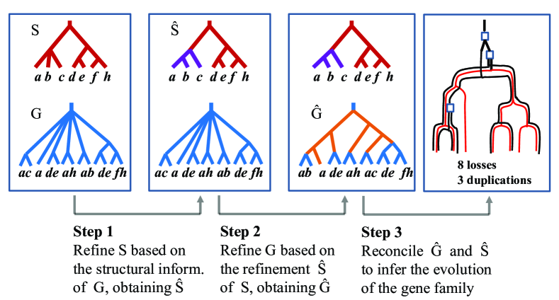
Figure 1: A schematic view of our method for reconciling a non-binary gene tree $G$ of a gene family and a non-binary species tree $S$.

6.3 A Heuristic Reconciliation Method

Since the general reconciliation problem is NP-hard, it unlikely has a polynomial-time algorithm. An efficient heuristic method for it is developed here.

As illustrated in Fig. 1, the method consists of three steps. Given an arbitrary gene tree $G$ of a gene family and the containing species tree $S$, our method first computes a binary refinement $\hat{S}$ of $S$ using the structural information of $G$; it then computes a binary refinement $\hat{G}$ of $G$ based on $\hat{S}$ in the second step; finally, it outputs a hypothetical duplication history of the gene family by reconciling $\hat{G}$ and $\hat{S}$.

Reconciliation of a binary gene tree and a binary species tree is well studied. We shall only describe the detail of the first and second steps in the rest of this section.

6.4 Step One: Resolve Non-binary Species Tree Nodes

Our algorithm for resolving non-binary species tree nodes is motivated by the following facts. Recall that the lca reconciliation map is denoted by $\lambda$. Assume the input gene and species trees be $G$ and $S$, respectively, where $G$ may not be binary. We resolves the non-binary nodes in $S$ one by one.

Consider a non-binary node $s\in S$ having children $s_{1},s_{2},\cdots,s_{n(s)}$, where $n(s)\geq 3$. We define the preimage set

$$\mbox{Pre}(s)=\{g\in V(G):\lambda(g)=s\}$$

of $s$ under $\lambda$. Then, $\mbox{Pre}(s)$ has the following properties:

• For each $g\in\mbox{Pre}(s)$, there are at least two children $s_{i}$ and $s_{j}$ of $s$ such that

  $$L(g)\cap L(s_{i})\neq\phi,\;L(g)\cap L(s_{j})\neq\phi.$$

  In other words, some descendants of $g$ are found in modern species evolving from $s_{i}$, whereas some other descendants of $g$ are found in those evolving from $s_{j}$.

• For each $g\in\mbox{Pre}(s)$ and a child $g^{\prime}$ of $g$, if $g^{\prime}\not\in\mbox{Pre}(s)$, there exist $s_{j}$ such that $g^{\prime}$ is mapped to $s_{j}$ or a node below it.

To resolve the non-binary node $s$, we need to replace the star tree consisting of $s$ and its children with a rooted binary tree $T_{s}$ with root $s$ and $n(s)$ leaves each labeled by a unique $s_{i}$, $1\leq i\leq n(s)$. It is well known that $T_{s}$ has an equivalent partial partition system

$${\mathcal{P}}(T_{s}) = \{[L(u_{1}),L(u_{2})]:u_{1}\mbox{ and }u_{2}\mbox{ are siblings in }T_{s}\}$$

over $\{s_{1},s_{2},\cdots,s_{n(s)}\}$. The partition corresponding to the children of the root of $T_{s}$ is called the first partition. We construct ${\mathcal{P}}(T_{s})$ through computing the first partition recursively. Therefore, we resolve $s$ by recursively solving the so-called minimum duplication bipartition problem (Ourangraoua et al., 2011). We take this approach for two purposes. First, it may reduce the overall duplication cost. Second, pushing duplication down in the species tree can also reduce the gene loss cost even if the resulting reconciliation is not optimal in terms of the duplication cost.

Consider a binary refinement $T_{s}$ of $s$. By definition, it is a binary tree over $s_{i}$ ($1\leq i\leq n(s)$). Let its first partition be $[A,B]$, which is the partition of the set $\{s_{1},s_{2},\cdots,s_{n(s)}\}$. For a gene tree node $g\in\mbox{Pre}(s)$ with two children $g_{i}$ ($1\leq i\leq 2$), $g$ is associated with a duplication occurring before the root of the refinement if and only if $L(g_{i})\cap A\neq\phi$ and $L(g_{i})\cap B\neq\phi$ for some $i$. Hence, $g$ is not associated with a duplication occurring before the root of $T_{s}$ (or before $s$ in $S$) if and only if $g$ is mapped to a node below the root or $g$ is mapped to the root, but its children are mapped below the root. If the former is true, $L(g)=L(g_{1})\cup L(g_{2})\subseteq A$ or $L(g)\subseteq B$. If the latter is true, $L(g_{1})\subseteq A$ and $L(g_{2})\subseteq B$ or vise versa. Hence, $g$ is not associated with a duplication occurring before the root if and only if

$$L(g_{1})\subseteq A\mbox{ or }L(g_{1})\subseteq B,$$ (1)

and

$$L(g_{2})\subseteq A\mbox{ or }L(g_{2})\subseteq B.$$ (2)

The last statement can also be generalized to non-binary gene tree nodes. In the rest of this discussion, for clearance, we call $L(g_{1})|L(g_{2})$ a split rather than a partial partition.

Motivated by this fact, we propose to find the first partition that maximizes the splits $L(g_{1})|L(g_{2})|\cdots|L(g_{k})$ that satisfy the generalization of the conditions Eqn. (1)-(2), where the nodes $g_{i}$ are the children of some internal node in the gene tree. Formally, for a partial partition $[P,Q]$, we say that it does not cut a multiple split $A_{1}|A_{2}|\cdots|A_{k}$ in the gene tree if and only if for every $i$,

$$A_{i}\cap P=\phi,\;\;\mbox{ or }A_{i}\cap Q=\phi.$$ (3)

The algorithm for finding the first partition is summarized below. Recall that we refine a non-binary node $s$ and its children by recursively calling the first partition algorithm.

First Partition Algorithm

${\mathcal{S}}=\phi$; /* It is used to keep partitions */

For each $i$

FirstExtension($[\{i\},\phi]$, $\mathcal{S}$);

Output the best partition in $\mathcal{S}$;

FirstExtension($[P,\phi]$, $\mathcal{S}$) $\{$

1. For each $i\not\in P$

Compute $n(i)$, the # of the gene tree splits not cut by $[P,\{i\}]$;

2. Select $j$ such that $n(j)=\max_{i}n(i)$;

3. If $P\cup\{j\}\neq L(S)$ do {

SplitExtension($[P,\{j\}]$, ${\mathcal{S}}$); FirstExtension($[\{j\}\cup P,\phi]$, ${\mathcal{S}}$);

$\}$ else

Add $[P,\{j\}]$ into $\mathcal{S}$;

$\}$ /* End of FirstExtension */

SplitExtension($[P,Q]$, $\mathcal{S}$) ${\bf\{}$

1. For each $i\not\in P\cup Q$

Compute $n_{1}(i)$, the # of the gene tree splits not cut by $[P,Q\cup\{i\}]$;

Compute $n_{2}(i)$, the # of the gene tree splits not cut by $[P\cup\{i\},Q]$;

2. Select $j$ such that $\max\{n_{1}(j),n_{2}(j)\}=\max_{i}\{n_{1}(i),n_{2}(i)\}$;

3. If ($P\cup\{j\}\neq L(S)$) do $\{$

SplitExtension($[\{j\}\cup P,Q]$, $\mathcal{S}$) if $n_{1}(j)\geq n_{2}(j)$;

SplitExtension($[P,Q\cup\{j\}]$, $\mathcal{S}$) if $n_{2}(j)>n_{1}(j)$;

$\}$ else $\{$

Add $[\{j\}\cup P,Q]$ into $\mathcal{S}$ if $n_{1}(j)\geq n_{2}(j)$;

Add $[P,Q\cup\{j\}]$ into $\mathcal{S}$ if $n_{2}(j)>n_{1}(j)$;

$\}$

$\}$ /* End of SplitExtension */

The First Partition (FP) algorithm is illustrated with an example in Fig. 2, where the computation flow of the subprocedure FirstExtension($\{c\}$, $\phi$) is outlined. In this example, we try to resolving a non-binary species tree node with six children $a,b,c,d,e,f$ using the splits in the gene tree. The gene tree splits are used in the step 1 of both FirstExtension( ) and SplitExtension( ) and not listed explicitly here. After partial partition $[\{c\},\{f\}]$ is obtained, the SplitExtension( ) is called to extend $[\{c\},\{f\}]$ into a partition $[\{c,e,b,d\},\{f,a\}]$ of the child set. Since the computation of the FirstExtension() is heuristic, the partition $[\{c,e,b,d\},\{f,a\}]$ expanded from $[\{c\},\{f\}]$ might not be the optimal first partition of the child set and hence the FirstExtension() is called on $[\{a,f\},\phi]$ to obtain better partitions in the case that $[\{c\},\{f\}]$ does not lead to the optimal first partition. By the same reason, the FirstExtension() is recursively called during computation. Overall, the subprocedure FirstExtension() is recursively called five times, outputing the following partial partitions (in red box in Fig. 2):

$$[\{c\},\{f\}],[\{c,f\},\{b\}],[\{c,f,b\},\{d\}],$$

$$[\{c,f,b,d\},\{a\}],[\{c,f,b,d,a\},\{e\}];$$

and the SplitExtension() is called on these partial partitions to produce the five partitions listed in the bottom (in green). Then, the algorithm selects the best from these obtained partitions.

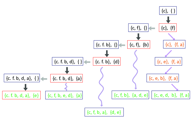
Figure 2: Illustration of the execution of the FirstExtension($\{c\}$, $\phi$). Here, the considered non-binary species tree node has children $a,b,c,d,e,f$. The subprocedure FirstExtension() is recursively executed five times, generating partial partitions (in red) $[\{c\},\{f\}]$, $[\{c,f\},\{b\}]$, $[\{c,f,b\},\{d\}]$, $[\{c,f,b,d\},\{a\}]$, and $[\{c,f,b,d,a\},\{e\}]$, respectively. The SplitExtension() is called on each of these partial partitions to produce the five partitions shown in green in bottom. Here, the geen tree information is omitted.

In general, assume the non-binary species tree node $s$ under consideration has $n(s)$ children and $k^{\prime}$ gene tree nodes are mapped to $s$. The FP algorithm calls recursively the FirstExtension( ) $n(s)-1$ times. During each call of FirstExtension( ), a partition candidate is generated by calling the SplitExtension( ). When the SplitExtension() is executed, whether a split associated with a gene tree node is cut by a partial partition or not is determined by verifying Eqn. (3) with at most $O(k^{\prime})$ set operations. Since the SplitExtension is recursively called at most $n(s)$ times, the First Partition algorithm has time complexity $O(n(s)^{2}k^{\prime})$. Since $n(s)$ is usually small, the algorithm runs fast.

The performance of the FP algorithm is evaluated on randomly generated data and summarized in Table 6.4. Our simulation has two parameters: $c$, the number of the leaf species below the non-binary species tree node to be resolved, and $c_{s}$, the number of splits found in the gene tree. We considered eight combinations of $c$ and $c_{s}$. For each combination, we generated 1000 datasets, giving 8000 datasets in total. For each dataset, we ran the FP method and checkted if it outputted a partition that has the maximum number of non-cut splits or not. Here, the maximum number of splits not cut by an optimal partition was obtained by exhaustive search for each dataset. We also compared the FP algorithm with another reported in (Ouangraoua et al., 2011). It is based on an algorithm for the unweighted hypergraph min cut problem in (Mak, 2011) and can be used for the same purpose. We call it the HC algorithm. Our tests indicate that the FP algorithm outperforms the HC algorithm usually.

Performance of the First Partition (FP) algorithm and an algorithm presented in (Ouangraoua et al., 2011). One thousand random datasets were generated for each combination of $c$ and $c_{s}$, which are the number of leaf species below the non-binary species tree node to be refined and the number of splits found in the input gene tree, respectively. An algorithm made an error if it did not output an optimal partition that induces the smallest number of first duplications. An entry in the last two columns indicates how many times the corresponding algorithm did not output an optimal partition in 1000 tests. # of elements ($c$) # of splits ($c_{s}$) # of errors for FP $\#$ of errors for HC 5 5 7 15 10 0 18 10 5 0 4 10 1 2 20 0 0 15 7 0 3 15 0 1 30 0 1

Putting all the refinements at non-binary species tree nodes together, we obtain a binary refinement $\hat{S}$ of the species tree.

6.5 Step Two: Resolve Non-binary Gene Tree Nodes

When the second step starts, a binary refinement $\hat{S}$ of the species tree $S$ has been obtained. In the second step, our goal is to find a binary refinement $\hat{G}$ of $G$ by resolving every non-binary node in $G$ using $\hat{S}$ such that $\hat{G}$ has the smallest duplication cost when $\hat{G}$ and $\hat{S}$ are reconciled. Moreover, the reconciliation of $\hat{G}$ and $\hat{S}$ also has the optimal loss cost over all the reconciliations with the optimal duplication cost (Theorem 6.3). In the rest of this subsection, we present a linear time algorithm for this step.

We shall refine each non-binary internal node in $G$ separately using the lca reconciliation map $\lambda$ from $G$ to $\hat{S}$ and then combine all the binary refinements to obtain $\hat{G}$. Consider a non-binary internal node $g$ in $G$. Let $g$ have $k$ children $g_{1},g_{2},\cdots,g_{k}$, where $k\geq 3$. We first set

$$I(g)=\{s:\lambda(g_{i})\leq s\leq\lambda(g)\mbox{ for some }i\}.$$

Note that $I(g)$ is a subset of nodes in $\hat{S}$. Furthermore, $I(g)$ forms a subtree rooted at $\lambda(g)$ as shown in Fig. 3C. For simplicity, we also use $I(g)$ to represent the resulting subtree. It is easy to see that in $I(g)$ each leaf is the image of some $g_{i}$ under $\lambda$. However, $I(g)$ may not be a binary subtree because some internal nodes may have a child not belonging to $I(g)$ as shown in Fig. 3C. We use $I^{+}(g)$ to denote the binary tree obtained by including all the children of the non-leaf nodes of $I(g)$. For each species tree node $x$ in the subtree $I^{+}(g)$, we define $\omega(x)$ to be the number of children that are mapped to $x$ under the lca reconciliation $\lambda$. We further define $m(x)$ for each $x\in I^{+}(g)$ as

$$m(x)=\left\{\begin{array}[]{ll}\omega(x)&\mbox{if $x$ is a leaf of $I^{+}(g)$,}\\ \omega(x)+\max(m(x_{1}),m(x_{2}))&\mbox{otherwise,}\end{array}\right.$$

where $x_{1}$ and $x_{2}$ are the children of $x$ if $x$ a non-leaf node of $I^{+}(g)$, a subtree of $\hat{S}$. The computation of $m(\;)$ is illustrated in Fig. 3C.

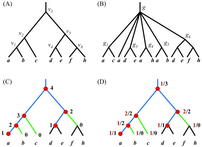
Figure 3: An example of computing $m(\;),\alpha(\;),\beta(\;)$ for a gene tree and a species tree. (A) A binary species tree $\hat{S}$ over 7 species $a,b,c,d,e,f,h$. (B) A gene tree $G$ with a non-binary root $g$. (C) The subtree $I(g)$ (drawn in blue) and $I^{+}(g)$ of $\hat{S}$ in which the number $m(x)$ written beside each node $x$. The lca reconciliation map $\lambda$ from $G$ to $\hat{S}$ maps $g_{1}$ to $v_{2}$, $g_{2}$(which is a leaf) to the left child of $v_{1}$, $g_{3}$ to $v_{4}$, $g_{4}$ to $v_{3}$, $g_{5}$ to $v_{1}$, and $g_{6}$ to $v_{5}$, respectively. $I(g)$ contains $v_{i}$($1\leq i\leq 5$) and the left child of $v_{1}$, which are highlighted in red dot. $I^{+}(g)$ is obtained from $I(g)$ by adding the right child of $v_{1},v_{2}$ and $v_{5}$. The edges in $I^{+}(g)$ but not in $I(v)$ are in green. (D) The $\alpha(u)$ and $\beta(u)$ are given in the format of $\alpha(u)$/$\beta(u)$ for each $u$, from which three duplications and three gene losses are inferred for refining the non-binary node $g$.

Theorem 6.2.

At least $m(\lambda(g))-1$ duplications are required to produce the ancestral genes represented by $g_{1},g_{2},\cdots,g_{k}$

Proof. Consider the partial order set (poset)

$${\mathcal{O}}=(\{L(\lambda(g_{i})):1\leq i\leq k\},\subseteq),$$

in which an element corresponds to the image of some child of $g$ and the binary relation is subset inclusion. Clearly, $m(\lambda(g))$ is the size of the longest chain in $\mathcal{O}$. A subset ${\mathcal{A}}$ of $\mathcal{O}$ is an antichain if for any $x,y\in{\mathcal{A}}$, $x$ and $y$ are not comparable, i.e., $x\not\subseteq y$ and $y\not\subseteq x$. For any $i\neq j$, if $L(\lambda(g_{i}))$ and $L(\lambda(g_{j}))$ are not comparable, they are disjoint since they correspond to two different nodes of $I^{+}(g)$, a subtree of the species tree. Hence, an antichain consists of disjoint elements in $\mathcal{O}$. Let $M$ be the smallest number of antichains into which $\mathcal{O}$ may be partitioned. In (Berglund et al., 2006) (see also (Chang and Eulenstein, 2005)), it is proved that $M-1$ is a lower bound on the number of duplications needed to produce $g_{1},g_{2},\cdots,g_{k}$. By a dual of Dilworth’s theorem (Mirsky, 1971), $M$ is equal to $m(\lambda(g))$, the size of the longest chain. $\Box$

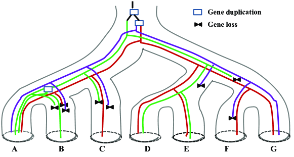
Figure 4: A schematic view of the inferred evolution of the gene family in the containing species tree in the example given in Fig. 3. (A) The binary refinement of the gene tree obtained from resolving the non-binary root $g$. (B) A ‘full’ reconciliation of the gene tree and species tree, which is obtained from reconciling the obtained binary refinement of the binary refinement of the gene tree (in (A)) and the given species tree.

Consider a hypothetical evolution of a gene family in the containing specie tree as shown in Fig. 4. In the species tree, branches represent species. There are two numbers associated with each branch $e$ from $p(u)$ to $u$: the number $\alpha(u)$ of ancestral genes residing in the species represented by $e$ when it just emerged, and the number $\beta(u)$ of ancestral genes in the species just before it speciated into its child species. Clearly, if duplication occurred in the species, $\beta(u)>\alpha(u)$ and their difference is the number of the duplication events that ever occurred, where we assume a duplication event produced one extra gene copy; if there were gene losses, $\alpha(u)>\beta(u)$ and their difference is the number of gene losses. It is easy to see that the values of $\alpha(u)$ and $\beta(u)$ are uniquely determined by the evolution itself. Conversely, each set of such numbers determines uniquely a family of evolutionary histories having the same number of duplication and gene loss events. In the rest of this section, we shall work on these numbers of a partial evolutionary history instead of the evolutionary history itself.

We shall infer a reconciliation with exactly $m(\lambda(g))-1$ duplications associated with $g$. By Theorem 6.2, such a reconciliation has the least duplication events. The inferred duplications are postulated on the different branches of $I^{+}(g)$ to minimize gene losses. To infer these duplications, we define $\alpha(u)$ and $\beta(u)$ for each node $u$ of $I^{+}(g)$ as follows. Because we are working on a partial evolution of the gene family, $\alpha(u)$ and $\beta(p(u))$ are not always equal, but satisfy Eqn. (7) instead.

For the root $r$ of $I^{+}(g)$,

$$\hskip 10.00002pt\alpha(r)=1,$$ (5)

$$\hskip 10.00002pt\beta(r)=\max\{\min\{m(r_{1}),m(r_{2})\},1\}+\omega(r),$$ (6)

where $r_{1}$ and $r_{2}$ are the children of $r$. In general, for a non-root internal node $u$ with parent $p(u)$, a sibling $u^{\prime}$, and children $u_{1}$ and $u_{2}$, we have

$$\alpha(u)=\beta(p(u))-\omega(p(u)),$$ (7)

$$\beta(u)=\left\{\begin{array}[]{ll}m(u),\;\;\;\;\;\;\mbox{if }\alpha(u)\geq m(u)\mbox{ or $u$ is a leaf},\\ \gamma(u),\;\;\;\;\;\mbox{otherwise.}\\ \end{array}\right.$$ (10)

where we define

$$\gamma(u)=\max\{\alpha(u),\min\{m(u_{1}),m(u_{2})\}+\omega(u),1+\omega(u)\}.$$

For the example in Fig. 3, the computation of $\alpha()$ and $\beta()$ is shown in Fig. 3 (D).

If $\alpha(u)<\beta(u)$, we postulate $\beta(u)-\alpha(u)$ duplications in the branch entering $u$; if $\alpha(u)>\beta(u)$, we postulate $\alpha(u)-\beta(u)$ gene losses in the corresponding branch. In total, we postulate $\sum_{u\in I^{+}(g)}\max(\beta(u)-\alpha(u),0)$ duplications and $\sum_{u\in I^{+}(g)}\max(\alpha(u)-\beta(u),0)$ gene losses.

For the example given in Fig. 3, we infer two duplications above the root of the species tree and one duplication in the branch from $v_{2}$ to $v_{1}$ to refine the non-binary root $g$ of the gene tree, resulting in the binary refinement in Fig. 4A. The full reconciliation of the gene tree and the species tree given in Fig. 3 can be obtain by combining the refinement of non-binary root $g$ and inferences at other binary nodes and is shown in Fig. 4B.

Theorem 6.3.

(1) The reconciliation described above requires the least duplications (which is $m(\lambda(g))-1$) for resolving a non-binary node $g$.

(2) It also has the minimum loss cost over all the reconciliations with the optimal duplication cost for resolving $g$.

The full proof of Theorem 6.3 is sophisticated and appears in Section B of the supplementary document. However, its idea is clear. Recall that, the non-binary node $g$ is mapped to the root of $I^{+}(g)$. In the subtree $I^{+}(g)$, by the definition of $m(\;)$, any path from the root $\lambda(g)$ to a leaf contains at most $m(\lambda(g))$ images of the children of $g$; furthermore, there is such a path $P$ containing exactly $m(\lambda(g))$ children images. By calculating $\alpha(u)$ and $\beta(u)$ with formulas (5)-(10), we pushdown duplications from the root as far as possible by postulating a duplication in a branch of $P$ whenever it is necessary. By doing so, we guarantee that the resulting reconciliation has the least gene loss cost while keeping the duplication cost unchanged. For the example given in Fig. 3, $P$ is the leftmost path from the root to the leaf labeled with $a$ in the species tree. We postulate all three duplications along $P$ and three losses off $P$.

By preprocessing the lca map and the species tree $\hat{S}$, we can resolve all the non-binary gene tree nodes in linear time. The detail of linear-time implementation is omitted here.

7 Implementation and Performance Analysis

The algorithms presented above have been implemented in Python. Given an arbitrary rooted gene (family) tree and an arbitrary rooted species tree, which can be binary or non-binary, our reconciliation program outputs a hypothetical duplication history of the gene family. Although our program is heuristic, it usually outputs an evolutionary history having the smallest user-selected reconciliation cost. Our program has the following features.

1. Following (Vernot et al., 2008), our program indicates whether an inferred duplication is required or weakly-supported.

2. For a large gene family, our program may output a set of solutions with the same reconciliation cost.

3. Our program can take a set of arbitrary gene trees and a species tree as its input. When the input includes $k$ gene trees $G_{i}$ ($1\leq i\leq k$) and a species tree, the program attempts to refine all the gene trees and the species tree to minimize the sum of the reconciliation costs $c(S,G_{i})$, where $c$ is the user-selected cost function.

   Recall that a star tree is a rooted tree in which all the leaves are the children of the root and hence any binary tree is a binary refinement of the star tree over the same set of species. Accordingly, our program can be used as a tool for inferring species tree from a set of gene trees if the star tree over the containing species and the set of gene trees are used as input. The performance of our program for species tree inference is assessed in Section 7.2.

4. Our program can be executed from command line to allow for automated analysis of a large number of gene trees.

7.1 Validation Test I: Inferring Tor Gene Duplications

The target of rapamycin (Tor) gene is responsible for nutrient-sensing and highly conserved among eukaryotes. In mammals, the unique mTor governs cellular processes via two distinct complexes Tor Complex1 (TorC1) and TorC2. However, in the budding yeast S. cerevisiae, the fission yeast S. pombe, and other fungal species, there are two Tor paralogs. Moreover, four Tor paralogs have been found in Leishmania major and Trypanosoma brucei, two species of phylum Kinetoplasta (Kinetoplastids).

Shertz et al. (2011) investigated the evolution of the Tor family in the fungal kingdom. They reconstructed the Tor tree over thirteen fungal species (redrawn in Fig. 5A) and from it inferred four duplication events that are responsible for producing two Tor paralogs in fungal kingdom. A whole genome duplication (WGD) event is inferred, occuring in the ancestor of S. cerevisiae approximately one hundred million years ago; S. cerevisiae, S. paradoxus, and other species that descend from the ancestor retained two Tor paralogs. However, three independent lineage-specific duplications are responsible for the two paralogs in S. pombe, B. dendrobatids and P. ostreatus, respectively. When we applied out program to the Tor tree and the non-binary species tree downloaded from the NCBI taxonomy database (drawn in Fig. 5B), the same set of duplications were inferred.

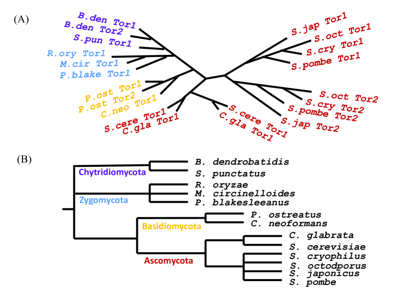
Figure 5: (A) A Tor gene tree over thirteen fungal species, redrawn based on the phylogenetic relationship of the Tor genes reported in (Shertz et al., 2011). (B) A non-binary species tree of the studied fungal species downloaded from the NCBI taxonomy database.

7.2 Validation Test II: Gene Guplications in Drosophila

We further apply our reconciliation program to study gene duplication in the Drosophila species. We used the gene tree data prepared by Hahn (2007). It contains 13376 gene trees over twelve Drosophila species. The 3707 of the gene families contain multiple gene instances in at least one species, whereas the rest are single-gene families. We compared our program with CAFE, a statistical program for duplication inference reported in (Hahn et it., 2005) on the multiple gene families. For each multiple gene family, we first contracted edges having low support value in each gene (family) tree using cut-off value $X$(80, 90, or 100) and ran our program on the resulting gene trees, which may or may not be binary. Our program had similar performance for the three cut-off values. Fig. 6 shows the performance of our program when the cut-off value is set to 80.

We also ran CAFE for the multiple-gene families. Since the duplication inference of CAFE is independent of the family gene tree, the cut-off value used for processing gene trees has no impact on CAFE’s performance.

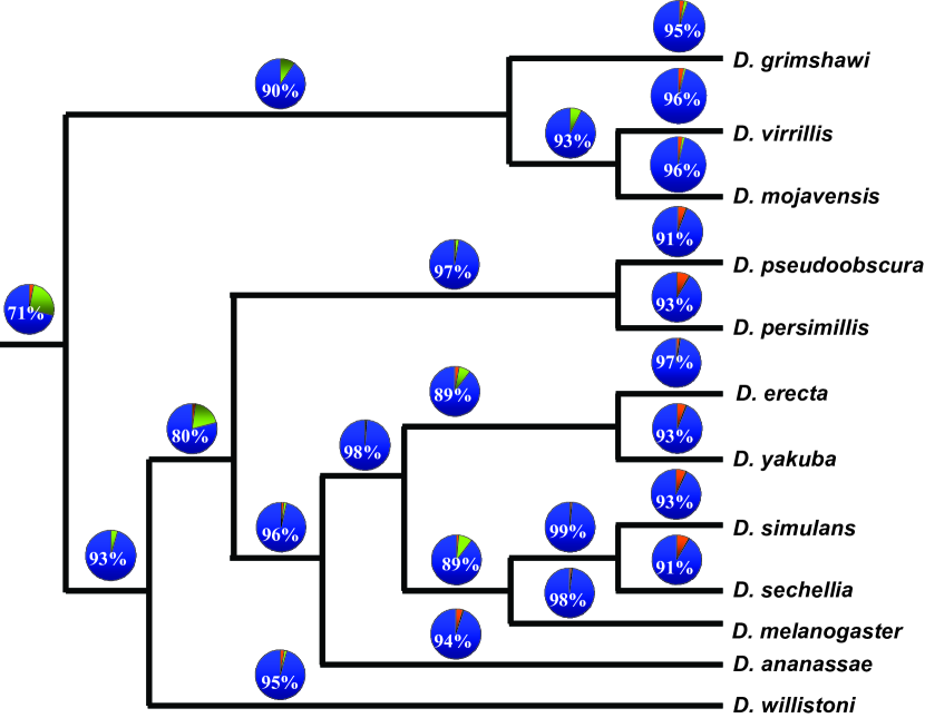
Figure 6: Comparison of our method and CAFE (Hahn et al., 2005) on the Drosophila gene families. The branch lengths are arbitrary in the species tree. In a pie chart, the three sectors represent the proportions of multiple gene families for which both methods infer same duplications (blue, also given in percentage), only CAFE inferred duplications (orange) and only our method inferred duplications (shallow green), respectively.

Except for the root branch and three others, both programs identified the same duplication events for over 90% of multiple gene families. Clearly, our method inferred more duplication events along deep branches, whereas CAFE inferred more along branches ending with a leaf, called informative branches, consistent with the observation made by Hahn (2007). In fact, CAFE often overestimates duplications in the informative branches in our simulation test on the same species tree reported in Section7.3. Hence, combining the both methods should give accurate estimation of the gene duplications occurring on both deep and informative branches in the species tree.

Accuracy of inferring the unrooted Drosophila species tree form unrooted gene trees. Accuracy0: The accuracy of inferring the species tree from original gene trees obtained in (Hahn, 2007); accuracyX: The accuracy of the inference with the non-binary gene trees obtained from the original gene trees via branch contraction with the cut-off value X=60, 90. No. of gene trees Accuracy0(%) Accuracy60(%) Accuracy90(%) 5 21 35 34 10 45 72 54 20 61 87 68 30 76 92 84

When a set of unrooted gene trees (and a star tree) are used as input, our program infers an unrooted binary species tree. We used the Drosophila gene trees to test our program in inferring unrooted species tree. We used the original gene trees and the classes of non-binary gene trees obtained from branch contraction with cut-off value 60 and 90. From the results given in Table 7.2, we observe that contracting weakly supported edge (with support value below 60%) improves greatly the accuracy of inferring unrooted species tree. It is also true that contracting high-supported branches reduces the accuracy of inferring species tree.

7.3 Validation Test III: Simulation

We assess both the CAFE and our method for gene duplication inference through random simulation on the same Drosophila species tree as used in Section 7.2. The twelve species covered in the species tree have evolved from their least common ancestor in the past roughly 63 million years (Hahn, 2007). We generated 1000 random gene families in the birth-death model by setting both duplication and loss rates to 0.002 per million years, which are estimated from the gene evolution in the species tree (Hahn et al., 2005). Each random gene family includes a small number of instances in a species. For each gene family, we recorded gene duplication and loss events occurring along every branch of the species tree; we then derived its gene tree from the recorded duplication events.

From the true tree of a random gene family, we also derived two approximate gene trees by contracting branches that are shorten than 2 and 3 million years, respectively. The resulting trees may or may not be binary for each gene family. We ran our program to infer duplication events by reconciling each of the three obtained trees and the species tree for each gene family. We then computed the accuracy of our program for duplication inference in each of the three cases. Recall that the CAFE program infers gene duplication events without using gene tree information. For each gene family, we simply ran the CAFE program using the same duplication and loss rates 0.002 per million years and computed its accuracy.

The performance of the two programs is summarized in a table in the Section C of the supplementary document. As a reconciliation method, our program uses the structural information of a gene tree to infer gene duplication and thus tends to overestimate duplication events along deep branches. In our test, it inferred correctly the duplication history from the true gene tree for all except for one gene families. When the trees obtained from edge contraction were used, our program overestimated duplications frequently. But it still has high accuracy to detect duplications on both deep and informative branches. In contrast, the CAFE program often overestimated duplications along the informative branches. We noticed that it also overestimated duplications on the root branch (the first branch in the table). The reason for this fact is unclear.

Additionally, we used the same simulated data to evaluate the accuracy of the binary refinement of the input non-binary species tree. Here, we assume the species tree is correctly rooted. We contracted the branches shorter than 10 million years in the species tree, obtaining the following non-binary tree (in Newick format):

((dgri,dmoj,dvir),dwil,(dpse,dper),(dmel,dsec,dsim,dere,dyak,dana)).
The accuracy analysis is reported in Table 7.3. When a set of true gene trees was used, the program could output the true species tree as the binary refinement of the above non-binary species tree. When a set of contracted gene trees was used, the program also performed well. For example, with more than 15 gene trees derived from contracting about 3 edges, our program could recover the true species tree from the non-binary species tree given above with accuracy over 97%.

Accuracy of the binary refinement of the input non-binary species tree. The accuracy is given in percentage of the cases for which the program outputted the Drosophila species tree as the binary refinement of the non-binary input tree (over 100 tests for each entry in the table). $N$ is the number of input gene trees; A is the accuracy of the output binary refinement. $N$ Contraction rate A(%) Mean no. of removed edges Max. node degree 2 0.1 65 1.03 2.79 5 95 0.97 2.73 10 100 0.99 2.75 15 100 1.03 2.75 20 100 0.99 2.72 30 100 0.99 2.73 2 0.3 26 2.98 3.82 5 72 2.91 3.73 10 90 2.95 3.78 15 97 2.90 3.75 20 99 2.95 3.77 30 100 2.99 3.80 2 0.5 7 4.84 5.03 5 27 4.83 4.96 10 65 5.00 5.14 15 66 4.94 5.09 20 76 4.91 5.01 30 90 5.02 5.08

8 Discussion

We have been investigated the general reconciliation problem, in which both input gene and species trees can be non-binary. Only special cases of this problem had been studied in literature. When the input species tree is binary and the input gene tree is non-binary, the reconciliation problem is polynomial-time solvable through a dynamic programming approach (Chang and Eulenstein, 2006; Durand et al., 2005). However, if the input species tree is non-binary, the problem becomes much more hard. Vernot et al. (2008) developed a heuristic method for this case.

In this paper, we approach the general reconciliation problem via finding the binary refinements of gene tree and species tree that minimize a reconciliation cost. Such an approach is promising as it unifies gene duplication inference through tree reconciliation with inferrng species tree from gene trees.

First, we have proved that the general reconciliation problem is NP-hard even for the duplicaiton cost. This answers an open problem on tree reconciliation (Eulenstein et al., 2010; Vernot et al., 2008). It suggests that the general reconciliation problem is unlikely polynomial time solvable.

We then present a fast heuristic algorithm to solve the general reconciliation problem. Given a gene tree $G$ and a species tree $S$, we reconcile $G$ and $S$ in two steps. In the first step, a binary refinement $\hat{S}$ of $S$ is computed using the structural information of $G$ if $S$ is non-binary. We have presented a novel algorithm for the purpose. The algorithm for the minimum duplication speciation problem given in Ourangaoua et al. (2011) can be used in this step. However, our validation test shows that our proposed algorithm outperforms theirs. This step will not be executed if $S$ is a binary tree.

In the second step, a binary refinement $\hat{G}$ of $G$ is computed using $\hat{S}$ if $G$ is not binary. We have developed a linear-time algorithm for this step. Our algorithm benefits from an elegant theorem in order theory (Mirsky, 1971). We focus on the longest chain instead of disjoint partitions of the images of the children of a non-binary node in $G$ (Berglund et al., 2006; Chang and Eulenstein, 2006). Our method outputs a reconciliation with the optimal duplication cost. Moreover, it has the smallest gene loss cost over all reconciliations with the optimal duplication cost. When two binary trees are reconciled, the lca reconciliation has not only the best duplication cost (Gorecki and Tiuryn, 2006), but also the optimal gene loss cost (Chauve and El-Mabrouk, 2009). However, such a reconciliation simply does not exist for non-binary gene trees. Our proposed algorithm for resolving non-binary gene tree nodes is identical to the standard duplication inference procedure when applied to binary gene tree nodes. Thus, our algorithm can be considered as a natural generalization of the standard reconciliation to non-binary gene trees. In our implemented program, the user can also choose the dynamic programming algorithm proposed by Durand et al. (2005) to refine the non-binary gene tree in the second step.

Our algorithm has been implemented into a computer program which is online available to evolutionary biology community. A tree reconciliation method often overestimates duplication events along a deep branch in the input species tree (Hahn, 2007). First, such a method takes into account both gene copies in extant species and gene tree structure. When gene tree and the containing species tree are inconsistent at an internal tree node, duplication has to be assumed. Therefore, a deep coalescence could lead to overestimation of gene duplication events along the branch where the deep coalescence event occurred. However, our preliminary study suggests that the effect of deep coalescence on gene duplication inference is not as severe as previously thought. Secondly, deep branches in both gene and species trees are often reconstructed with low support value because of artifacts caused by low taxon sampling or long branch attraction (Koonin, 2010). Any error occurring in deep branch estimation might lead to overestimation of duplications along an incorrectly-inferred deep branch. Our method attempts to reduce the error of the second type by reconciling non-binary gene and species trees.

Probabilistic approaches assume that gene duplication and loss events are neutral processes and provide a natural setting for incorporating sequence evolution directly into the reconciliation process (Akerborg et al., 2009; Arvestad et al., 2004; Arvestad et al., 2009; Gorecki and Eulenstein, 2011), but they are computation and data intensive. Our approach is based on parsimony principle and thus better suited to data sets where gene evolution events are rare. Hence, our method is complement to the probability-model-based approach. For instance, the CAFE program often overestimated duplications in informative branches, while our program is quite accurate on them.

Finally, our method for refining non-binary species tree can actually be used for reconstructing species trees from a set of gene trees. Different heuristic methods for species tree inference have been proposed recently (Than and Nakhleh, 2009; Liu and Pearl, 2007). Our experimental test indicates that our proposed method is quite promising for this purpose. It is interesting to explore our approach for species tree inference further in future.

References

- Akerborg et al., (2009) Akerborg, O. et al. (2009) Simultaneous Bayesian gene tree reconstruction and reconciliation analysis. Proc Natl Acad Sci USA 106:5714-5719.
- Arve, (2004) Arvestad, L. et al. (2004) Gene tree reconstruction and orthology analysis based on an integrated model for duplications and sequence evolution. In Proc. of RECOMB’04, pp.326-335.
- Arv, (2009) Arvestad, L., Lagergren, J., Sennblad, B. (2009) The gene evolution model and computing its associated probabilities. J. ACM 56:1-44.
- Bansal, (2010) Bansal, M.S., Shamir, S. (2010) A note on the fixed parameter tractability of the gene-duplication problem. IEEE/ACM Trans. Comput. Biol and Bioinform. 8: 848-850.
- Berglund, (2006) Berglund-Sonnhammer, A, et al. (2006) Optimal gene trees from sequences and species trees using a soft interpretation of parsimony. J. Mol. Evol. 63: 240–250.
- Chang, (2006) Chang, W.C., Eulenstein, O. (2006) Reconciling gene trees with apparent polynomies. In Proc. of COCOON (eds: DZ Chen and DT Lee), LNCS, vol. 4112, pp. 235–244.
- Chauve, (2009) Chauve, C., El-Mabrouk, N. (2009) New perspectives on gene family evolution: losses in reconciliation and a link with supertrees. In Proc. of RECOMB’09, pp. 46-58.
- Chen, (2000) Chen, K., Durand, D., Farach-Colton, M. (2000), NOTUNG: a program for dating gene duplications and optimizing gene family trees. J Comput. Biol. 7:429-447.
- Durand, (2008) Durand, D., Halldorsson, B., Vernot, B. (2005) A hybrid micro- macroevolutionary approach to gene tree reconstruction. J Comput. Biol. 13(2):320–335.
- Eulen, (2010) Eulenstein, O., Huzurbazar, S., Liberles, D. (2010) Reconciling Phylogenetic Trees, In Evolution After Duplication (eds: K. Dittmar and D. Liberles), pp 185–206. Wiley-Blackwell, New Jersey, USA.
- Fitch, (1970) Fitch, W.M. (1970) Distinguishing homologous from analogous proteins. Syst. Zool. 19:99-113.
- Goodman, (1979) Goodman, M. et al. (1979) Fitting the gene lineage into its species lineage, a parsimony strategy illustrated by cladograms constructed from globin sequences. Syst. Zool. 28:132-163.
- Gorecki, (2006) Górecki, P., Tiuryn, J. (2006) DLS-trees: a model of evolutionary scenarios. Theoret. Comput. Sci. 359:378-399.
- Gor, (2011) Górecki, P., Burleigh, G.J., Eulenstein, O. (2011) Maximum likelihood models and algorithms for gene tree evolution with duplications and losses. BMC Bioinform. 12(Suppl 1):S15.
- Hahn et al, (2005) Hahn, M.W. et al. (2005) Estimating the tempo and mode of gene family evolution from comparative genomic data. Genome Res. 15:1153-1160.
- Hahn, (2007) Hahn, M. (2007) Bias in phylogenetic tree reconciliation methods: implications for vertebrate genome evolution. Genome Biol. 8(7):R141
- Hudson, (1990) Hudson, R. (1990) Gene genealogies and the coalescent process. In Oxford Surveys in Evolutionary Biology, vol. 7, pages 1-44. Oxford University Press.
- Koonin, (2010) Koonin, E.V. (2010) The origin and early evolution of eukaryotes in the light of phylogenomics. Genome Biol. 11: 209.
- Kristensen, (2011) Kristensen, D.M., Wolf, Y.I., Mushegian, A.R., Koonin, E.V. (2011) Computional methods for gene orthology inference. Briefings in Bioinform. 12: 379-391.
- Liu and Pearl, (2007) Liu, L., Pearl, D.K. (2007) Species trees from gene trees: Reconstructing Bayesian posterior distri-butions of a species phylogeny using estimated gene tree distributions. Syst. Biology 56: 504 C514.
- Maddison, (1989) Maddison, W. (1989) Reconstructing character evolution on polytomous cladograms. Cladistics 5:365-377.
- Ma, (2000) Ma, B., Li, M., Zhang, L.X. (2000) From gene trees to species trees. SIAM J. Comput. 30: 729-752. Also in Proc. RECOMB’98, pp. 182-191.
- Mak, (2005) Mak, W.-K. (2005) Faster min-cut computation in unweighted hypergraphs/circuit netlists. In Proc. of 2005 IEEE TSA Int’l Symp. on VLSI, Automation and Test, pp. 67-70.
- Mirsky, (1971) Mirsky, L. (1971) A dual of Dilworth’s decomposition theorem. Amer. Math. Monthly 78:876-877.
- Ouang, (2011) Ouangraoua, A., Swenson, K., Chauve, C. (2011) A 2-Approximation for the minimum duplication speciation problem. J. Comput. Biol. 18:1041-1053.
- Page, (1994) Page, R. (1994) Maps between trees and cladistic analysis of historical associations among genes, organisms, and areas. Syst. Biol. 43:58-77
- Than and Nakhleh, (2009) Than, C., Nakhleh, L. (2009) Species tree inference by minimizing deep coalescences, PLoS Comput. Biol. 5: e1000501. doi:10371/journal.pchi.1000501.
- Vernot, (2008) Vernot, B., Stolzer, M., Goldman, A., Durand, D. (2008) Reconciliation with non-binary species trees. J Comput. Biol. 15(8):981–1006.
- Zhang, (1997) Zhang, L.X. (1997) On a Mirkin-Muchnik-Smith conjecture for comparing molecular phylogenies. J Comput. Biol. 4: 177-187.
- Z, (2001) Zmasek, C., Eddy, S. (2001) A simple algorithm to infer gene duplication and speciation events on a gene tree. Bioinform. 17:821.