Search for $\chi_{c_{J}}(2P)$ from Higher Charmonim E1 Transitions and X,Y,Z States

Abstract

We calculate the E1 transition widths of higher vector charmonium states into the spin-triplet 2P states in three typical potential models, and discuss the possibility to detect these 2P states via these E1 transitions. We attempt to clarify the nature of some recently observed X,Y,Z states by comparing them with these 2P charmonium states in these E1 transitions. In particular, the calculated branching ratios of $\psi(4040),\psi(4160)\to\chi^{{}^{\prime}}_{c_{J}}\gamma$ (J=0,1,2) are found to be in the range of $10^{-4}\mbox{-}10^{-3}$, and sensitive to the 3S-2D mixing of $\psi(4040)$ and $\psi(4160)$. The mixing angle may be constrained by measuring $\psi(4040),\psi(4160)\to Z(3930)\gamma$, if Z(3930) is identified with the $\chi^{{}^{\prime}}_{c_{2}}$ state, and then be used in measuring $\chi^{{}^{\prime}}_{c_{0,1}}$ states. These processes can be studied experimentally at $e^{+}e^{-}$ colliders such as BEPCII/BESIII and CESR/CLEO.

I Introduction

Since the discovery of $J/\psi$ in 1974 Aubert:1974js ; Augustin:1974xw , a lot of charmonium states had been found in the last century. Among them, the vector states $\psi(4040)$, $\psi(4415)$, and $\psi(4160)$, which are commonly assigned as $\psi(3S)$, $\psi(4S)$ and $\psi(2^{3}D_{1})$ respectively, can be directly produced through $e^{+}e^{-}$ annihilation into one photon, and thus can be readily detected at $e^{+}e^{-}$ colliders like BEPCII/BESIII BES2009 and CESR/CLEO.

Aside from these vector resonances themselves, it is also interesting to detect the products via E1 transitions of these vector resonances into lower charmonium states. Especially, the decay channels $\psi(4040,4160,4415)\rightarrow\chi^{{}^{\prime}}_{c_{J}}\gamma,\,J=0,1,2$ can be used to detect the 2P charmonia $\chi^{{}^{\prime}}_{c_{J}}$ and to study the properties of these missing states. The importance of experimental establishment of these 2P charmonia consists in at least two aspects. On one side, the properties of $\chi^{{}^{\prime}}_{c_{J}}$ are important to clarify the calculations in various potential models and coupled-channel models (see, e.g. Li:2009ad and references therein). On the other side, the $\chi^{{}^{\prime}}_{c_{J}}$ could be the candidates of some of the recently observed charmonium-like states, the so-called ”X,Y,Z” states (for a review see e.g. Brambilla:2010cs ).

According to potential model estimates, the spin-triplet 2P states lie between 3.9 and 4.0 GeV in the charmonium family Eichten:1978tg ; Barnes2005 ; Godfrey:1985xj . Experimentally, five charmonium(like) resonances around 3940 MeV have been found recently. The Z(3930) Belle06:Z3930 observed by the Belle Collaboration in 2006 in the $\gamma\,\gamma$ fusion experiment with a mass $3929\pm 5\pm 2$ MeV is identified with the $\chi_{c_{2}}^{{}^{\prime}}$. The X(3915), which was also produced in the $\gamma\,\gamma$ fusion experimentUehara:2009tx and detected in the $J/\psi\,\omega$ channel with a mass about 3915 MeV, is possibly the $\chi_{c_{0}}^{{}^{\prime}}$ Liu:2009fe . The Y(3940) and Y(3915), which were detected in the $B\to J/\psi\omega K$ process by the Belle Collaboration Abe:2004zs and the BaBar Collaboration Aubert:2007vj separately are another candidates for $\chi_{c_{1,0}}^{{}^{\prime}}$. The X(3940), which was found by the Belle Collaboration Belle07:X3940 in the recoiling spectrum of $J/\psi$ in the $e^{+}e^{-}$ annihilation process $e^{+}e^{-}\to J/\psi+X$ and $e^{+}e^{-}\to J/\psi+D\bar{D}^{*}$, seems not to be a 2P state Li:2009zu ; Belle08:X3940&4160 . Another well known state, the X(3872), which was first found in the $J/\psi~{}\pi^{+}\pi^{-}$ invariant mass distribution in the B meson decay around 3872 MeV Belle0309032 with $J^{PC}=1^{++}$, might be interpreted as the $D^{*0}D^{0}+c.c.$ molecule due to the closeness of its mass to the $D^{*0}D^{0}$ threshold. But its large production rate in $p-\bar{p}$ collisions at the Tevatron and some properties seem to support that it could be a compact bound state, such as the 2P charmonium $\chi_{c_{1}}^{{}^{\prime}}$, or a mixture of the $\chi_{c_{1}}^{{}^{\prime}}$ with the $D^{*0}D^{0}+c.c.$ molecule, despite of its lower mass. In fact, the mass of $\chi_{c_{1}}(2P)$ can be lowered to below 3.9 GeV if the color screening effects and coupled channel effects are considered Li:2009zu ; Li:2009ad . So it is interesting to examine in the E1 transitions of higher charmonia if the X(3872) can be seen by having the $\chi_{c_{1}}^{{}^{\prime}}$ component in its wave function.

Because of the phenomenological importance of the $\chi_{cJ}^{\prime}$ states mentioned above, we will study the production of these states in the E1 transitions of higher vector charmonia, say, $\psi(4040)$, $\psi(4160)$ and $\psi(4415)$. The E1 transition width can be estimated by potential models. Various potential models predict various transition widths. However, the transition widths of $\psi(4415)\rightarrow\chi_{c_{J}}^{{}^{\prime}}\,\gamma$ are usually small because of the smallness of the overlap integral between the wave functions of 4S and 2P states. On the other hand, the transition widths of $\psi(4040,4160)\rightarrow\chi_{c_{J}}^{{}^{\prime}}\,\gamma$, are relatively large (tens to hundreds of KeV as those shown in Table 1 and Table 2) and the corresponding branching ratios are about $10^{-4}-10^{-3}$. So the $\chi_{c_{J}}^{{}^{\prime}}$ may be detected at the upgraded BEPCII/BESIII through these channels. Note that the E1 transition width depends on the phase space which is determined by the mass of $\chi_{c_{J}}^{{}^{\prime}}$. Since the $\chi_{c_{2}}^{{}^{\prime}}$ has been identified with Z(3930), we can compare various potential model predictions with the experimental data of $\chi_{c_{2}}^{{}^{\prime}}$ to see if it can be detected in the E1 transitions of higher charmonium states. This comparison may provide some hints in searching for the other two $\chi_{c_{J}}^{{}^{\prime}}$ states.

We introduce three typical potential models in section II, and calculate in section III the E1 transition widths of $\psi(4040,4160,4415)\rightarrow\chi_{c_{J}}^{{}^{\prime}}\,\gamma$ with both lowest- and first-order wave functions in the non-relativistic expansion within these models. We discuss the possibility for producing $\chi_{c_{J}}^{{}^{\prime}}$ from E1 transitions of higher excited charmonium states and compare them with those ”X,Y,Z” states in section IV, where the effects of S-D mixing of $\psi(4040)$ and $\psi(4160)$ on the E1 transition widths are also considered. A summary is given in section V.

II The potential models

There are many phenomenologically successful potential models in the literature. Among them the Cornell model Eichten:1978tg (here we mark it by Model II) is well known, which describes the charmonium system quite well. However, the predicted masses of higher charmonium states seem to be larger than their experimental values Li:2009zu . A distinct example is the mass of $\chi_{c_{2}}^{{}^{\prime}}$ which is about 40 MeV larger than the experimental value. The screened potential model (see Ref Li:2009zu and references therein)(here we mark it by Model I) was proposed to lower the masses of higher charmonia. So we take it here to estimate the E1 transition production of $\chi_{c_{J}}^{{}^{\prime}}$. The third model we take was proposed by Ding et al. Ding:1985rh ; Ding:1991vu (here we mark it by Model III), in which the Coulomb potential has a running coupling constant. The Hamiltonian in these models have the form of $H=-\frac{\vec{P}^{2}}{m_{c}}+V_{V}(r)+V_{S}(r)$, where $V_{V}(r)$ is vector potential and $V_{S}(r)$ is scalar potential and $m_{c}$ is the mass of charm quark.

The potentials in Model I Li:2009zu are:

$$V_{V}(r)=-\frac{4}{3}\frac{\alpha_{C}}{r},\quad V_{S}(r)=\lambda(\frac{1-e^{-\mu r}}{\mu}),$$ (1)

where $\mu$ is the screening factor which makes the long range scalar part $V_{S}(r)$ become flat when $r\gg\frac{1}{\mu}$ and still linearly rising when $r\ll\frac{1}{\mu}$, $\lambda$ is the linear potential slope, and $\alpha_{C}$ is the coefficient of the Coulomb potential. The model parameters are chosen following Ref Li:2009zu :

$$\alpha_{C}=0.5007,~{}~{}~{}~{}~{}~{}\lambda=0.21GeV^{2},$$

$$\mu=0.0979GeV,~{}~{}~{}~{}~{}~{}~{}m_{c}=1.4045GeV,$$ (2)

where $\alpha_{C}\approx\alpha_{s}(m_{c}v_{c})$ is essentially the strong coupling constant at the scale $m_{c}v_{c}$. Here $\mu$ is the characteristic scale for color screening, and $1/{\mu}$ is about 2 $fm$, implying that at distances larger than $1/{\mu}$ the static color source in the $c\bar{c}$ system gradually becomes neutralized by the produced light quark pair, and string breaking emerges.

The potentials in Model II Eichten:1978tg are:

$$V_{V}(r)=-\frac{4}{3}\frac{\alpha_{C}}{r},\quad V_{S}(r)=\lambda r,$$ (3)

with model parameters taken similar to Ref. Barnes2005 :

$$\alpha_{C}=0.5461,\,\lambda=0.1425GeV^{2},\,m_{c}=1.4794GeV$$

The potentials in Model III Ding:1985rh ; Ding:1991vu are

$$V_{V}(r)=\frac{8\pi}{25}\frac{1}{\mbox{ln}(\Lambda r)}\frac{1-\Lambda r}{1+\Lambda r},\,\,V_{S}(r)=\lambda r\,-\,C,$$ (4)

with parameters

$$\Lambda=0.47GeV,~{}~{}~{}~{}~{}~{}\lambda=0.22GeV^{2},$$

$$m_{c}=1.84GeV,~{}~{}~{}~{}~{}~{}~{}C=-0.975GeV.$$ (5)

The potentials above are used to calculate the lowest-order and the first-order non-relativistic wave functions. For the first-order relativistic corrections to the wave functions, we include the spin-dependent part of $H_{SS}$, $H_{LS}$, $H_{T}$ and the spin-independent part $H_{SI}$ as perturbations.

The spin-spin contact hyperfine interaction is

$$H_{SS}=\frac{2}{3m_{c}^{2}}\vec{S_{1}}\cdot\vec{S_{2}}\bigtriangledown^{2}V_{V}.$$ (6)

For Coulombic vector potential, $\nabla^{2}\,(\frac{1}{r})\propto\delta^{3}(\vec{r})$ which gives too large a mass splitting of $J/\psi-\eta_{c}$, so we make a substitution as in Ref. Barnes2005 for Model I and Model II:

$$H_{SS}=\frac{32\pi\alpha_{C}}{9m_{c}^{2}}\,\tilde{\delta}_{\sigma}(r)\,\vec{S}_{c}\cdot\vec{S}_{\bar{c}}\,,$$ (7)

where $\tilde{\delta}_{\sigma}(r)=(\sigma/\sqrt{\pi})^{3}\,e^{-\sigma^{2}r^{2}}$ and $\sigma=1.362GeV$ in Model I and $\sigma=1.0946GeV$ in Model II.

The spin-orbit term is

$$H_{LS}=\frac{1}{2m_{c}^{2}r}(3V_{V}^{{}^{\prime}}(r)-V_{S}^{{}^{\prime}}(r))\vec{L}\cdot\vec{S},$$ (8)

and the tensor force term is

$$H_{T}=\frac{1}{12m_{c}^{2}}(\frac{1}{r}V_{V}^{{}^{\prime}}(r)-V_{V}^{{}^{\prime\prime}}(r))S_{12},$$ (9)

where $S_{12}=3(\vec{\sigma_{1}}\cdot\hat{r})(\vec{\sigma_{2}}\cdot\hat{r})-\vec{\sigma_{1}}\cdot\vec{\sigma_{2}}$.

The spin-independent part is a bit complicated. We take the form as Ref. Lucha:1991vn :

$$H_{SI} = -\frac{\vec{P}^{4}}{4m_{c}^{3}}+\frac{1}{4m_{c}^{2}}\bigtriangledown^{2}V_{V}(r)$$ (10)

$$-\frac{1}{2m_{c}^{2}}\left\{\left\{\vec{P}_{1}\cdot V_{V}(r)\Im\cdot\vec{P}_{2}\right\}\right\}$$

$$+\frac{1}{2m_{c}^{2}}\left\{\left\{\vec{P}_{1}\cdot\vec{r}\frac{V_{V}^{{}^{\prime}}(r)}{r}\vec{r}\cdot\vec{P}_{2}\right\}\right\},$$

where $\vec{P}_{1}$ and $\vec{P}_{2}$ are momenta of c and $\bar{c}$ quarks in the rest frame of charmonium, respectively, which satisfy $\vec{P}_{1}=-\vec{P}_{2}=\vec{P}$, $\Im$ is the unit second-order tensor, and $\{\{\quad\}\}$ is the Gromes’s notation

$$\{\{\vec{A}\cdot\Re\cdot\vec{B}\}\}=\frac{1}{4}(\vec{A}\vec{B}:\Re+\vec{A}\cdot\Re\vec{B}+\vec{B}\cdot\Re\vec{A}+\Re:\vec{A}\vec{B}),$$ (11)

where $\Re$ is a second-order tensor.

Note that we do not include the contributions from the scalar potential in $H_{SI}$ since it is still unclear how to deal with the spin-independent corrections arising from the scalar potential theoretically.

III E1 transition Widths

E1 transitions of higher excited S- and D-wave charmonium states are of interest here because they can be used to produce and identify P-wave states. For the E1 transition width for charmonium, we use the formula of Ref. Kwong:1988ae :

$$\Gamma_{\rm E1}({\rm n}\,{}^{2{\rm S}+1}{\rm L}_{\rm J}\to{\rm n}^{\prime}\,{}^{2{\rm S}^{\prime}+1}{\rm L}^{\prime}_{{\rm J}^{\prime}}+\gamma)$$

$$=\frac{4}{3}\,C_{fi}\,\delta_{{\rm S}{\rm S}^{\prime}}\,e_{c}^{2}\,\alpha\,|\,\langle f|\,r\,|\,i\rangle\,|^{2}\,{\rm E}_{\gamma}^{3}\,$$ (12)

where E_γ is the emitted photon energy.

The spatial matrix element

$$<f|r|i>=\int_{0}^{\infty}R_{f}(r)R_{i}(r)r^{3}dr\,,$$ (13)

involves the initial and final state radial wave functions, and the angular matrix element $C_{fi}$ is

$$C_{fi}=\hbox{max}({\rm L},\;{\rm L}^{\prime})\;(2{\rm J}^{\prime}+1)\left\{{{{\rm L}^{\prime}\atop{\rm J}}{{\rm J}^{\prime}\atop{\rm L}}{{\rm S}\atop 1}}\right\}^{2}.$$ (14)

We are only interested in initial states with $J^{PC}=1^{--}$, i.e., $\psi(4040)$, $\psi(4415)$ and $\psi(4160)$, since they can be easily produced in $e^{+}e^{-}$ annihilation and can transit into spin-triplet 2P states by emitting a photon.

For the masses of initial and final states used to calculate $E_{\gamma}$ in above three models, we take the central values from PDG(2010) Nakamura:2010zzi if the states are well established experimentally. The mass of $\chi_{c_{0}}^{{}^{\prime}}$ is supposed to be 3915 MeV, while for the mass of $\chi_{c_{1}}^{{}^{\prime}}$ we choose two different values: 3872 MeV and 3915 MeV.

The calculated results with lowest-order wave functions are listed in Table 1. The results of Barnes, et al. Barnes2005 , which are similar to the Model II and the results of Godfrey, et al. Godfrey:1985xj , with a relativized Cornell model, are also listed in Table 1 for comparison. From Table 1, one can see that the widths $\Gamma(\psi(4415)\to\chi_{cJ}^{\prime}\gamma)$, are very small due to large cancelation in the overlap integral between wave functions of 4S and 2P states, and therefore are very sensitive to the model details. On the other hand, the predictions for the widths $\Gamma(\psi(4040,4160)\to\chi_{cJ}^{\prime}\gamma)$ are large and insensitive to model details, resulting in quite steady values in different models.

The results obtained with first-order wave functions are listed in Table 2. From (7-10), one can see that the corrections to the non-relativistic potential involve some derivative terms, which make the potential to be more attractive towards the origin. As a result, the wave functions with relativistic corrections will be thinner than those without relativistic corrections. This effect usually reduces the spatial matrix elements $<f|r|i>$ defined in (13), which can be seen directly by comparison between the results of $\Gamma(\psi(4040,4160)\to\chi_{cJ}^{\prime}\gamma)$ listed in Table 1 and in Table 2. However, the relativistic corrections can also change the node structures of the wave functions of higher exited states, such as $\psi(4415)$, and make the cancelation in the overlap integral between the wave functions of 4S and 2P states more modest, and this can be seen in Table 2. On the other hand, the transition width is proportional to the factor $E_{\gamma}^{3}$, which favors initial states with higher masses. Thus, the decay widths $\Gamma(\psi(4415)\to\chi_{cJ}^{\prime}\gamma)$ listed in Table 2 become larger. But we should mention that these results are not very reliable and are more sensitive to the model details than those of $\Gamma(\psi(4040,4160)\to\chi_{cJ}^{\prime}\gamma)$.

We calculate the E1 transition branching ratios of $\psi(4040)$, $\psi(4160)$, and $\psi(4415)$ with their total width taken from PDG(2010) Nakamura:2010zzi . Since the errors of the total widths are relatively small for these states, we only take the central values of the total widths in calculating the branching ratios and do not consider the errors.

Table 1: E1 transition widths and branching ratios of charmonium states with the lowest-order wave functions in various potential models. The masses and total widths of the initial states used in the calculation are the PDG Nakamura:2010zzi central values, while the masses of the final states in the Model I-III calculations are denoted by the numbers in the parentheses. For comparison, the results of Refs. Barnes2005 and Godfrey:1985xj are also listed.

Process		$<f|r|i>\,(GeV^{-1}$)			$\rm k\,(MeV)$			$\Gamma_{\rm thy}$ (keV)					$Br_{\rm thy}~{}(\times 10^{-4})$
Intial	Final	I	II	III	Ours	Ref.Barnes2005	Ref.Godfrey:1985xj	I	II	III	Ref.Barnes2005	Ref.Godfrey:1985xj	I	II	III	Ref.Barnes2005	Ref.Godfrey:1985xj
$\psi(4040)$	$\chi^{{}^{\prime}}_{c_{2}}(3929)$	-4.9	-4.4	-3.4	109	67	119	74	59	36	14	48	9.3	7.4	4.5	1.8	6.0
	$\chi^{{}^{\prime}}_{c_{1}}(3872)$	-4.9	-4.4	-3.4	164	113	145	151	122	74	39	43	18.9	15.3	9.3	4.9	5.4
	$\chi^{{}^{\prime}}_{c_{1}}(3915)$	-4.9	-4.4	-3.4	122	113	145	63	51	31	39	43	7.9	6.4	3.9	4.9	5.4
	$\chi^{{}^{\prime}}_{c_{0}}(3915)$	-4.9	-4.4	-3.4	122	184	180	21	17	10	54	22	2.6	2.1	1.3	6.8	2.8
$\psi(4160)$	$\chi^{{}^{\prime}}_{c_{2}}(3929)$	5.0	4.6	3.8	218	183	210	12	10	7.3	5.9	6.3	1.2	0.97	0.71	0.57	0.61
	$\chi^{{}^{\prime}}_{c_{1}}(3872)$	5.0	4.6	3.8	271	227	234	355	299	210	168	114	34.5	29.0	20.4	16.3	11.1
	$\chi^{{}^{\prime}}_{c_{1}}(3915)$	5.0	4.6	3.8	231	227	234	219	185	132	168	114	21.3	18.0	12.8	16.3	11.1
	$\chi^{{}^{\prime}}_{c_{0}}(3915)$	5.0	4.6	3.8	231	296	269	292	247	173	483	191	28.3	24.0	16.8	46.9	18.5
$\psi(4415)$	$\chi^{{}^{\prime}}_{c_{2}}(3929)$	-0.013	0.093	-0.028	465	421	446	0.04	2.1	0.2	0.62	15	0.006	0.34	0.03	0.1	2.4
	$\chi^{{}^{\prime}}_{c_{1}}(3872)$	-0.013	0.093	-0.028	515	423	469	0.04	1.7	0.2	0.49	0.92	0.006	0.27	0.03	0.08	0.15
	$\chi^{{}^{\prime}}_{c_{1}}(3915)$	-0.013	0.093	-0.028	477	423	469	0.03	1.4	0.1	0.49	0.92	0.005	0.23	0.02	0.08	0.15
	$\chi^{{}^{\prime}}_{c_{0}}(3915)$	-0.013	0.093	-0.028	477	527	502	0.01	0.45	0.04	0.24	0.39	0.002	0.07	0.006	0.04	0.06

Table 2: E1 transition widths and branching ratios of charmonium states in various potential models with the first-order wave functions. The masses and total widths of the initial states used in the calculation are the PDG Nakamura:2010zzi central values, while the masses of the final states in the Model I-III calculations are denoted by the numbers in the parentheses.

Process		$<f|r|i>\,(GeV^{-1}$)			$\rm k\,(MeV)$	$\Gamma_{\rm thy}$ (keV)			$Br_{\rm thy}~{}(\times 10^{-4})$
Initial	Final	$I^{{}^{\prime}}$	$II^{{}^{\prime}}$	$III^{{}^{\prime}}$		$I^{{}^{\prime}}$	$II^{{}^{\prime}}$	$III^{{}^{\prime}}$	$I^{{}^{\prime}}$	$II^{{}^{\prime}}$	$III^{{}^{\prime}}$
$\psi(4040)$	$\chi^{{}^{\prime}}_{c_{2}}(3929)$	-4.3	-3.9	-3.1	109	56	47	29	7.0	5.9	3.6
	$\chi^{{}^{\prime}}_{c_{1}}(3872)$	-3.7	-3.4	-2.8	164	88	72	50	11.0	9.0	6.3
	$\chi^{{}^{\prime}}_{c_{1}}(3915)$	-3.7	-3.4	-2.8	122	37	30	21	4.6	3.8	2.6
	$\chi^{{}^{\prime}}_{c_{0}}(3915)$	-3.0	-2.7	-2.5	122	7.9	6.2	5.3	0.99	0.78	0.66
$\psi(4160)$	$\chi^{{}^{\prime}}_{c_{2}}(3929)$	4.3	4.1	3.4	218	9.2	8.2	5.9	0.89	0.80	0.57
	$\chi^{{}^{\prime}}_{c_{1}}(3872)$	3.6	3.4	3.2	271	189	169	147	18.3	16.4	14.3
	$\chi^{{}^{\prime}}_{c_{1}}(3915)$	3.6	3.4	3.2	231	117	105	91	11.4	10.2	8.8
	$\chi^{{}^{\prime}}_{c_{0}}(3915)$	2.7	2.6	2.9	231	89	81	97	8.6	7.9	9.4
$\psi(4415)$	$\chi^{{}^{\prime}}_{c_{2}}(3929)$	-0.42	-0.13	-0.19	465	42	4.1	8.7	6.8	0.66	1.4
	$\chi^{{}^{\prime}}_{c_{1}}(3872)$	-1.1	-0.77	-0.39	515	219	116	30	35.3	18.7	4.8
	$\chi^{{}^{\prime}}_{c_{1}}(3915)$	-1.1	-0.77	-0.39	477	174	92	24	28.1	14.8	3.9
	$\chi^{{}^{\prime}}_{c_{0}}(3915)$	-1.8	-1.4	-0.65	477	164	105	22	26.5	16.9	3.5

IV Discussions On XYZ States

In this section, we fucus on the implication of the results of $Br(\psi(4040,4160,4415)\to\chi_{cJ}^{\prime}\gamma)$ on searching for XYZ states in these channels. The 3S-2D mixing effects of $\psi(4040)$ and $\psi(4160)$ are also considered in details.

IV.1 Z(3930)

The Z(3930) was found by the Belle Collaboration Belle06:Z3930 in the process $\gamma\gamma\rightarrow D\bar{D}$ with

$$M(Z(3930)) = 3929\pm 5\pm 2~{}\mbox{MeV},$$ (15)

$$\Gamma(Z(3930)) = 29\pm 10\pm 2~{}\mbox{MeV},$$ (16)

$$\Gamma_{\gamma\gamma}{\cal B}(Z(3930)\to D\bar{D}) = 0.18\pm 0.05\pm 0.03~{}\mbox{KeV},$$ (17)

and confirmed by the BaBar Collaboration :2010hk with

$$M(Z(3930)) = 3926.7\pm 2.7\pm 1.1~{}\mbox{MeV},$$ (18)

$$\Gamma(Z(3930)) = 21.3\pm 6.8\pm 3.6~{}\mbox{MeV},$$ (19)

$$\Gamma_{\gamma\gamma}{\cal B}(Z(3930)\to D\bar{D}) = 0.24\pm 0.05\pm 0.04~{}\mbox{KeV}.$$ (20)

The production rate and the angular distribution in the $\gamma\gamma$ center-of-mass frame suggest that this state is the previously unobserved $\chi_{c_{2}}^{{}^{\prime}}$ Belle06:Z3930 ; :2010hk . Its mass, however, is about 40-50 MeV larger than the commonly predicted value in the quenched potential model (see, e.g. Barnes2005 ). A lower mass can be obtained by considering the color screening effect described in Model I Li:2009zu in which the predicted mass is 3937 MeV.

Since $Z(3930)$ is established as the candidate of $\chi_{c_{2}}^{{}^{\prime}}$, searching for $Z(3930)$ in the E1 transitions of $\psi(4040,4160,4415)$ is important to further verify this assignment and can also be a good criterion in searching for and identifying other $\chi_{cJ}^{\prime}$ states in these transitions.

From Table 1 and Table 2, we can see the transition width of $\psi(4040)\rightarrow\chi_{c_{2}}^{{}^{\prime}}\,\gamma$ is 36-74 KeV with the lowest-order wave functions and 29-56 KeV with the first-order wave functions in our calculations within Models I-III and in Ref. Godfrey:1985xj . The corresponding branching ratio is 4.5-9.3$\times 10^{-4}$ and 3.6-7.0$\times 10^{-4}$, respectively. The branching ratio of order of $10^{-4}$ is encouraging to detect $\chi_{c_{2}}^{{}^{\prime}}$ in $\psi(4040)$ E1 transitions. Note that the results of Ref. Barnes2005 is notably small than our results. This is mainly because, the mass of $\chi_{c_{2}}^{{}^{\prime}}$ used in Ref. Barnes2005 is larger than ours and the corresponding energy of the emitted photon is much smaller than ours.

The branching ratio of $\psi(4160)\rightarrow\chi_{c_{2}}^{{}^{\prime}}\,\gamma$ is about one-fifth of that of $\psi(4040)\rightarrow\chi_{c_{2}}^{{}^{\prime}}\,\gamma$ but is still close to $1\times 10^{-4}$. The branching ratio of $\psi(4415)\rightarrow\chi_{c_{2}}^{{}^{\prime}}\,\gamma$ is sensitive to the model details. So it is difficulty to predict how large is the branching ratio of $\psi(4415)\rightarrow\chi_{c_{2}}^{{}^{\prime}}\,\gamma$ in potential models.

IV.2 X(3915),Y(3940),Y(3915)

The X(3915) Uehara:2009tx , Y(3940) Abe:2004zs and Y(3915) Aubert:2007vj are all observed in the invariance mass distribution of $J/\psi\,\omega$ in processes

$$\gamma\,\gamma\rightarrow X(3915) \rightarrow J/\psi\,\omega,$$ (21)

$$B\rightarrow K\,Y(3940), Y(3940) \rightarrow J/\psi\,\omega,$$ (22)

$$B\rightarrow K\,Y(3915), Y(3915) \rightarrow J/\psi\,\omega,$$ (23)

with masses

$$M(X(3915)) = 3915\pm 3\pm 2~{}\mbox{MeV},$$ (24)

$$M(Y(3940)) = 3943\pm 11\pm 13~{}\mbox{MeV},$$ (25)

$$M(Y(3915)) = 3914.6^{+3.8}_{-3.4}\pm 2.0~{}\mbox{MeV},$$ (26)

total widths

$$\Gamma(X(3915)) = 17\pm 10\pm 3~{}\mbox{MeV},$$ (27)

$$\Gamma(Y(3940)) = 87\pm 22\pm 26~{}\mbox{MeV},$$ (28)

$$\Gamma(Y(3915)) = 34^{+12}_{-8}\pm 5~{}\mbox{MeV},$$ (29)

and partial widths

$$\Gamma_{\gamma\gamma} \times\,\,\,{\cal B}(X(3915)\to J/\psi\,\omega) =\left\{\begin{array}[]{ll}61\pm 17\pm 8\quad\mbox{eV},&J^{P}=0^{+}\\ 18\pm 5\pm 2\quad\mbox{eV},&J^{P}=2^{+},\mbox{helicity-2}\end{array}\right.$$ (32)

$${\cal B}(B\rightarrow K\,Y(3940)) \times\,\,\,{\cal B}(Y(3940)\rightarrow J/\psi\,\omega) =(7.1\pm 1.3\pm 3.1)\times 10^{-5},$$ (33)

$${\cal B}(B^{+}\rightarrow K^{+}\,Y(3915)) \times\,\,\,{\cal B}(Y(3915)\rightarrow J/\psi\,\omega) =(3.5\pm 0.2\pm 0.4)\times 10^{-4},$$ (34)

$${\cal B}(B^{0}\rightarrow K^{0}\,Y(3915)) \times\,\,\,{\cal B}(Y(3915)\rightarrow J/\psi\,\omega) =(3.1\pm 0.6\pm 0.3)\times 10^{-4}.$$ (35)

Although the differences of masses and total widths of the three signals are within $2\sigma$, especially those of X(3915) and Y(3915) are less than one $\sigma$, it is not clear whether these three signals come from the same particle. BaBar Aubert:2007vj considers Y(3915) and Y(3940) as the same state since the smaller values of both the mass and total width of Y(3915) derived from fitting data by BaBar can partially be attributed to larger data sample used by BaBar, which enable them to use smaller $J/\psi\,\omega$ mass bin in their analysis Yuan:2009iu . Y(3940) and X(3915) are also considered to be the same state in Refs. Uehara:2009tx ; Yuan:2009iu ; Zupanc:2009qc ; Godfrey:2009qe .

Besides whether they are the same particle or not, there are no decisive interpretations of these states. That they are detected in the $J/\psi\,\omega$ channel but not in the $D\bar{D}$ or $D\bar{D}^{*}$ channel makes people suspect they are not conventional charmonium states. Ref. Uehara:2009tx argues that X(3915) is not an excited charmonium state but favors the prediction of $D^{*}\bar{D}^{*}$ bound state model Branz:2009yt . The Y(3915) and Y(3940) are also interpreted as $D^{*}\bar{D}^{*}$ molecular states by Liu:2009ei ; Zhang:2009vs .

However, Liu et al. Liu:2009fe pointed out that the node effect of excited wave functions may change the open charm decay widths dramatically. They calculated the open charm decay of $\chi_{c_{J}}^{{}^{\prime}}$ and $\chi_{c_{J}}^{{}^{\prime\prime}}$ in the ${}^{3}P_{0}$ model, and argued that X(3915) is the $\chi_{c_{0}}^{{}^{\prime}}$ state.

If they are conventional charmonia, they are probably the $\chi_{c_{J}}^{{}^{\prime}}$ states since their masses are consistent with potential model predictions Barnes2005 ; Godfrey:1985xj , and they have positive charge parity since they decay to $J/\psi\,\omega$.

The X(3915), which is observed in $\gamma\gamma$ fusion, may be $\chi_{c_{0}}^{{}^{\prime}}$ or $\chi_{c_{2}}^{{}^{\prime}}$. But the mass of X(3915) is about $2\sigma$ different from that of Z(3930) and from (17) and (32). Furthermore, if X(3915)is the same meson as Z(3930), we would get ${\cal B}(\chi_{c_{2}}^{{}^{\prime}}\rightarrow J/\psi\,\omega)/{\cal B}(\chi_{c_{2}}^{{}^{\prime}})\rightarrow D\bar{D})\approx 0.1\pm 0.04$, which seems to be too large for charmonium. So X(3915) is unlikely to be $\chi_{c_{2}}^{{}^{\prime}}$ and we tend to regard it as a candidate for $\chi_{c_{0}}^{{}^{\prime}}$.

The Y(3915), which is produced in B decays, has so close mass and total width to the X(3915) that we suspect they are the same state. However, if Y(3915) is not X(3915), then it may be $\chi_{c_{1}}^{{}^{\prime}}$. Since the E1 transition rate from $\psi(4040)$ to $\chi_{c_{1}}^{{}^{\prime}}$ is three to four times larger than that to $\chi_{c_{0}}^{{}^{\prime}}$ with both lowest-order and first-order wave functions if they have the same mass, we can distinguish between them by measuring these E1 transitions.

The Y(3940) is unlikely to be $\chi_{c_{1}}^{{}^{\prime}}$. If it is $\chi_{c_{1}}^{{}^{\prime}}$, its main decay mode ought to be $D\bar{D}^{*}$. However, Belle gives ${\cal B}(Y(3940)\rightarrow J/\psi\,\omega)/{\cal B}(Y(3940)\rightarrow D^{0}\bar{D}^{*0})>0.71$ at 90% CL Aushev:2010zz , which disfavor the $\chi_{c_{1}}^{{}^{\prime}}$ assignment. But Y(3940) might still be a candidate for $\chi_{c_{0}}^{{}^{\prime}}$.

We may detect and identify them in the E1 transitions of higher charmonium states. We can see from Table 1 and Table 2 that the transition widths are $O(10)$ KeV for $\psi(4040)\rightarrow\chi_{c_{0,1}}^{{}^{\prime}}\,\gamma$ and $O(100)$ KeV for $\psi(4160)\rightarrow\chi_{c_{0,1}}^{{}^{\prime}}\,\gamma$, corresponding to branching ratios of order $10^{-4}$ and $10^{-3}$, in all listed potential models. The effect of corrections of wave functions is moderate for $\psi(4040)$ and $\psi(4160)$ transitions. The large branching ratios may make the detection of $\chi_{c_{0,1}}^{{}^{\prime}}$ possible.

The transitions of $\psi(4415)\rightarrow\chi_{c_{0,1}}^{{}^{\prime}}\,\gamma$ are model dependent and sensitive to the node structure, just like $\psi(4415)\rightarrow\chi_{c_{2}}^{{}^{\prime}}\,\gamma$ as we have remarked.

IV.3 X(3872)

The $X(3872)$ was first observed by Belle Belle0309032 in the $J/\psi~{}\pi^{+}\pi^{-}$ invariant mass distribution in $B^{+}\rightarrow K^{+}J/\psi~{}\pi^{+}\pi^{-}$ decay as a very narrow peak ($\Gamma_{X}<2.3$ MeV) around 3872 MeV. The mass of $X(3872)$ in the $J/\psi~{}\pi^{+}\pi^{-}$ mode was recently updated by CDF Collaboration CDF08:X3872:mass as

$$M(X(3872))=3871.61\pm 0.16\pm 0.19~{}\mbox{MeV},$$ (36)

which is very close to the $D^{0}\bar{D}^{*0}$ threshold $m(D^{0}\bar{D}^{*0})=3871.81\pm 0.36$ MeV Cleo07:D-mass . Moreover, analyzes both by Belle Belle05:X3872:J^PC and CDF CDF06:X3872:J^PC favor the quantum number $J^{PC}=1^{++}$. The mass seems to be too small for a $J^{PC}=1^{++}$ $\chi_{c_{1}}^{{}^{\prime}}$ charmonium, but the color-screening effects and the coupled channel effects may lower its mass towards 3872 Mev Li:2009zu ; Li:2009ad , as has been declared in Section I.

There are lots of possible explanations for X(3872)(see Li:2009zu ; Yuan:2009iu for a review). Aside from the most popular one, i.e., the $D^{0}\bar{D}^{*0}$ molecular state, the $1^{++}$ charmonium Li:2009zu ; Barnes:2003vb ; Eichten:2004uh or a mixed $1^{++}$ charmonium-$D^{0}\bar{D}^{*0}$ state Meng:2005er ; Suzuki:2005ha for X(3872) was also proposed. More data samples are needed to distinguish between various explanations.

Recently, an analysis of the $\omega\to\pi^{+}\pi^{-}\pi^{0}$ spectrum in the decay $B\to KX\to KJ/\psi\omega$ performed by BaBar delAmoSanchez:2010jr claimed that the $J^{PC}$ of $X(3872)$ might disfavor $1^{++}$, as had widely been accepted, but favor $2^{-+}$. If this result is confirmed, the natural assignment is the ${}^{1}D_{2}$ charmonium $\eta_{c2}$. However, the mass of this D-wave state is about 3.80-3.84 GeV in the potential models Eichten:1978tg ; Barnes2005 ; Godfrey:1985xj , which is too low to be the candidate of $X(3872)$. Besides, some recent theoretical studies on the properties of $\eta_{c2}$ indicate that it is not apt to the the candidate of $X(3872)$ Jia:2010jn ; Burns:2010qq ; Kalashnikova:2010hv ; Fan:2011 . Therefore, we will ignore this possibility in the following analysis.

We are interested here in detecting X(3872) in the E1 transitions of higher charmonia, if X(3872) is the 2P charmonium $\chi_{c1}^{\prime}$ or contains some 2P charmonium component in its wave function. One can see from Table 1 that the branching ratio for $\psi(4040)\rightarrow\chi_{c_{1}}^{{}^{\prime}}\,\gamma$ is $(0.93-1.89)\times 10^{-3}$ and that for $\psi(4160)\rightarrow\chi_{c_{1}}^{{}^{\prime}}\,\gamma$ is $(2.04-3.05)\times 10^{-3}$ in our calculation with zero-order wave functions. The large branching ratios may enable us to find $\chi_{c_{1}}^{{}^{\prime}}$ in the $e^{+}e^{-}$ machines and compare it with X(3872). Note that Ref. Barnes2005 and Ref. Godfrey:1985xj give smaller branching ratios. It is partly because they take a larger mass for $\chi_{c_{1}}^{{}^{\prime}}$ in calculations. If they take the mass of $\chi_{c_{1}}^{{}^{\prime}}$ to be the same as us, the differences will diminish. This means the branching ratios are not sensitive to models. The calculated results with relativistically corrected wave functions are a bit smaller but still quite large (see Table 2). It indicates that the results are not sensitive to the nodes of wave functions and should be reliable.

IV.4 3S-2D Mixing

The $\psi(4040)$ and $\psi(4160)$ are commonly assigned as $\psi(3^{3}S_{1})$ and $\psi(2^{3}D_{1})$ respectively. Therefore, the above results of E1 transitions are all based on these simple assignments. However, the observed leptonic width $\Gamma^{ee}(4040)\approx\Gamma^{ee}(4160)$ is inconsistent with this picture. The simplest explanation is that they are roughly 1:1 mixtures of $\psi(3^{3}S_{1})$ and $\psi(2^{3}D_{1})$. Neither the tensor force nor the coupled channel effects can cause such strong mixing (see Ref. Close:1995eu and references therein) and the mixing mechanism remains unknown. Here we do not consider the mixing mechanism, and simply assume that they are mixtures of $\psi(3^{3}S_{1})$ and $\psi(2^{3}D_{1})$ with a mixing angle $\theta$, and calculate how the E1 transition widths vary with $\theta$. In this case, the $\psi(4040)$ and $\psi(4160)$ are expressed as

$$|\psi(4040)\rangle=|3{}^{3}{\rm S}_{1}\rangle\cos\theta+|2{}^{3}{\rm D}_{1}\rangle\sin\theta,$$ (37)

$$|\psi(4160)\rangle=-|3{}^{3}{\rm S}_{1}\rangle\sin\theta+|2{}^{3}{\rm D}_{1}\rangle\cos\theta.$$ (38)

Using the data of leptonic decay widths of $\psi(4040)$ and $\psi(4160)$ Nakamura:2010zzi as inputs, one can determine the mixing angle $\theta$ in the potential models. It is about $-35^{o}$ or $+55^{o}$ in all the three models used in Sec. II. And this is consistent with earlier estimates of the mixing angleChao2008 ; Badalian2009

The corresponding E1 transition widths parameterized by the mixing angle are

$$\Gamma(\psi(4040)\rightarrow\chi^{{}^{\prime}}_{c_{0}}\gamma) = \frac{4}{27}\alpha e_{c}^{2}k^{3}(cos^{2}\theta<2^{3}P_{0}|r|3^{3}S_{1}>^{2}-2\sqrt{2}cos\theta sin\theta<2^{3}P_{0}|r|3^{3}S_{1}><2^{3}P_{0}|r|2^{3}D_{1}>$$ (39)

$$+2sin^{2}\theta<2^{3}P_{0}|r|2^{3}D_{1}>^{2}),$$

$$\rule{0.0pt}{19.91684pt}\Gamma(\psi(4040)\rightarrow\chi^{{}^{\prime}}_{c_{1}}\gamma) = \frac{4}{9}\alpha e_{c}^{2}k^{3}(cos^{2}\theta<2^{3}P_{1}|r|3^{3}S_{1}>^{2}+\sqrt{2}cos\theta sin\theta<2^{3}P_{1}|r|3^{3}S_{1}><2^{3}P_{1}|r|2^{3}D_{1}>$$ (40)

$$+\frac{1}{2}sin^{2}\theta<2^{3}P_{1}|r|2^{3}D_{1}>^{2}),$$

$$\rule{0.0pt}{19.91684pt}\Gamma(\psi(4040)\rightarrow\chi^{{}^{\prime}}_{c_{2}}\gamma) = \frac{20}{27}\alpha e_{c}^{2}k^{3}(cos^{2}\theta<2^{3}P_{2}|r|3^{3}S_{1}>^{2}-\frac{\sqrt{2}}{5}cos\theta sin\theta<2^{3}P_{2}|r|3^{3}S_{1}><2^{3}P_{2}|r|2^{3}D_{1}>$$ (41)

$$+\frac{1}{50}sin^{2}\theta<2^{3}P_{2}|r|2^{3}D_{1}>^{2}),$$

$$\rule{0.0pt}{19.91684pt}\Gamma(\psi(4160)\rightarrow\chi^{{}^{\prime}}_{c_{0}}\gamma) = \frac{4}{27}\alpha e_{c}^{2}k^{3}(2cos^{2}\theta<2^{3}P_{0}|r|2^{3}D_{1}>^{2}+2\sqrt{2}cos\theta sin\theta<2^{3}P_{0}|r|2^{3}D_{1}><2^{3}P_{0}|r|3^{3}S_{1}>$$ (42)

$$+sin^{2}\theta<2^{3}P_{0}|r|3^{3}S_{1}>^{2},$$

$$\rule{0.0pt}{19.91684pt}\Gamma(\psi(4160)\rightarrow\chi^{{}^{\prime}}_{c_{1}}\gamma) = \frac{4}{9}\alpha e_{c}^{2}k^{3}(\frac{1}{2}cos^{2}\theta<2^{3}P_{1}|r|2^{3}D_{1}>^{2}-\sqrt{2}cos\theta sin\theta<2^{3}P_{1}|r|2^{3}D_{1}><2^{3}P_{1}|r|3^{3}S_{1}>$$ (43)

$$+sin^{2}\theta<2^{3}P_{1}|r|3^{3}S_{1}>^{2}),$$

$$\rule{0.0pt}{19.91684pt}\Gamma(\psi(4160)\rightarrow\chi^{{}^{\prime}}_{c_{2}}\gamma) = \frac{20}{27}\alpha e_{c}^{2}k^{3}(\frac{1}{50}cos^{2}\theta<2^{3}P_{2}|r|2^{3}D_{1}>^{2}+\frac{\sqrt{2}}{5}cos\theta sin\theta<2^{3}P_{2}|r|2^{3}D_{1}><2^{3}P_{2}|r|3^{3}S_{1}>$$ (44)

$$+sin^{2}\theta<2^{3}P_{2}|r|3^{3}S_{1}>^{2}),$$

We use the lowest-order wave functions calculated in model I-III and impose $m_{\chi^{{}^{\prime}}_{c_{2}}}=3929\,\mbox{MeV}$, $m_{\chi^{{}^{\prime}}_{c_{1}}}=3872\,\mbox{MeV}$ and $m_{\chi^{{}^{\prime}}_{c_{0}}}=3915\,\mbox{MeV}$. The results are similar in the three models, i.e., the E1 transition widths reach their maximum or minimum values almost at the same mixing angle in the three models. As an example, we display the results in Model I and Model II in Figs. 1-4, and do not show the similar results in Model III for simplicity.

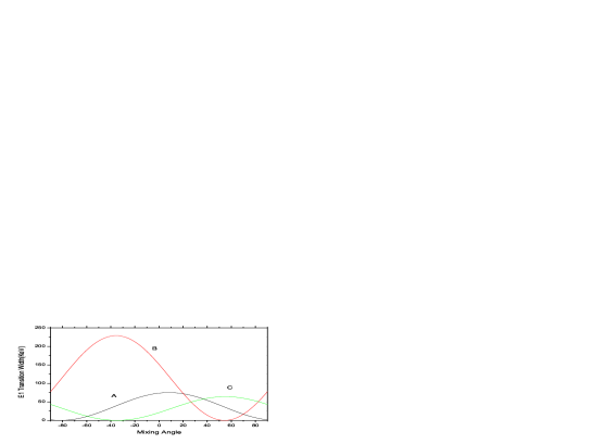
Figure 1: E1 transition widths of $\psi(4040)$ varying with 3S-2D mixing angle in Model I. A: $\psi(4040)\to\chi^{{}^{\prime}}_{c_{2}}(3929)\gamma$, B: $\psi(4040)\to\chi^{{}^{\prime}}_{c_{1}}(3872)\gamma$, C: $\psi(4040)\to\chi^{{}^{\prime}}_{c_{0}}(3915)\gamma$.

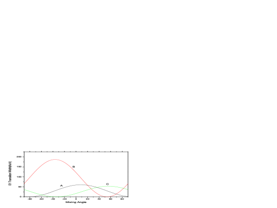
Figure 2: E1 transition widths of $\psi(4040)$ varying with 3S-2D mixing angle in Model II. A: $\psi(4040)\to\chi^{{}^{\prime}}_{c_{2}}(3929)\gamma$, B: $\psi(4040)\to\chi^{{}^{\prime}}_{c_{1}}(3872)\gamma$, C: $\psi(4040)\to\chi^{{}^{\prime}}_{c_{0}}(3915)\gamma$.

Figure 3: E1 transition widths of $\psi(4160)$ varying with 3S-2D mixing angle in Model I. A: $\psi(4160)\to\chi^{{}^{\prime}}_{c_{2}}(3929)\gamma$, B: $\psi(4160)\to\chi^{{}^{\prime}}_{c_{1}}(3872)\gamma$, C: $\psi(4160)\to\chi^{{}^{\prime}}_{c_{0}}(3915)\gamma$.

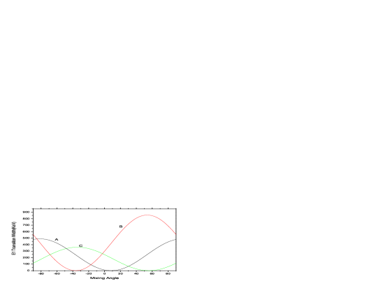
Figure 4: E1 transition widths of $\psi(4160)$ varying with 3S-2D mixing angle in Model II. A: $\psi(4160)\to\chi^{{}^{\prime}}_{c_{2}}(3929)\gamma$, B: $\psi(4160)\to\chi^{{}^{\prime}}_{c_{1}}(3872)\gamma$, C: $\psi(4160)\to\chi^{{}^{\prime}}_{c_{0}}(3915)\gamma$.

We see that the decay width of $\psi(4040)\to\chi^{{}^{\prime}}_{c_{2}}(3929)\gamma$ reaches its maximum of about 75 KeV corresponding to a branching ratio of $9.3\times 10^{-4}$ near $\theta=10^{o}$. While the decay width of $\psi(4160)\to\chi^{{}^{\prime}}_{c_{2}}(3929)\gamma$ reaches its minimum (zero) near $10^{o}$ and its maximum of about 600 KeV near $-80^{o}$ at which $\psi(4160)$ is almost a pure $\psi(3^{3}S_{1})$ and the corresponding branching ratio is about $6\times 10^{-3}$.

The decay width of $\psi(4040)\to\chi^{{}^{\prime}}_{c_{1}}(3872)\gamma$ reaches its maximum of about 250 KeV corresponding to a branching ratio of $3.1\times 10^{-3}$ near $-35^{o}$, which is about 2 times larger than that of non-mixing, and reaches its minimum (zero) near $55^{o}$. While the decay width of $\psi(4160)\to\chi^{{}^{\prime}}_{c_{1}}(3872)\gamma$ reaches its minimum (zero) near $-35^{o}$ and reaches its maximum of about 1050 KeV corresponding to a branching ratio of about 1% near $55^{o}$. It is very interesting to note that the two values happen to be corresponding to the mixing angles determined by leptonic decay widths of $\psi(4040)$ and $\psi(4160)$. That means, one of the two channels must be enhanced by the 3S-2D mixing if the mixing mechanism just affect the leptonic decays and the E1 transitions by simply mixing the wave functions.

The decay width of $\psi(4040)\to\chi^{{}^{\prime}}_{c_{0}}(3915)\gamma$ reaches its maximum of about 52 KeV corresponding to a branching ratio of $6.5\times 10^{-4}$ near $55^{o}$, which is about 2.5 times larger than that of non-mixing and reaches its minimum (zero) near $-35^{o}$. While the decay width of $\psi(4160)\to\chi^{{}^{\prime}}_{c_{0}}(3915)\gamma$ reaches its minimum (zero) near $55^{o}$ and reaches its maximum of about 450 KeV corresponding to a branching ratio of about $4.5\times 10^{-3}$ near $-35^{o}$.

Since the decay width of $\psi(4160)\to\chi^{{}^{\prime}}_{c_{2}}(3929)\gamma$ reaches its minimum (zero) and $\psi(4040)\to\chi^{{}^{\prime}}_{c_{2}}(3929)\gamma$ reaches its maximum near $10^{0}$, which is not far from the non-mixing case, in our model calculations, we may use these two channels to check whether there is substantial 3S-2D mixing between $\psi(4040)$ and $\psi(4160)$. If $\chi^{{}^{\prime}}_{c_{2}}(3929)$ can be detected in the E1 transitions from $\psi(4040)$ but not from $\psi(4160)$, then the mixing angle should be small. In general, since the Z(3930) is identified with $\chi^{{}^{\prime}}_{c_{2}}$, the observed E1 transition rates to Z(3930) from $\psi(4040)$ and $\psi(4160)$ will be useful to constrain the value of 3S-2D mixing angle by comparing the measurements and the theoretical predictions. When we have a better control over the value of mixing angle, we will be in a position to study the properties of X(3872) and X(3915), and to see if they can be respectively the $\chi^{{}^{\prime}}_{c_{1}}$ (or partially be) and $\chi^{{}^{\prime}}_{c_{0}}$ by comparing the observed E1 transition rates with theoretical predictions for $\psi(4040)$ and $\psi(4160)$ decays to $\chi^{{}^{\prime}}_{c_{1,0}}\gamma$. However, we must keep in mind that the 3S-2D mixing model for $\psi(4040)$ and $\psi(4160)$ is only a simplification for the real situation, since the mixing with 4S state and the charm meson pairs are all neglected in the 3S-2D mixing model. Nevertheless, with this simple model we hope some useful information can be obtained for these X,Y,Z states by measuring the E1 transition rates of $\psi(4040)$ and $\psi(4160)$ to $\chi^{{}^{\prime}}_{c_{J}}$ (J=2,1,0) charmonium states.

We also calculate the E1 transition widths of $\psi(4040,4160)\rightarrow\chi_{c_{J}}(1P)\gamma$ in order to see whether these can be helpful in determining the 3S-2D mixing angle. The results are listed in Table 3. Although the calculated widths are expectedly small, the transition branching ratio of $\chi_{c_{1,2}}\rightarrow J/\psi\,\gamma$ are relatively large (about 20% for $\chi_{c_{2}}$ and 36% for $\chi_{c_{1}}$). So hopefully it is possible to measure them in experiment if the data samples are large enough. A special case is $\psi(4160)\rightarrow\chi_{c_{1}}\gamma$ with a branching ratio of order $10^{-4}$, which is quite large, and might be easier to be detected. Again, if we have determined the mixing angle, it would help us searching for $\chi^{{}^{\prime}}_{c_{J}}$ and identify the X,Y,Z resonances.

Table 3: E1 transition widths and branching ratios of charmonium states in various potential models with lowest-order wave functions. The masses and total widths of the initial and final states used in the calculation are the PDG Nakamura:2010zzi central values.

Process		$<f|r|i>\,(GeV^{-1}$)			$\rm k\,(MeV)$			$\Gamma_{\rm thy}$ (keV)					$Br_{\rm thy}~{}(\times 10^{-4})$
Intial	Final	I	II	III	Ours	Ref.Barnes2005	Ref.Godfrey:1985xj	I	II	III	Ref.Barnes2005	Ref.Godfrey:1985xj	I	II	III	Ref.Barnes2005	Ref.Godfrey:1985xj
$\psi(4040)$	$\chi_{C2}(3556)$	0.026	0.078	-0.011	454	455	508	0.16	1.4	0.03	0.70	12.7	0.02	0.18	0.004	0.09	1.6
	$\chi_{C1}(3511)$	0.026	0.078	-0.011	493	494	547	0.12	1.1	0.02	0.53	0.85	0.02	0.14	0.003	0.07	0.11
	$\chi_{C0}(3415)$	0.026	0.078	-0.011	576	577	628	0.06	0.6	0.01	0.27	0.63	0.01	0.08	0.001	0.03	0.08
$\psi(4160)$	$\chi_{C2}(3556)$	0.43	0.34	0.23	554	559	590	1.5	0.9	0.4	0.79	0.027	0.15	0.09	0.04	0.08	0.003
	$\chi_{C1}(3511)$	0.43	0.34	0.23	592	598	628	28	17	7.9	14	3.4	2.7	1.7	0.77	1.4	0.33
	$\chi_{C0}(3415)$	0.43	0.34	0.23	672	677	707	55	33	15	27	35	5.3	3.2	1.5	2.6	3.4

V summary

In this paper, we calculate the E1 transition widths and branching ratios of $\psi(4040,4160,4415)\rightarrow\chi^{{}^{\prime}}_{c_{J}}\gamma$ in three typical potential models with both lowest- and first-order relativistically corrected wave functions. We find the transition widths of $\psi(4040,4160)\rightarrow\chi^{{}^{\prime}}_{c_{J}}$ are model-insensitive and relatively large (tens to hundreds of KeV) and the corresponding branching ratios are of order $10^{-4}-10^{-3}$, which make the search for $\chi^{{}^{\prime}}_{c_{J}}$ possible at $e^{+}e^{-}$ colliders such as BEPCII/BESIII and CESR/CLEO. This may help us identify some of the recently discovered X,Y,Z particles, especially the $X(3915)$, $Y(3915)$, $Y(3940)$ and $X(3872)$. The possible 3S-2D mixing of $\psi(4040)$ and $\psi(4160)$ and its effect on the transition widths of $\psi(4040,4160)\rightarrow\chi^{{}^{\prime}}_{c_{J}}\gamma$ are considered and found to be important. We find the transitions $\psi(4040,4160)\rightarrow\chi^{{}^{\prime}}_{c_{2}}\gamma$ can be used to examine whether the mixing exists and to further possibly constrain the mixing angle; and the transitions $\psi(4040,4160)\rightarrow\chi^{{}^{\prime}}_{c_{1}}\gamma$ and $\psi(4040,4160)\rightarrow\chi^{{}^{\prime}}_{c_{0}}\gamma$ can be used to estimate how far is the mixing angle from $-35^{o}$ and $55^{o}$, which are determined in a simple 3S-2D mixing model by the observed leptonic decay widths of $\psi(4040)$ and $\psi(4160)$. The transitions of $\psi(4040,4160)\rightarrow\chi_{c_{J}}(1P)\gamma$ are also discussed, and the $\psi(4160)\rightarrow\chi_{c_{1}}\gamma$ transition is found to have a branching ratio of order of $10^{-4}$, which may be relatively easier to be detected.

VI acknowledgement

We would like to thank Chang-Zheng Yuan for many valuable discussions. This work was supported in part by the National Natural Science Foundation of China (No 11047156, No 11075002, No 11021092, No 10905001), and the Ministry of Science and Technology of China (2009CB825200).

References

- (1) J. J. Aubert et al. [E598 Collaboration], Phys. Rev. Lett. 33, 1404 (1974).
- (2) J. E. Augustin et al. [SLAC-SP-017 Collaboration], Phys. Rev. Lett. 33, 1406 (1974).
- (3) D.M. Asner et al., Int.J.Mod.Phys. A24 (2009) S1-794 [arXiv:0809.1869 [hep-ex]].
- (4) B. Q. Li, C. Meng and K. T. Chao, Phys. Rev. D 80, 014012 (2009) [arXiv:0904.4068 [hep-ph]].
- (5) N. Brambilla et al., Eur. Phys. J. C71, 1534 (2011). [arXiv:1010.5827 [hep-ph]].
- (6) E. Eichten, K. Gottfried, T. Kinoshita, K.D. Lane and T. M. Yan, Phys. Rev. D 17, 3090 (1978) [Erratum-ibid. 21, 313 (1980)]; 21, 203 (1980).
- (7) T. Barnes, S. Godfrey and E.S. Swanson, Phys. Rev. D 72, 054026 (2005).
- (8) S. Godfrey and N. Isgur, Phys. Rev. D 32, 189 (1985).
- (9) S. Uehara et. al. [Belle Collaboration], Phys. Rev. Lett. 96, 082003 (2006).
- (10) S. Uehara et al. [Belle Collaboration], Phys. Rev. Lett. 104, 092001 (2010) [arXiv:0912.4451 [hep-ex]].
- (11) X. Liu, Z. G. Luo and Z. F. Sun, Phys. Rev. Lett. 104, 122001 (2010) [arXiv:0911.3694 [hep-ph]].
- (12) K. Abe et al. [Belle Collaboration], Phys. Rev. Lett. 94, 182002 (2005) [arXiv:hep-ex/0408126].
- (13) B. Aubert et al. [BaBar Collaboration], Phys. Rev. Lett. 101, 082001 (2008) [arXiv:0711.2047 [hep-ex]].
- (14) K. Abe et. al. [Belle Collaboration], Phys. Rev. Lett. 98, 082001 (2007).
- (15) B. Q. Li and K. T. Chao, Phys. Rev. D 79, 094004 (2009) [arXiv:0903.5506 [hep-ph]].
- (16) G. Pakhlova et al. [Belle Collaboration], Phy. Rev. Lett. 100, 202001 (2008).
- (17) S. K. Choi et al. [Belle Collaboration], Phys. Rev. Lett. 91, 262001 (2003) [arXiv:hep-ex/0309032].
- (18) Y. B. Ding, J. He, S. O. Cai, D. H. Qin and K. T. Chao, IN *PEKING 1985, PROCEEDINGS, PARTICLE AND NUCLEAR PHYSICS* 88-91.
- (19) Y. B. Ding, D. H. Qin and K. T. Chao, Phys. Rev. D 44, 3562 (1991).
- (20) W. Lucha, F. F. Schoberl and D. Gromes, Phys. Rept. 200, 127 (1991).
- (21) W. Kwong and J. L. Rosner, Phys. Rev. D 38, 279 (1988).
- (22) K. Nakamura et al. [ Particle Data Group Collaboration ], J. Phys. G G37, 075021 (2010).
- (23) and B. Aubert [The BABAR Collaboration], Phys. Rev. D 81, 092003 (2010) [arXiv:1002.0281 [hep-ex]].
- (24) C. Z. Yuan [Belle Collaboration], arXiv:0910.3138 [hep-ex].
- (25) A. Zupanc [Belle Collaboration], arXiv:0910.3404 [hep-ex].
- (26) S. Godfrey, arXiv:0910.3409 [hep-ph].
- (27) T. Branz, T. Gutsche and V. E. Lyubovitskij, Phys. Rev. D 80, 054019 (2009) [arXiv:0903.5424 [hep-ph]].
- (28) X. Liu and S. L. Zhu, Phys. Rev. D 80, 017502 (2009) [arXiv:0903.2529 [hep-ph]].
- (29) J. R. Zhang and M. Q. Huang, Phys. Rev. D 80, 056004 (2009) [arXiv:0906.0090 [hep-ph
- (30) T. Aushev et al., Phys. Rev. D 81, 031103 (2010).
- (31) see the website: http://www-cdf.fnal.gov/physics/new/ bottom/080724.blessed-X-Mass.
- (32) C. Cawlfield et al. [CLEO Collaboration], Phys. Rev. Lett. 98 092002 (2007).
- (33) K. Abe et al. [Belle Collaboration], arXiv: hep-ex/0505038.
- (34) A. Aulencia et al. [CDF Collaboration], Phy. Rev. Lett. 96, 102002 (2006), 98, 132002 (2007).
- (35) T. Barnes and S. Godfrey, Phys. Rev. D 69, 054008 (2004) [arXiv:hep-ph/0311162].
- (36) E. J. Eichten, K. Lane and C. Quigg, Phys. Rev. D 69, 094019 (2004) [arXiv:hep-ph/0401210].
- (37) C. Meng, Y. J. Gao and K. T. Chao, arXiv:hep-ph/0506222.
- (38) M. Suzuki, Phys. Rev. D 72, 114013 (2005) [arXiv:hep-ph/0508258].
- (39) P. del Amo Sanchez et al. [ BABAR Collaboration ], Phys. Rev. D82, 011101 (2010). [arXiv:1005.5190].
- (40) Y. Jia, W. -L. Sang, J. Xu, [arXiv:1007.4541].
- (41) T. J. Burns, F. Piccinini, A. D. Polosa, C. Sabelli, Phys. Rev. D82, 074003 (2010). [arXiv:1008.0018].
- (42) Y. S. Kalashnikova, A. V. Nefediev, Phys. Rev. D82, 097502 (2010) [arXiv:1008.2895].
- (43) Y. Fan, J. Z. Li, C. Meng, K. T. Chao, arXiv:1112.3625.
- (44) F. E. Close and P. R. Page, Phys. Lett. B 366, 323 (1996) [arXiv:hep-ph/9507407].
- (45) K.T.Chao, Phys.Lett. B661,348(2008) [arXiv:0707.3982].
- (46) A.M. Badalian, B.L.G. Bakker, and I.V. Danilkin, Phys. Atom. Nucl. 72, 638 (2009) [arXiv:0805.2291].