Counting spanning trees in a small-world Farey graph

Abstract

The problem of spanning trees is closely related to various interesting problems in the area of statistical physics, but determining the number of spanning trees in general networks is computationally intractable. In this paper, we perform a study on the enumeration of spanning trees in a specific small-world network with an exponential distribution of vertex degrees, which is called a Farey graph since it is associated with the famous Farey sequence. According to the particular network structure, we provide some recursive relations governing the Laplacian characteristic polynomials of a Farey graph and its subgraphs. Then, making use of these relations obtained here, we derive the exact number of spanning trees in the Farey graph, as well as an approximate numerical solution for the asymptotic growth constant characterizing the network. Finally, we compare our results with those of different types of networks previously investigated.

1 Introduction

Counting spanning trees in networks (graphs) is a fascinating and central issue in statistical physics, because of its inherent relevance to diverse aspects in related fields. For example, the number of spanning trees is an important measure of reliability of a network [1, 2]. Again for instance, it is exactly the number of recurrent configurations of the Abelian sand-pile models [3, 5, 4], which have been studied extensively in the past two decades as a paradigm of the self-organized criticality [6, 7]. On the other hand, the problem of spanning trees has numerous connections with other interesting problems associated with networks, such as dimer coverings [8], Potts model [4, 9], random walks [10, 11], origin of fractalitity for fractal scale-free networks [12, 13] and many others [14].

In view of its wide range of applications, the enumeration of spanning trees has received considerable attentions from the scientific community. A lot of previous studies have focused on counting spanning trees on different media, including regular lattices [15, 16, 17], the Sierpinski gaskets [18], and the Erdös-Rényi random graphs [19], even scale-free networks [20, 21] that display the striking power-law degree distribution [22] as found for many real systems [23, 24, 25, 26]. These researches uncovered the impacts of various architectures on the number of spanning trees in different networks. However, not all real-word networks are scale-free. It has been observed [27] that the degree distribution of some real-life networks (e.g., power grid) decays exponentially, although they show small-world effect [28] characterized simultaneously by low average path length and high clustering coefficient. Thus far, the problem of spanning trees in small-world networks with an exponential degree distribution has not been addressed.

In this paper, we count spanning trees in a small-world network with a connectivity distribution decaying exponentially, which is translated from the Farey sequence [29] and thus called a Farey graph (network). According to the specific structure of the Farey graph, we derive recurrence formulas for the Laplacian characteristic polynomials of Farey graph and its subgraphs, based on which we determine the exact number of spanning trees in Farey graph and numerical value of its asymptotic growth constant. We also compare our results with those for other networks with the same average degree of nodes but different degree distributions.

2 Construction and topological properties of Farey graph

The graph under consideration is derived from the famous Farey sequence [29]. In mathematics, a Farey sequence of order $n$ ($n$ is a positive integer) is a set (denoted by $F_{n}$) of irreducible fractions between 0 and 1 arranged in an increasing order, the denominators of which do not exceed $n$. For example, the first four Farey sequences are: $F_{1}=\{{0\over 1},{1\over 1}\}$, $F_{2}=\{{0\over 1},{1\over 2},{1\over 1}\}$, $F_{3}=\{{0\over 1},{1\over 3},{1\over 2},{2\over 3},{1\over 1}\}$, $F_{4}=\{{0\over 1},{1\over 4},{1\over 3},{1\over 2},{2\over 3},{3\over 4},{1\over 1}\}$. In fact, Farey sequence $F_{n}$ can be constructed from $F_{n-1}$ by using the Farey sum operation denoted as $\oplus$. Let $a\over b$ and $c\over d$ be two irreducible fractions, then one can define their “mediant” as $\frac{a}{b}\oplus\frac{c}{d}={{a+c}\over{b+d}}$. It has been proved that $F_{n}$ could be obtained from $F_{n-1}$ by calculating the mediant between each pair of consecutive fractions in $F_{n-1}$, keeping only those mediants with denominator equal to $n$, and placing each mediant between the two values from which it was derived. The Farey sequence has an interesting property, that is say, any two neighboring fractions $p\over q$ and $r\over s$ in a Farey sequence satisfy $rq-ps=1$.

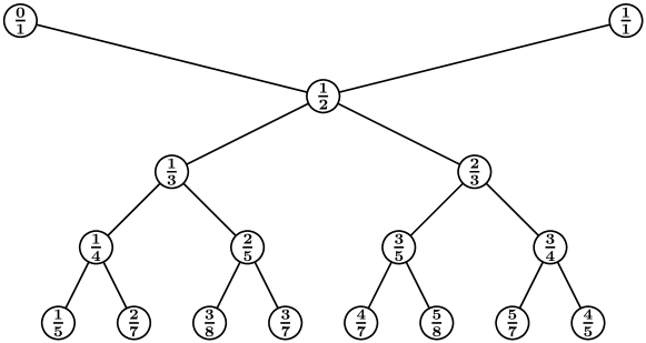
Figure 1: Illustration of a Farey tree for the first several levels.

The Farey sequence can be organized in the so-called Farey tree [30, 31]. Beginning with the two fractions $0\over 1$ and $1\over 1$, the first level of the tree is ${1\over 2}={0\over 1}\oplus{1\over 1}$, and the second level consists of two fractions $1\over 3$ and $2\over 3$ that are obtained by the Farey sum operation over all the previous fractions, i.e., ${1\over 3}={0\over 1}\oplus{1\over 2}$ and ${2\over 3}={1\over 2}\oplus{1\over 1}$. Repeating this Farey addition recursively, we can obtain the Farey tree, the $n$th level of which includes $2^{n-1}$ irreducible fractions, see Fig 1. In addition, based on the Farey tree, one can construct a small-world graph called Farey graph [32, 33], in which nodes represent the irreducible fractions between 0 and 1, and two nodes $p\over q$ and $r\over s$ are connected if they satisfy the relation $rq-ps=1$, or equivalently if they are consecutive terms in some Farey sequence, see Fig 2. Notice that, the Farey tree is actually a spanning tree of the Farey graph.

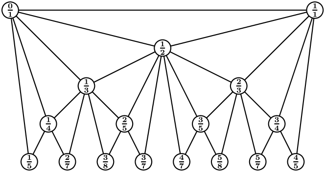
Figure 2: Illustration of a Farey graph corresponding to the Farey tree depicted in Fig. 1.

In fact, the Farey graph can be created in the following iterative way [34, 35]. Let $W_{g}$ denote the Farey graph after $g$ iterations. For $g=0$, $W_{g}$ is an edge connecting two nodes. For $g\geq 1$, $W_{g}$ is obtained from $W_{g-1}$: for each edge in $W_{g-1}$ introduced at iteration $g-1$, we add a new node and attach it to both ends of the edge. The Farey graph is minimally 3-colorable, uniquely Hamiltonian, and maximally outerplanar [32, 36]. Particularly, the Farey graph exhibits some remarkable properties of real networks, it is small world with its average distance increasing logarithmically with its node number, and its clustering coefficient converges to a large constant $\ln 2$ [34, 35].

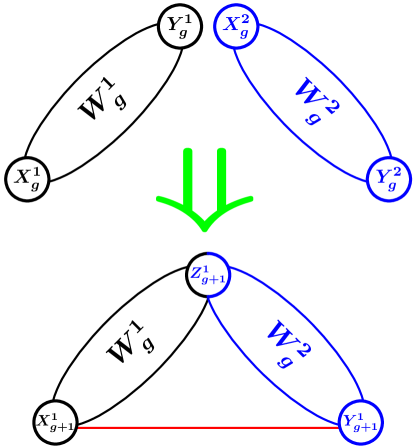
Figure 3: (Color online) Alternative construction method of the Farey graph. $W_{g+1}$ can be obtained by joining two copies of $W_{g}$ denoted as $W_{g}^{\eta}$ ($\eta=1,2$), the initial nodes of which are represented by $X_{g}^{\eta}$ and $Y_{g}^{\eta}$, respectively. In the merging process, $Y_{g}^{1}$ and $X_{g}^{2}$ are identified as the hub node $Z_{g+1}$ of $W_{g+1}$. In addition, $X_{g}^{1}$ and $Y_{g}^{2}$ become respectively $X_{g+1}$ and $Y_{g+1}$, which are linked to each other by a new edge.

3 Spanning trees on Farey graph

After introducing the network construction and its structural properties, we continue to investigate spanning trees in the Farey graph $W_{g}$, by establishing and using recursive relations for the characteristic polynomials of it and its subgraphs at different iterations. To facilitate the description, we give the following definitions. Let $X_{g}$ and $Y_{g}$ denote the two nodes in graph $W_{g}$ that are created at iteration 0 and thus called initial nodes. In addition, the node in $W_{g}$ having the highest degree was generated at iteration 1, it is thus named the hub node and represented by $Z_{g}$. Then, the Farey graph can be alternatively built as follows. Given iteration $g$, $W_{g+1}$ may be obtained by joining at the initial nodes two copies of $W_{g}$, see Fig. 3. This new construction shows that the Farey graph is self-similar, implying that the network order (represented by $N_{g}$) obeys $N_{g}=2N_{g-1}-1$, which coupled with $N_{0}=2$ gives $N_{g}=2^{g}+1$. Using the self-similar property of the Farey graph, one can enumerate the number of spanning trees, which is the focus of this paper.

According to the well-known matrix-tree theorem [37], the number of spanning trees in a connected graph can be expressed numerically but exactly in terms of the Laplacian spectra corresponding to the graph. Let $N_{\rm ST}(g)$ represent the number of spanning trees in the Farey network $W_{g}$, whose Laplacian matrix is represented by $\textbf{L}_{g}=[L_{ij}]$, then one can obtain $N_{\rm ST}(g)$ by computing the product of all non-zero eigenvalues of $\textbf{L}_{g}$ as [38, 39]

$$N_{\rm ST}(g)=\frac{1}{N_{g}}\prod_{i=1}^{N_{g}-1}\lambda_{i}(g)\,,$$ (1)

where $\lambda_{i}(g)$ ($i=1,2,\ldots,N_{g}-1$) denote the $N_{g}-1$ non-zero eigenvalues of matrix $\textbf{L}_{g}$, the entry $L_{ij}$ of which is defined as follows: $L_{ij}=-1$ (or $0$) if nodes $i$ and $j$ are (or not) adjacent and $i\neq j$, $L_{ij}$ equals the degree of node $i$ if $i=j$.

Equation (1) shows that the issue of determining $N_{\rm ST}(g)$ is reduced to finding the product of all nonzero Laplacian eigenvalues. Although the expression of Eq. (1) appears succinct, it requires computing the eigenvalues of a matrix with order $N_{g}\times N_{g}$, which make heavy demands on time and computational resources for large networks, since the complexity for calculating eigenvalues is very high. Thus, for large networks, it is not acceptable to obtain $N_{\rm ST}(g)$ through direct calculation of the Laplacian spectra, due to the limitations of time and computer memory. It is then of significant practical importance to seek for a computationally cheaper approach to overcome this problem. Fortunately, the self-similar architecture of the Farey graph allows for calculating the product of its nonzero Laplacian eigenvalues to obtain an analytical solution to the number of spanning trees. Details will be provided below.

We use $P_{g}(\lambda)$ to denote the characteristic polynomial of the Laplacian matrix ${\bf L}_{g}$, i.e.,

$$P_{g}(\lambda)={\rm det}({\bf L}_{g}-\lambda{\bf I}_{g})\,,$$ (2)

in which ${\bf I}_{g}$ is an $N_{g}\times N_{g}$ identity matrix. As mentioned above, our goal is to evaluate the product of all the nonzero eigenvalues of ${\bf L}_{g}$, namely, all nonzero roots of polynomial $P_{g}(\lambda)$.

In order to find the product, we denote ${\bf Q}_{g}$ as an $(N_{g}-1)\times(N_{g}-1)$ submatrix of $({\bf L}_{g}-\lambda{\bf I}_{g})$, which is obtained by removing from $({\bf L}_{g}-\lambda{\bf I}_{g})$ the row and column corresponding to an initial node, say, node $X_{g}$ of network $W_{g}$. In addition, we use ${\bf R}_{g}$ to represent a submatrix of $({\bf L}_{g}-\lambda{\bf I}_{g})$ with an order $(N_{g}-2)\times(N_{g}-2)$, obtained from $({\bf L}_{g}-\lambda{\bf I}_{g})$ by removing from it the two rows and columns corresponding to the two initial nodes in $W_{g}$, i.e., $X_{g}$ and $Y_{g}$. On the other hand, let $Q_{g}(\lambda)$ and $R_{g}(\lambda)$ denote respectively the determinants of ${\bf Q}_{g}$ and ${\bf R}_{g}$. Then, the three quantities $P_{g}(\lambda)$, $Q_{g}(\lambda)$, and $R_{g}(\lambda)$ obey the following relations:

$$P_{g+1}(\lambda)=\left|\begin{array}[]{ccc}2d_{g}-\lambda&l_{q}&l_{q}\\ l_{q}^{\top}&{\bf Q}_{g}+{\bf E}_{g}&-{\bf E}_{g}\\ l_{q}^{\top}&-{\bf E}_{g}&{\bf Q}_{g}+{\bf E}_{g}\end{array}\right|,$$ (3)

$$Q_{g+1}(\lambda)=\left|\begin{array}[]{ccc}2d_{g}-\lambda&l_{q}&l_{r}\\ l_{q}^{\top}&{\bf Q}_{g}+{\bf E}_{g}&{\bf O}\\ l_{r}^{\top}&{\bf O}&{\bf R}_{g}\end{array}\right|,$$ (4)

and

$$R_{g+1}(\lambda)=\left|\begin{array}[]{ccc}2d_{g}-\lambda&l_{r}&l_{r}\\ l_{r}^{\top}&{\bf R}_{g}&{\bf O}\\ l_{r}^{\top}&{\bf O}&{\bf R}_{g}\end{array}\right|\,.$$ (5)

In Eqs. (3-5), ${\bf E}_{g}$ is an $(N_{g}-1)\times(N_{g}-1)$ square matrix with only one entry equal to 1 while all other entries being 0, viz.,

$${\bf E}_{g}=\left(\begin{array}[]{cccc}1&0&\cdots&0\\ 0&0&\cdots&0\\ \vdots&\vdots&&\vdots\\ 0&0&\cdots&0\end{array}\right)\,;$$ (10)

$2d_{g}$ expresses the degree of the hub node $Z_{g+1}$ in the $(g+1)$th generation $W_{g+1}$, which is in fact the double of the degree, $d_{g}$, of an initial node $X_{g}$ or $Y_{g}$ in graph $W_{g}$; $l_{q}$ ($l_{r}$) is a vector of order $N_{g}-1$ ($N_{g}-2$) with $d_{g}$ entries being $-1$ all other $N_{g}-d_{g}-1$ ($N_{g}-d_{g}-2$) entries equaling 0, in which each entry $-1$ describes an edge connecting the hub node $Z_{g+1}$ and a node belonging to either $W_{g}^{1}$ or $W_{g}^{2}$, both of which are amalgamated into $W_{g+1}$; finally, the superscript $\top$ of a vector represents transpose.

For the convenience of following description, we index respectively the rows and columns of $P_{g+1}(\lambda)$ (or its variants obtained from it by elementary matrix operations) by $V_{i}$ and $C_{i}$ with $i=1,2,\ldots,2N_{g}-1$. Applying the elementary matrix operation, i.e., replacing column $C_{j}(N_{g}+1\leq j\leq 2N_{g}-1)$ by $C_{j}-C_{j-N_{g}+1}$, we have

$$P_{g+1}(\lambda)=\left|\begin{array}[]{ccc}2d_{g}-\lambda&l_{q}&{\bf 0}\\ l_{q}^{\top}&{\bf Q}_{g}+{\bf E}_{g}&-({\bf Q}_{g}+2{\bf E}_{g})\\ l_{q}^{\top}&-{\bf E}_{g}&{\bf Q}_{g}+2{\bf E}_{g}\end{array}\right|.$$ (14)

We continue to replace the row $V_{i}(2\leq i\leq N_{g})$ in Eq. (14) by $V_{i}+V_{i+N_{g}-1}$, yielding

$$P_{g+1}(\lambda) = \left|\begin{array}[]{ccc}2d_{g}-\lambda&l_{q}&{\bf 0}\\ 2l_{q}^{\top}&{\bf Q}_{g}&{\bf O}\\ l_{q}^{\top}&-{\bf E}_{g}&{\bf Q}_{g}+2{\bf E}_{g}\end{array}\right|$$ (18)

$$= \left|\begin{array}[]{cc}2d_{g}-\lambda&l_{q}\\ 2l_{q}^{\top}&{\bf Q}_{g}\end{array}\right|\left|{\bf Q}_{g}+2{\bf E}_{g}\right|.$$ (21)

Thus, we have expressed the $P_{g+1}(\lambda)$ as a product of two determinants, which we denote by $P_{g+1}^{(1)}(\lambda)$ and $P_{g+1}^{(2)}(\lambda)$, respectively. These two determinants can be easily evaluated as

$$P_{g+1}^{(1)}(\lambda) = \left|\begin{array}[]{cc}2d_{g}-2\lambda&l_{q}\\ 2l_{q}^{\top}&{\bf Q}_{g}\end{array}\right|+\left|\begin{array}[]{cc}\lambda&{\bf 0}\\ 2l_{q}^{\top}&{\bf Q}_{g}\end{array}\right|$$ (26)

$$= 2P_{g}(\lambda)+\lambda Q_{g}(\lambda)$$ (27)

and

$$P_{g+1}^{(2)}(\lambda) = \left|{\bf Q}_{g}\right|+2\left|{\bf R}_{g}\right|=Q_{g}(\lambda)+2R_{g}(\lambda).$$ (28)

Inserting Eqs. (26) and (28) into Eq. (18), we have

$$P_{g+1}(\lambda) = [2P_{g}(\lambda)+\lambda Q_{g}(\lambda)][Q_{g}(\lambda)+2R_{g}(\lambda)]$$ (29)

$$= 2P_{g}(\lambda)Q_{g}(\lambda)+4P_{g}(\lambda)R_{g}(\lambda)$$

$$+\lambda[(Q_{g}(\lambda))^{2}+2Q_{g}(\lambda)R_{g}(\lambda)]\,.$$

Similar to the computation processes for $P_{g+1}^{(1)}(\lambda)$ and $P_{g+1}^{(2)}(\lambda)$, $Q_{g+1}(\lambda)$ and $R_{g+1}(\lambda)$ can be calculated as shown in Eqs. (36) and (51).

$$Q_{g+1}(\lambda) = \left|\begin{array}[]{ccc}d_{g}-\lambda&l_{q}&{\bf 0}\\ l_{q}^{\top}&{\bf Q}_{g}+{\bf E}_{g}&{\bf O}\\ l_{r}^{\top}&{\bf O}&{\bf R}_{g}\end{array}\right|+\left|\begin{array}[]{ccc}d_{g}-\lambda&{\bf 0}&l_{r}\\ l_{q}^{\top}&{\bf Q}_{g}+{\bf E}_{g}&{\bf O}\\ l_{r}^{\top}&{\bf O}&{\bf R}_{g}\end{array}\right|$$ (36)

$$+\left|\begin{array}[]{ccc}\lambda&{\bf 0}&{\bf 0}\\ l_{q}^{\top}&{\bf Q}_{g}+{\bf E}_{g}&{\bf O}\\ l_{r}^{\top}&{\bf O}&{\bf R}_{g}\end{array}\right|$$

$$= R_{g}(\lambda)[P_{g}(\lambda)+Q_{g}(\lambda)]+Q_{g}(\lambda)[Q_{g}(\lambda)+R_{g}(\lambda)]$$

$$+\lambda R_{g}(\lambda)[Q_{g}(\lambda)+R_{g}(\lambda)],$$ (41)

$$R_{g+1}(\lambda) = \left|\begin{array}[]{ccc}d_{g}-\lambda&l_{r}&{\bf 0}\\ l_{r}^{\top}&{\bf R}_{g}&{\bf O}\\ l_{r}^{\top}&{\bf O}&{\bf R}_{g}\end{array}\right|+\left|\begin{array}[]{ccc}d_{g}-\lambda&{\bf 0}&l_{r}\\ l_{r}^{\top}&{\bf R}_{g}&{\bf O}\\ l_{r}^{\top}&{\bf O}&{\bf R}_{g}\end{array}\right|+\left|\begin{array}[]{ccc}\lambda&{\bf 0}&{\bf 0}\\ l_{r}^{\top}&{\bf R}_{g}&{\bf O}\\ l_{r}^{\top}&{\bf O}&{\bf R}_{g}\end{array}\right|$$ (51)

$$= Q_{g}(\lambda)R_{g}(\lambda)+Q_{g}(\lambda)R_{g}(\lambda)+\lambda[R_{g}(\lambda)]^{2}.$$ (52)

Having derived the recursive relations for $P_{g}(\lambda)$, $Q_{g}(\lambda)$, and $R_{g}(\lambda)$, shown in Eqs. (29-51), we proceed to compute the product of the nonzero roots of polynomial $P_{g}(\lambda)$. Since $P_{g}(\lambda)$ has one and only one root equal to zero, say $\lambda_{0}(g)=0$, to find this product, we define a new polynomial $\bar{P}_{g}(\lambda)$ as

$$\bar{P}_{g}(\lambda)=\frac{1}{\lambda}P_{g}(\lambda)\,.$$ (53)

Then, it is evident that

$$\prod_{i=1}^{N_{g}-1}\lambda_{i}(g)=\prod_{i=1}^{N_{g}-1}\bar{\lambda}_{i}(g)\,,$$ (54)

in which $\bar{\lambda}_{1}(g),\bar{\lambda}_{2}(g),\ldots,\bar{\lambda}_{N_{g}-1}(g)$ represent the $N_{g}-1$ roots of polynomial $\bar{P}_{g}(\lambda)$. Thus, the determination of the product of nonzero eigenvalues of Laplacian matrix ${\bf L}_{g}$ is equivalent to calculating the product on the right-hand side (rhs) of Eq. (54).

To find the product $\prod_{i=1}^{N_{g}-1}\bar{\lambda}_{i}(g)$, we express polynomial $\bar{P}_{g}(\lambda)$ in the following form, i.e., $\bar{P}_{g}(\lambda)=\sum_{j=0}^{N_{g}-1}\bar{p}_{g}(j)\lambda^{j}$, in which $\bar{p}_{g}(j)$ is the coefficient of term $\lambda^{j}$ with degree $j$. Since it is obvious that $\bar{p}_{g}(N_{g}-1)=-1$, we then have

$$\sum_{j=0}^{N_{g}-1}\bar{p}_{g}(j)\lambda^{j}=-\prod_{i=1}^{N_{g}-1}[\lambda-\bar{\lambda}_{i}(g)]\,.$$ (55)

According to Vieta’s formulas, the following relation holds:

$$\prod_{i=1}^{N_{g}-1}\bar{\lambda}_{i}(g)=-\bar{p}_{g}(0)\,.$$ (56)

Thus, all we need is to determine the constant term $\bar{p}_{g}(0)$ of polynomial $\bar{P}_{g}(\lambda)$.

From Eqs. (29-51) it is not difficult to derive the following recursion equations:

$$\bar{P}_{g+1}(\lambda)=2\bar{P}_{g}(\lambda)Q_{g}(\lambda)+4\bar{P}_{g}(\lambda)R_{g}(\lambda)$$

$$+[Q_{g}(\lambda)]^{2}+2Q_{g}(\lambda)R_{g}(\lambda),$$ (57)

$$Q_{g+1}(\lambda) = [Q_{g}(\lambda)]^{2}+2Q_{g}(\lambda)R_{g}(\lambda)+\lambda[\bar{P}_{g}(\lambda)R_{g}(\lambda)$$ (58)

$$+Q_{g}(\lambda)R_{g}(\lambda)+(R_{g}(\lambda))^{2}],$$

and

$$R_{g+1}(\lambda)=2Q_{g}(\lambda)R_{g}(\lambda)+\lambda[R_{g}(\lambda)]^{2}.$$ (59)

On the basis of above relations, we can find the value for $\bar{p}_{g}(0)$. To this end, we give some additional variables. Let $q_{g}(0)$ and $r_{g}(0)$ be the constant terms of $Q_{g}(\lambda)$ and $R_{g}(\lambda)$, respectively. According to Eqs. (3-59), the three quantities $\bar{p}_{g}(0)$, $q_{g}(0)$ and $r_{g}(0)$ obey the recursive relations:

$$\bar{p}_{g+1}(0)=2\bar{p}_{g}(0)q_{g}(0)+4\bar{p}_{g}(0)r_{g}(0)+[q_{g}(0)]^{2}+2q_{g}(0)r_{g}(0)\,,$$ (60)

$$q_{g+1}(0)=[q_{g}(0)]^{2}+2q_{g}(0)r_{g}(0)\,,$$ (61)

and

$$r_{g+1}(0)=2q_{g}(0)r_{g}(0)\,.$$ (62)

Plugging Eq. (62) into Eq. (61) to obtain

$$q_{g+1}(0)=[q_{g}(0)]^{2}+r_{g+1}(0)\,,$$ (63)

which can be rephrased as

$$r_{g+1}(0)=q_{g+1}(0)-[q_{g}(0)]^{2}\,.$$ (64)

Replacing $r_{g}(0)$ in Eq. (62) by the expression given on the rhs of Eq. (64) leads to

$$q_{g+1}(0)=3[q_{g}(0)]^{2}-2q_{g}(0)[q_{g-1}(0)]^{2}.$$ (65)

Thus, we obtain the recursive relation governing $q_{g+1}(0)$, $q_{g}(0)$, and $q_{g-1}(0)$, as shown explicitly in Eq. (65).

Solving Eq. (65) one can arrive at the formula for $q_{g}(0)$. For this purpose, we introduce an intermediary quantity $k_{g}$, defined as

$$k_{g}=q_{g}(0)/[q_{g-1}(0)]^{2}\,,$$ (66)

making use of which Eq. (65) can be rewritten as

$$k_{g+1}=3-\frac{2}{k_{g}}\,.$$ (67)

Considering the initial condition $k_{1}=q_{1}(0)/[q_{0}(0)]^{2}=3$, Eq. (67) can be solved to yield

$$k_{g}=\frac{2(-1)^{g}-(-2)^{-g}}{(-1)^{g}-(-2)^{-g}}\,.$$ (68)

With the obtained exact result for $k_{g}$, we can reword Eq. (66) as

$$\ln{q_{g}(0)}=2\ln{q_{g-1}(0)}+\ln{k_{g}}\,.$$ (69)

Using the initial condition $\ln{q_{1}(0)}=\ln{3}$ and the expression for $k_{g}$ provided by Eq. (68), Eq. (69) can be solved inductively to obtain

$$\ln{q_{g}(0)}=2^{g-1}\sum_{i=0}^{g-1}2^{-i}\ln{\frac{2^{i+2}-1}{2^{i+1}-1}}\,.$$ (70)

Thus, we have

$$q_{g}(0) = \prod_{i=0}^{g-1}\left(\frac{2^{i+2}-1}{2^{i+1}-1}\right)^{2^{g-i-1}}$$ (71)

$$= \left(2^{g+1}-1\right)\prod_{i=2}^{g}\left(2^{i}-1\right)^{2^{g-i}}\,.$$

After deriving $q_{g}(0)$, we now are in position to calculate $\bar{p}_{g}(0)$. Notice that Eq. (60) can be decomposed into a product of two terms as

$$\bar{p}_{g+1}(0)=[2\bar{p}_{g}(0)+q_{g}(0)][q_{g}(0)+2r_{g}(0)]\,.$$ (72)

In addition, Eq. (61) can be rewritten as

$$q_{g+1}(0)=q_{g}(0)[q_{g}(0)+2r_{g}(0)]\,.$$ (73)

Then, we have

$$\frac{\bar{p}_{g+1}(0)}{q_{g+1}(0)}=2\frac{\bar{p}_{g}(0)}{q_{g}(0)}+1\,,$$ (74)

which together with $\bar{p}_{1}(0)/q_{1}(0)=-3$ leads to

$$\frac{\bar{p}_{g}(0)}{q_{g}(0)}=-\left(2^{g}+1\right)\,.$$ (75)

Thus, we can obtain the explicit formula for $\bar{p}_{g}(0)$:

$$\bar{p}_{g}(0)=-\left(2^{g}+1\right)\left(2^{g+1}-1\right)\prod_{i=2}^{g}\left(2^{i}-1\right)^{2^{g-i}}\,.$$ (76)

Hence, the number of spanning trees in the Farey graph $W_{g}$ is:

$$N_{\rm ST}(g)=-\frac{\bar{p}_{g}(0)}{N_{g}}=\left(2^{g+1}-1\right)\prod_{i=2}^{g}\left(2^{i}-1\right)^{2^{g-i}}\,.$$ (77)

Equation (77) is our main result, which is exact and holds for any legal $g$. Note that Eq. (77) can also be derived using another approach provided in the appendix. We thank an anonymous referee reminding us of this nice method.

Using the above-obtained result given by Eq. (77), one can determine the asymptotic growth constant of the spanning trees—an important quantity characterizing network structure— for the Farey graph, which is defined as the limiting value [40, 41]

$$E_{W_{g}}=\lim_{N_{g}\rightarrow\infty}\frac{\ln N_{\rm ST}(g)}{N_{g}}=\lim_{g\rightarrow\infty}\frac{\ln N_{\rm ST}(g)}{N_{g}}\,$$ (78)

that converges to a constant value $0.9458$, a finite number a little smaller than 1.

The obtained entropy of spanning trees for $W_{g}$ can be compared to those previously found for other media with the same average node degree as the Farey network. In the pseudofractal fractal web, the entropy is $0.8959$ [20], a value less than $0.9458$. For the square lattice and the two-dimensional Sierpinski gasket, their entropy of spanning trees are $1.16624$ [15] and $1.0486$ [18], respectively, both of which are greater than $0.9458$. Therefore, the number of spanning trees in the Farey graph is larger than that of the pseudofractal fractal web, but is smaller than that corresponding to the square lattice or the two-dimensional Sierpinski gasket. The distinctness lies with the architecture of these networks. Although they have identical average node degree, they show quite different degree distributions. Thus they exhibit disparate distribution of Laplacian spectra that have been shown to display similar distribution as node degrees [42, 43, 44], which fundamentally determine the number of spanning trees.

4 Conclusions

In this paper, we have investigated the problem of spanning trees in a Farey graph with the small-world effect and an exponential degree distribution. On the basis of its structure self-similarity and a decimation procedure, we derived some recursion relations of the Laplacian characteristic polynomials for the Farey graph and its subgraphs at different iterations. We then applied these useful relations to enumerate spanning trees in the Farey graph and obtained the exact number of spanning trees, as well as the numerical result of asymptotic growth constant. An advantage of our technique lies in the avoidance of laborious computation of Laplacian spectra that is needed for a generic method for determining spanning trees in general networks. We also compared our results with those previously obtained for other networks. Finally, it should be mentioned that there are many interesting questions about the Farey graph for future research, e.g., determining the number of its sub-trees when only nodes with denominator less than a given value $n$ are kept.

Acknowledgment

The authors are grateful to the anonymous referees for their valuable comments and suggestions. This work was supported by the National Natural Science Foundation of China under Grant No. 61074119.

Appendix A An alternative method for determining the number of spanning trees in the Farey graph

Here we introduce simply the idea of another method for enumerating spanning spanning trees in graph $W_{g}$. Suppose that one considers a spring hamiltonian on $W_{g}$, where all spring constants are equal, and equal to $K$. Then the spring Hamiltonian is

$$H=\sum_{i\thicksim j}\frac{K}{2}(x_{i}-x_{j})^{2}\,,$$ (79)

in which $x_{i}$ is the scalar displacement at node $i$ of the graph, and sum extends over all edges $i\thicksim j$ of the graph.

If we calculate the partition function of this graph, by integrating over all $x_{i}$, except one node is kept at zero displacement, the partition function is easily seen to involve the determinant of the corresponding Laplacian matrix. Suppose, we integrate over all nodes except the two initial nodes. Then, the restricted partition function can be written in the form

$$W_{g}(x,y)=A_{g}\exp\left(-K_{g}(x-y)^{2}\right)\,,$$ (80)

where $x$ and $y$ are the displacements at the two initial nodes, and $K_{n}$ may be called the effective spring constant between them.

The self-similar structure of the Farey graph implies that we can express $A_{g+1}$ and $K_{g+1}$ in terms of $A_{g}$ and $K_{g}$. In fact,

$$W_{g+1}(x,y)=\int{\rm d}zW_{g}(x,z)W_{g}(z,y)\,,$$ (81)

where $z$ is the displacement attached to the hub node. From Eq. (81), it is easily seen that $K_{g+1}=\frac{1}{2}K_{g}+1$. This relation is easily solved explicitly to obtain $K_{g}$, and we can put this solution into the recursion equation for $A_{g}$ to get Eq. (77) in the main text.

References

- [1] F. T. Boesch J. Graph Theory 10, 339 (1986).
- [2] G. J. Szabó, M. Alava, and J. Kertész, Physica A 330, 31 (2003).
- [3] D. Dhar, Phys. Rev. Lett. 64, 1613 (1990).
- [4] D. Dhar and S. N. Majumdar, Physica A 185, 129 (1992).
- [5] D. Dhar Physica A 369, 29 (2006).
- [6] P. Bak, C. Tang, and K. Wiesenfeld, Phys. Rev. Lett. 59, 381 (1987).
- [7] P. Bak, C. Tang, and K. Wiesenfeld, Phys. Rev. A 38, 364 (1988).
- [8] W. J. Tseng and F. Y. Wu, J. Stat. Phys. 110, 671 (2003).
- [9] F.-Y. Wu, Rev. Mod. Phys. 54, 235 (1982).
- [10] J. D. Noh and H. Rieger, Phys. Rev. Lett. 92, 118701 (2004).
- [11] D. Dhar and A. Dhar Phys. Rev. E 55, 2093(R) (1997).
- [12] K.-I. Goh, G. Salvi, B. Kahng, and D. Kim, Phys. Rev. Lett. 96, 018701 (2006).
- [13] J. S. Kim, K.-I. Goh, G. Salvi, E. Oh, B. Kahng, and D. Kim, Phys. Rev. E 75, 016110 (2007).
- [14] B. Y. Wu and K.-M. Chao, Spanning Trees and Optimization Problems (Chapman Hall/CRC, Boca Raton, 2004).
- [15] F.-Y. Wu, J. Phys. A 10, L113 (1977).
- [16] R. Shrock and F.-Y. Wu, J. Phys. A 33, 3881 (2000).
- [17] F.-Y. Wu, Int. J. Mod. Phys. B 16, 1951 (2002).
- [18] S.-C. Chang, L.-C. Chen, and W.-S. Yang, J. Stat. Phys. 126, 649 (2007).
- [19] R. Lyons, R. Peled, and O. Schramm, Combin. Probab. Comput. 17, 711 (2008).
- [20] Z. Z. Zhang, H. X. Liu, B. Wu, and S. G. Zhou, EPL 90, 68002 (2010).
- [21] Z. Z. Zhang, H. X. Liu, B. Wu, and T. Zou, Phys. Rev. E 83, 016116 (2011).
- [22] A.-L. Barabási and R. Albert, Science 286, 509 (1999).
- [23] R. Albert and A.-L. Barabási, Rev. Mod. Phys. 74, 47 (2002).
- [24] S. N. Dorogvtsev and J. F. F. Mendes, Adv. Phys. 51, 1079 (2002).
- [25] M. E. J. Newman, SIAM Rev. 45, 167 (2003).
- [26] S. Boccaletti, V. Latora, Y. Moreno, M. Chavezf, and D.-U. Hwanga, Phy. Rep. 424, 175 (2006).
- [27] L. A. N. Amaral, A. Scala, M. Barthélémy, H. E. Stanley, Proc. Natl. Acad. Sci. U.S.A. 97, 11149 (2000).
- [28] D. J. Watts and H. Strogatz, Nature (London) 393, 440 (1998).
- [29] G. H. Hardy and E. M. Wright, An Introduction to the Theory of Numbers, 5th ed. (Oxford University Press, 1979 ).
- [30] D. L. González and O. Piro, Phys. Rev. Lett. 55, 17 (1985).
- [31] S. Kim and S. Ostlund, Phys. Rev. A 34, 3426 (1986).
- [32] C. J. Colbourn, SIAM J. Alg. Disc. Meth. 3, 187 (1982).
- [33] D. L. González and O. Piro, Phys. Rev. Lett. 50, 870 (1983).
- [34] Z. Z. Zhang, S. G. Zhou, Z. Y. Wang, and Z. Shen, J. Phys. A: Math. Theor. 40, 11863 (2007).
- [35] Z. Z. Zhang and F. Comellas, Theor. Comput. Sci. 412, 865 (2011).
- [36] A graph is said to be Hamiltonian if it possesses a Hamiltonian cycle. A Hamiltonian cycle, also called a Hamiltonian circuit, Hamilton cycle, or Hamilton circuit, is a graph cycle (i.e., closed loop) through a graph that visits each node exactly once. An undirected graph is an outerplanar graph if it can be drawn in the plane without crossings in such a way that all of the vertices belong to the unbounded face of the drawing. A maximal outerplanar graph is an outerplanar graph that cannot have any additional edges added to it while preserving outerplanarity.
- [37] G. R. Kirchhoff, Ann. Phys. Chem. 72, 497 (1847).
- [38] N. L. Biggs, Algebraic Graph Theory, 2nd ed. (Cambridge University Press, Cambridge, 1993).
- [39] W.-J. Tzeng and F. Y. Wu, Appl. Math. Lett. 13, 19 (2000).
- [40] R. Burton and R. Pemantle, Ann. Probab. 21, 1329 (1993).
- [41] R. Lyons, Combin. Probab. Comput. 14, 491 (2005).
- [42] F. Chung, L. Y. Lu, and V. Vu, Proc. Natl. Acad. Sci. U.S.A. 100, 6313 (2003).
- [43] C. J. Zhan, G. R. Chen and L. F. Yeung, Physica A 389, 1779 (2010).
- [44] S. N. Dorogovtsev, A. V. Goltsev, J. F. F. Mendes, Phys. Rev. E 65, 066122 (2002).