Analysis of H₂O Masers in Sharpless 269
using VERA Archival data
— Effect of maser structures on astrometric accuracy

Abstract

Astrometry using H₂O maser sources in star forming regions is expected to be a powerful tool to study the structures and dynamics of our Galaxy. Honma et al. (2007) (hereafter H2007) claimed that the annual parallax of Sharpless 269 is determined within an error of 0.008 milliarcsec (mas), concluding that S269 is located at 5.3 kpc $\pm$ 0.2 kpc from the sun, and its galactrocetnric distance is $R=13.1$ kpc. From the proper motion, they claimed that the galacto-centric rotational velocity of S269 is equal to that of the sun within a 3% error. This small error, however, is hardly understood when taking into account the results of other observations and theoretical studies of galactic dynamics. We here reanalyzed the VERA archival data using the self calibration method (hybrid mapping), and found that clusters of maser features of S269 are distributed in much wider area than that investigated in H2007. We confirmed that, if we make a narrow region image without considering the presence of multiple maser spots, and only the phase calibration is applied, we can reproduce the same maser structures in a maser feature investigated in H2007. The distribution extent of maser spots in the feature differs 0.2 mas from east to west between our results and H2007. Moreover, we found that change of relative positions of maser spots in the cluster reaches 0.1 mas or larger between observational epochs. This suggests that if one simply assumes the time-dependent, widely distributed maser sources as a stable single point source, it could cause errors of up to 0.1 mas in the annual parallax of S269. Taking into account the internal motions of maser spot clusters, the proper motion of S269 cannot be determined precisely. We estimated that the peculiar motion of S269 with respect to a Galactic circular rotation is $\sim 20$ km s^-1. These results imply that the observed kinematics of maser emissions in S269 cannot give a strong constraint on dynamics of the outer part of the Galaxy, in contrast to the claim by H2007.

1 Introduction

Very long baseline interferometric (VLBI) astrometry of the Galactic maser sources is expected to be a powerful probe for investigation of the structure and kinematics of the Milky Way. The Very Long Baseline Array (VLBA), the European VLBI Network (EVN), and the Japanese VERA (VLBI Exploration of Radio Astrometry) have been used to measure annual parallaxes and proper motions of star-forming regions and red super-giants in spiral arms of the Milky Way (Reid et al., 2009; Sato et al., 2010, and references therein). Reid et al. (2009) reported that these young sources have large peculiar motions (i.e., deviations from circular rotation) as large as 30 km s^-1. Such large peculiar motions are incompatible with the prediction from the conventional theory of quasi-stationary spiral arms (Lin & Shu, 1964; Bertin & Lin, 1996), but in good agreement with recent theoretical high-resolution N-body/hydrodynamical simulations (Baba et al., 2009; Wada, Baba, & Saitoh, 2011). Baba et al. (2009) suggested that spiral arms in the Milky Way are not stationary; in their simulations the arms recurrently form and vanish. Owing to gravitational interactions between the time-dependent spiral potential and the ISM, they showed that the dense gas and star forming regions have large peculiar velocities.

Among the star forming regions whose distances have been measured using VLBI, Sharpless 269 (S269) is of special interest. Honma et al. (2007) (hereafter H2007) measured the annual parallax and the secular proper motion of S269 using the VERA, and reported that S269 is located at the galactocentric distance, $R$, of 13.1 kpc, and its galactocentric rotational velocity is equal to (within 3%) that of the Sun with assumptions of $R_{0}=8$ kpc, and $\Theta_{0}=200$ km s^-1. From these results, they concluded that the flat rotation of the disk of the Milky Way extends to 13 kpc from the Galactic center. On the contrary, Oh et al. (2010) observed star forming regions AFGL 2789 and IRAS 06058+2138 using the VERA, and concluded that their rotation velocities are significantly smaller than the value derived from the assumption of the flat rotation. Since the galactocentric distances of these two objects are 8.8 and 9.7 kpc, respectively, they suggested that there is a dip in the rotational velocity at around $R\sim 9$ kpc. If those objects have large peculiar velocities as suggested by the theoretical studies, their motions may not place strong constraints on the rotation curve. If S269 has almost the same rotational speed of the sun at $R=13$ kpc with a small peculiar motion as suggested by H2007, then we should consider how we can reconcile this to other observations and theories.

H2007 reported that the annual parallax, $\pi$, of S269 is $0.189\pm 0.008$ mas, which corresponds to $5.28^{+0.24}_{-0.22}$ kpc. Given the source distance of 5.28 kpc, the proper motion vector was estimated to be ($v_{\mathrm{l}}$, $v_{\mathrm{b}}$) $=$ ($-4.60\pm 0.81$, $-3.72\pm 0.72$) km s^-1. The errors in the annual parallax and proper motions of S269 are a factor of 3 to 5 smaller than those in recent other VLBI astrometric observations for star forming regions (e. g., Sato et al., 2010). H2007 showed that maser sources of S269 have a simple disk-like structure aligned in the east–west direction on a scale of 0.4 mas and a radial velocity to the LSR in the range of 19.0 and 20.1 km s^-1. Previous observations, however have suggested more complex and time-varying structure in a wider field (Lo & Burke, 1973; Genzel et al., 1977; White et al., 1979; Cesaroni, 1990; Migenes et al., 1999; Lekht et al., 2001a, b). From the H₂O maser spectrum shape of the double or triple peaks around ${V_{\rm LSR}}=14~{}$to$~{}22~{}$km s^-1, two possible structures were proposed by Lekht et al. (2001a): one is an expanding envelope, and the other is an edge-on (Keplerian) disk around a protostar. Lekht et al. (2001b) reported on a sinusoidal velocity drift at ${V_{\rm LSR}}~{}\sim~{}20~{}$km s^-1, and concluded that it is due to turbulent motions of masing clouds because the estimated central mass is too small to be a protostar. A wide field spatial distribution for the H₂O in S269 was shown with the VLBI fringe rate mapping technique by Migenes et al. (1999). They found four velocity components at ${V_{\rm LSR}}~{}=16.5,17.3,19.4,$and$~{}20.7$ km s^-1 spread over 1.3 arcseconds on the sky. They also reported that the spatial component ${V_{\rm LSR}}~{}=19.4$ km s^-1 was the strongest in their VLBI observation. However, the velocity structure of these sources was not studied. Single-dish observation in July 1996 (Lekht et al., 2001b) obtained a single peak around 20.3 km s^-1, which probably coincides with the 19.4 km s^-1 peak in Migenes et al. (1999).

Three-dimensional velocity estimate of star forming regions may cause big uncertainty in the derived three-dimensional motion in the Milky Way because we can often find outflow-like structure in masers which may not reflect the motions of the mass center. We have to search the velocity components carefully to estimate the motion of the mass centers. In addition, as demonstrated later spatial distributions of maser sources also affect the accuracy of VLBI astrometry even for the individual maser spots. Therefore we have to investigate the distribution in a wide field for star forming regions.

In this paper, we focus on the structures of water maser source in S269 whether it is simple and stable enough to achieve the high accuracy in astrometry using the VERA archival data. In section 2 we describe the observational specifications. Maser emissions in a wide sky area (1.6 arcseconds square) as well as their time variations, or relative proper motions, of the maser spots are shown in section 4. We discuss comparison our results with H2007 and effects of the internal motion of S269 on the Galactic dynamics in section 5 and summarize this study in section 6.

2 Observations

As described in H2007, observations have been conducted over one year at 6 epochs on Nov 18 in 2004 (Day of Year, or DOY, 2004/323), and Jan 26, Mar 14, May 14, Sep 23, and Nov 21 in 2005 (DOY2005/026, DOY2005/073, DOY2005/134, DOY2005/266 and DOY2005/326). The H₂O masers at 22 GHz from the S269 region have been observed using a 2300 km scale array consisting of four antennas of the VERA (Mizusawa, Iriki, Ogasawara, and Ishigaki-jima; see Kobayashi et al. 2008 in more detail) with the left hand circular polarization for almost 8 hours. The recording bandwidth for the maser emission was 8 MHz at epochs 1, 4, 5, and 6, covering the velocity range of 112 km s^-1. At epochs 2 and 3, the recording bandwidth was 4 MHz to cover the velocity range of 57 km s^-1. The recorded data was processed with the Mitaka FX correlator to produce cross correlated data with the 256 and 512 frequency channels for epochs 2 and 3, and the others, respectively, so that the frequency spacing is 15.625 kHz for all the epochs, corresponding to the velocity spacing of 0.21 km s^-1. All the VERA antennas have a dual beam receiving system for phase-referencing (Kobayashi et al., 2008), and a closely located reference source, J0613+1306, was observed simultaneously in the observations. However, we did not carry out data analysis of the reference source because our purpose here is concentrated on investigation of the spatial and velocity distributions of S269’s H₂O masers.

3 Reduction Methods

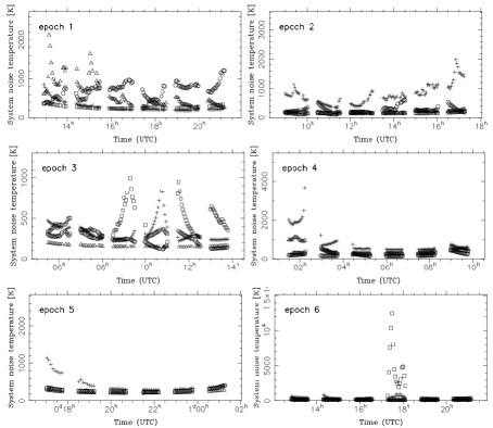
Figure 1: System noise temperature for all the observations. The horizontal axis is observing time in UTC, and the vertical axis is system noise temperature in Kelvin. Circles, triangles, squares, and crosses represent Mizusawa, Iriki, Ogasawara, and Ishigaki stations, respectively.

In our data reduction, we could not obtain uniform signal-to-noise ratio through all of the epochs because the atmospheric attenuation were unexpectedly highly variable dependent on observing season in Japan. In Table 1 and Figure 1, we show the variations of system noise temperatures for all the antennas.

Basically we followed a standard manner of spectral line VLBI data reductions with AIPS (NRAO) package. However, because of insufficient ($u$, $v$) coverage of the VERA observations, we found many confusing emission peaks due to the side-lobes coupled with still-not-perfect amplitude calibration. In such a situation, mapping accuracy can depend on the details of data reduction. Here we note the details of our data reduction in order to assure the reproducibility of our mapping results.

Table 1: Time average of the system noise temperature of each stations for all the epochs.

Epoch	Mizusawa [K]	Iriki [K]	Ogasawara [K]	Ishigaki [K]
epoch 1	692	596	280	289
epoch 2	242	230	181	799
epoch 3	240	161	428	328
epoch 4	205	479	311	834
epoch 5	276	234	283	443
epoch 6	137	117	1050	417

3.1 Visibility Calibrations

In order to get reliable images, we must perform calibrations of phase, amplitude, and bandpass characteristics of visibility data. For visibility-amplitude calibrations, we first performed the task ACCOR with SOLINT=0.1. Using auto-correlation spectra, the task ACCOR corrects amplitude errors in cross-correlation spectra suffered from sampling thresholds. Then we used the task APCAL to generate an amplitude calibration SN table, which includes the information of antenna gain curve (from GC table) and system noise temperatures (from TY table) of each station. Furthermore, we applied the amplitude solutions obtained from the self calibration method using the task CALIB.

For visibility-delay, rate, and phase calibrations, we used the task FRING with SOLINT=1.0 (SOLSUB=0.1) in order to obtain the clock offset and rate from the strong continuum source, J0530+13 inserted between S269 observing scans. As for fine phase calibrations, we relied on the self calibration solutions from the CALIB in AIPS at the last stage of calibrations (SOLINT=0.1, SOLSUB=0.05). The self calibrations were at first performed at the peak frequency channels corresponding to the ${V_{\rm LSR}}=19.5$ km s^-1(248 ch, 88 ch, 90 ch, 266 ch, 239 ch, and 240 ch in frequency at respective epochs). The frequency and velocity resolutions were common through all the observational epochs. Although these channels contained strong maser emissions, the maser structures were not a single spot but at least two spots with comparable intensities. The solutions of calibrations from these methods were applied to not only the reference channel but all of the velocity channels.

As for bandpass calibrations we used the task BPASS in AIPS with total power spectra of calibrator continuum sources and got the amplitude bandpass characteristics. After these calibrations, we performed corrections of velocity-shift due to diurnal rotation of the earth using the task CVEL in AIPS.

3.2 How to Make Maps

3.2.1 Search for Masing Regions

To find the whole region of H₂O maser emissions, instead of fringe rate mapping, we used wide area synthesis imaging with low spatial resolutions. We performed synthesis imaging of the $2\times 2$ arcseconds area in all velocity channels of four epoch’s data (the 1st, the 3rd, the 5th, and the 6th epochs). The $2\times 2$ arcseconds area was covered with $4096\times 4096$ grids. Namely, each cell size is about 0.5 mas. From these coarse maps, we selected positions for synthesis imaging with fine spatial resolution. We selected positions where the first CLEAN components of the different epochs’ data coincided with each other within 0.1 arcsecond. In addition to the positions, we added 0.3 arcseconds square areas around the three positions where strong maser emissions were found (around positions C, D, and E shown in Figure 9). We thus selected 42 of $100\times 100$ mas areas to be mapped with higher spatial resolution.

3.2.2 Fine Synthesis Imaging of the Selected 42 Areas

We mapped the 42 squares with $4096\times 4096$ grids. Each cell size is 24.4$\mu$ arcseconds. For the synthesis imaging, we used the task IMAGR in AIPS with parameters NITER=3000, GAIN=0.01, and FLUX=15 mJy. The selected minimum flux density level of a CLEAN component, FLUX=15 mJy is presumably lower than the array sensitivity. Because the absolute flux density of the data has an uncertainty due to insufficient amplitude calibrations, we used the lower level in order to achieve an adequate subtraction.

3.3 Measurements of Maser Positions

In order to avoid subjective selections of maser spots, we ran the task SAD in AIPS automatically with its default parameters. We divided the respective $4096\times 4096$ grid areas into 25 sub-areas ($4\times 4$ mas square), and ran the task SAD in each sub-area and measured maser spot positions. This selection method partially failed to select some maser positions around strong masers because such regions include not a few numbers of high level peaks due to the side-lobes. However, we adopted the automatic SAD selection to prioritize objectivity in selecting maser spots. By the SAD selection we found a lot of peak positions. The numbers of peaks with flux density $\geq 6\sigma$ are given in Table 2. Presumably, side-lobes or not real maser spots mingle among the selected peaks by the SAD method. It was quite difficult to select only real maser spots from these maps. To completely avoid selecting peaks that are not real, criteria other than their signal-to-noise ratios (SNR) are required.

Obs Epoch	Peak Number	$1\sigma$ Noise Level
	$(>6\sigma)$	(Jy/Beam)
1	238	$1.37$
2	354	$4.82\times 10^{-1}$
3	379	$4.88\times 10^{-1}$
4	660	$1.22$
5	177	$1.09$
6	789	$5.78\times 10^{-1}$

Table 2: Numbers of the maser emission peaks selected by the SAD method. $1\sigma$ noise levels were measured from the ${V_{\rm LSR}}=18.5$ km s^-1channel at the $100\times 100$ mas field centered at (980 mas, 370 mas) in the map of Figure 9.

4 Results

Section 4.1 shows the cross power spectra of the H₂O maser in the present data analysis. Sections 4.2 and 4.3 show the spatial distributions of the H₂O maser emissions and its time variation in the individual maser spot clusters and the whole area of S269. Relative proper motions of the maser clusters are presented in section 4.4. Here we define a “maser spot” as the origin of a maser emission in a single velocity channel map, and a “maser feature” as a group of maser spots with different velocities gathered at a common place. We also use the term “maser cluster” as a group of maser features with a common motion.

4.1 Cross power spectra of H₂O masers in S269

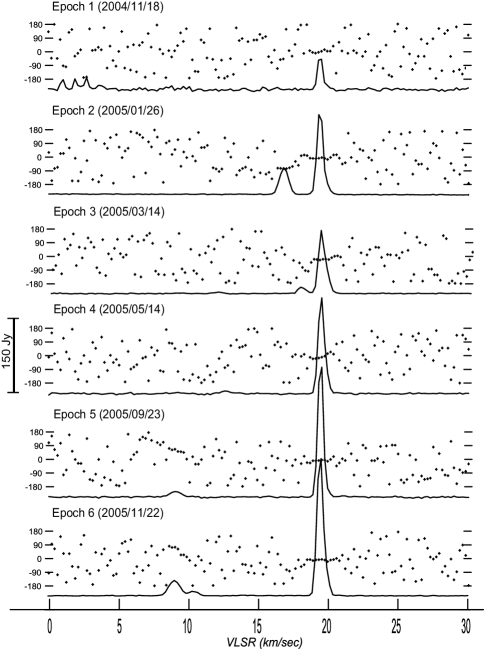
Figure 2: Cross power spectra of the H₂O maser emissions in S269 at all the epochs obtained from the integration of the entire body of data after calibrations for the Mizusawa–Iriki baseline. Because these amplitudes are obtained from scalar averaging of the cross-power spectra, the scale has some ambiguity. Several peaks seen between ${V_{\rm LSR}}$= 0 to 5 km s^-1at epoch 1 (top) are not from H₂O maser emissions, but due to artificial radio emissions. The dots show the phase variations with line of sight velocity channels. Phase value is shown in degree ranging within $\pm 180^{\circ}$.

Figure 2 shows the cross power spectra of the H₂O maser emissions in S269 obtained with the Mizusawa–Iriki baseline (1300 km length) for all the six epochs. It is important to note that there are complex maser emission peaks in the radial velocity range from 8 to 20 km s^-1, and that the line profile is changed on a time scale shorter than one year, as reported by Lekht et al. (2001a). The most prominent emission can be seen at ${V_{\rm LSR}}$ of 19.5 km s^-1, and the line profile of H₂O maser spectrum changes significantly in one year. Note also that there are several emission peaks in the spectra at ${V_{\rm LSR}}$ of 17 km s^-1at epoch 2, ${V_{\rm LSR}}$ of 18 km s^-1at epoch 3, and ${V_{\rm LSR}}$ from 8 to 11 km s^-1at epochs 5 and 6. The signal-to-noise ratio (SNR) of the cross power spectrum at epoch 1 seems worse than those at the other epochs. This is mainly because the system noise temperatures of these two stations at epoch 1 were unusually a factor of 2 to 5 higher than those at other epochs and also because the observing time of S269 was about half of those in other epochs.

In the cross power spectrum at epoch 1, there are several peaks between ${V_{\rm LSR}}=0$ to 5 km s^-1, but they are not maser emissions. This is due to strong artificial signals at Iriki station. We found the artificial signals at 21.233 GHz (corresponding to $V_{\mathrm{LSR}}$ = 35 km s^-1), 22.235 GHz (corresponding to $V_{\mathrm{LSR}}=0$ km s^-1), and 22.237 GHz (corresponding to $V_{\mathrm{LSR}}$ = $-22$ km s^-1) in sky frequency, one of which caused the peaks at ${V_{\rm LSR}}$ from 0 to 5km s^-1.

4.2 Arcsecond scale distribution of H₂O masers in S269

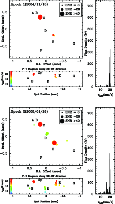
Figure 3: Spatial distributions of the H₂O maser groups of A to G in S269. The distributions at epochs 1 & 2. Panel top left: the distribution of the maser spots with SNR$\geq 8$. In group F, there is no maser spot with SNR$\geq 8$. Peaks around group C are not plotted because they are mostly side-lobes. Right panel: spectra composed from the plotted maser spots. Bottom left panel: position-velocity diagrams of the plotted maser spots cutting along the northeast-southwest.

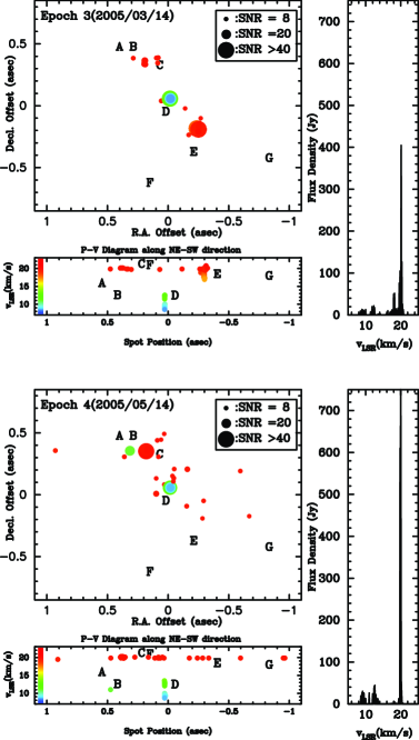
Figure 4: Continued. The distributions at epochs 3 & 4.

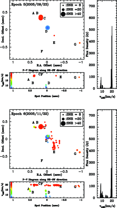
Figure 5: Continued. The distributions at epochs 5 & 6.

Figures 3, 4, and 5 show the spatial distribution of the maser spots and position-velocity diagrams for all the six epochs. We identified seven maser groups (A through G). All of them show strong time variation. At epoch 1, only group C was strong (${\rm SNR}>40$). C and E were strong at epoch 2, D and E at epoch 3, C and D at epochs 4 to 6. Groups C, E, F and G all lay in ${V_{\rm LSR}}$ ranging from 18 to 20 km s^-1. The maser emissions from ${V_{\rm LSR}}~{}=8$ to 14 km s^-1 came from a single group denoted as D. The distribution of masers was qualitatively consistent with the map obtained by Migenes et al. (1999). They identified four sources at 16.5, 17.3, 19.4 and 20.7 km s^-1, which roughly coincide with groups A, C, E and G. They used a fringe-rate mapping method to obtain the positions of the four peaks in their spectrum. Therefore, they did not obtain the velocity structures of the individual sources. The fact that they did not report the velocity distribution within each maser group does not mean the observed groups were single points.

4.3 Structure of individual maser groups

Figure 6 shows the internal maser structures of groups A to G. The structure of A is taken from epoch 6, that of B is from epoch 4, those of C, D, and E are from epoch 3, and those of F and G are from epoch 6. Each maser group consists of one or two features. One feature typically has a spatial size over 1 mas and a velocity range of 2 km s^-1. Groups D and E consist of two features, while other groups consist of one feature. As shown in the panel for group A, the typical beam size is $1.4\times 0.9$ mas. For maser spots in group C, SNR is higher than 100. From the high SNR, we can expect that the error of the relative position is small down to 0.01 mas. For other maser spots, SNR is in a range of 10–20. This implies that a possible position error is 0.1 mas or larger. Group C is the brightest among the clusters A-F, and it should correspond to the maser cluster studied in H2007. H2007 detected the maser spots with ${V_{\rm LSR}}$ from 19.0 to 20.1 km s^-1, which were distributed over an angular range of 0.4 mas in the east–west direction. While we detected from group C in wider velocity range of 18.8 to 21.4 km s^-1 as shown in Figure 6. As shown in Fig. 7 (a), the maser spots in the same velocity range as reported by H2007 show a more compact distribution within an angular range of 0.2 mas. We discuss the difference between the two maps in section 5.1.

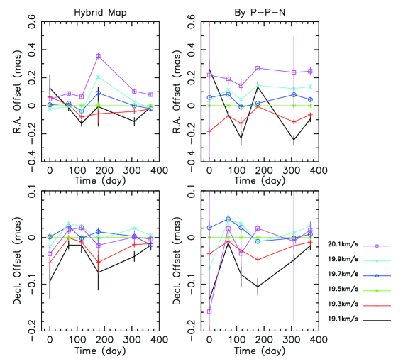
Figure 8: Positional offsets of the maser spots involved in group C with respect to the position of the maser spot with ${V_{\rm LSR}}=19.5~{}$km s^-1. Comparisons of our results from hybrid mapping and those from the P-P-N method: Left panels are from ours while right panels are from the P-P-N method. Top panels are for R. A. offsets while bottoms are for declination offsets.

The left two panels of Figure 8 show the relative positions of the maser spots in group C with respect to the position of the maser spot at ${V_{\rm LSR}}=$ 19.5 km s^-1. Positional deviations at epochs 1 and 4 are larger than those at other epochs: positions at epochs 2, 3, 5, and 6 are consistent with one another within the positional accuracy of 0.05 mas. Judging from the system noise temperatures, the large positional deviations at epochs 1 and 4 were caused by the bad atmospheric conditions as noted in section 2. The plot shows that change of relative positions of maser spots in the cluster reaches 0.5 mas between observational epochs (see section 4.1 on possible errors in the annual parallax).

4.4 Relative Proper Motions of Maser Clusters

Figure 10 shows the proper motions of maser clusters relative to the ${V_{\rm LSR}}=19.5$ km s^-1 spot in group C. First, we searched proper motions of maser spots from groups A to G (Figure 9). Among the selected peaks, we searched for relative proper motions of maser spots with the following three criteria.

1. Peaks which are higher than $20\sigma$ noise level at each epoch.

2. Peaks whose displacements are less than a corresponding proper motion of $3.5$ mas yr^-1.

3. Peaks whose velocity shifts are less than $0.5$ km s^-1.

For peaks in the two fields of groups F and G, where the maser spots were well isolated, we selected peaks which are higher than $7\sigma$ noise level at each epoch. Because these two maser groups show relatively weak emissions but the existence of the groups is certain, these masers cannot be neglected in order to investigate the internal motions of the masers in S269 regions. We found 22 sets of proper motions using the first criterion. Using the looser criterion on SNR, we found more 4 sets of proper motions and 1 set of proper motion from the two groups F and G respectively. In Table 3 we show the detected proper motions of maser spots with these criteria.

After detecting proper motions of maser spots, we combined all maser spots data showing common proper motions in order to obtain independent motions. First of all, from the proper motions data set, we omitted data using positions of epoch 1 and 4 as these two epochs were under fairly bad atmospheric conditions. We combined and averaged proper motions and velocities of maser spot data whose velocity difference was within 1 km s^-1 in order to derive independent motions of maser clusters.

Table 4 gives the parameters of derived proper motions of maser clusters. Apparently, the maser clusters in groups C, D, E and G form an arc-like structure with the proper motions implying an expanding shell. Since the number of clusters is limited, it is possible to judge that this structure and motion could be just a coincidence.

5 Discussion

We have re-analyzed the VERA archival data of S269. We found that (a) maser emissions in S269 are distributed over around 1.6 arcseconds, (b) the maser emissions are found from a wide radial velocity range between 8 and 20 km $s^{-1}$, (c) there are multiple maser groups in the 1.6 $\times$ 1.6 arcsecond area at around the radial velocity of 19.5 km s^-1, and (d) the structure of the brightest source (group C) is different from the single source reported in H2007. In section 5.1, we discuss the origin of the discrepancy in the obtained maser structure between our result and that of H2007. In section 5.2, we discuss the implication of the internal maser motions on the constraint on the galactic rotation curve of the Milky Way.

5.1 Comparison with the map of H2007

In Figure 7, we show the distribution of maser spots of group C and that of H2007, for the same epoch. Both show velocity gradients in the east-west direction, but H2007’s spots in the velocity range of ${V_{\rm LSR}}=19.0$ to 20.1 km s^-1 are distributed over 0.4 mas, while those in our result have a more compact distribution within 0.2 mas. We consider the possibility that the difference between our methods of analysis and those of H2007 caused the difference in the images. The primary difference between the two methods is that we have made the image from hybrid mapping, while H2007 used the phase-referenced data to determine the absolute positions of the maser spots. This difference of the mapping techniques themselves does not seem to cause significant differences in the determination of the internal structure. Rather, the reasons for the difference lie in differences in the treatment of the data.

We noted the following two major differences. First, H2007 did not find groups E and G, which are in the same velocity range as group C. Second, when they performed the analysis of the data, they applied corrections for the atmospheric delays of stations to the visibility data in order to obtain a reasonable result. They noted: “To calibrate them, residual zenith delays were estimated as a constant offset that maximizes the coherence of the phase-referenced map. Typical residuals of zenith delay are 1 to 5 cm, but in the worst case (during the summer at Ishigaki-jima station) it was as large as 20 cm”.

They maximized the coherence by adjusting the residual atmospheric excess path-length, $L_{s}$ of individual stations, under the following assumptions:

1. The excess path-length $\delta L_{S}$ to be adjusted at station S is $\delta L_{S}=L_{S}\times~{}(\sec~{}Z_{\rm S269}-\sec~{}Z_{\rm ref})$, where $Z_{X}$ is the zenith angle of source X at station S and $L_{S}$ is the residual atmospheric zenith delay at station S.

2. The residual atmospheric zenith delay $L_{S}$ is constant during one observational session.

3. The correct estimate of the residual excess path-length $L_{S}$ gives the correct map of S269.

We investigated how these assumptions can change the map. For this purpose we created a map using the method which is effectively equivalent to that used in H2007. The difference between the standard imaging method and this is summarized as follows. In the standard imaging method one uses fine solutions of both amplitude and phase from self-calibration with an optimized model image, however here we used self-calibration only for phase solutions using a point as the image model. Calibration of phase $\phi$ is equivalent to that of excess path-length $L$ due to the equation $\phi=2\pi L/\lambda$ (where $\lambda$ is observing wavelength). We assumed that the source in one velocity channel has a single point when we performed the phase self-calibration. We limited the imaging area to a narrow region ($100\times 100$ mas span). If they performed wide-area imaging, they should have found multiple sources as we found. (Hereafter we call the map obtained by the above mentioned method as the PPN map: Phase-only self-calibration with an one-Point model and Narrow field mapping). In Figure 7 we show the PPN map overlaid with the result of H2007. We can see that the PPN map reproduces the main feature of the H2007 map. In particular, the width of the distribution of maser spots is 0.4 mas for both results. We ignored the presence of multiple sources and performed only the phase calibration in the PPN map. This suggests that the result of H2007 is affected by the imaging area and choice of the calibration method.

Figure 8 shows the time variation of the relative positions of the maser spots in group C with respect to that at the velocity of 19.5 km s^-1 revealed by the standard mapping and the PPN method. It is clearly seen that the distribution of the spots along the right ascension in the PPN is $\sim 0.1$ mas wider than that in the standard mapping method, so that the difference between the two as shown in Figure 7 can be reproduced for all the epochs. It is worth noting that, assuming that the standard mapping method produce true maser emission images better than the PPN method because the PPN method uses a single point source model even if the structure is complicated, the positional shift seen in the PPN map causes an astrometric error, which depends on the source structure.

Provided that this positional shift have the same direction and the same quantity for all the epochs, following astrometric analysis to obtain annual parallaxes and proper motions can make a correct estimation of the annual parallax. On one hand, if the positional shift have a one-year periodical variation, the derived annual parallax may have a bias of 0.1 mas in the worst case. If the positional shift appears randomly, the annual parallax error could be between $0-0.1$ mas by chance. From our comparison between the standard mapping method and the PPN method, and between the PPN method and the map shown in H2007, we suspect that H2007 applied a simple source model in their analysis which does not include a widely distributed maser emission as shown in this report, so that their annual parallax have a hidden error of 0.1 mas in the worst case.

5.2 Effects of the internal motions in S269 on the Galactic dynamics

One of the most important claims in H2007 is that motion and distance to S269 give a strong constraint on the shape of the outer rotation curve of the Milky Way: the difference of rotational velocities at the Sun and at S269 (which is claimed to be located at 13.1 kpc away from the Galactic center) is less than 3%. However, our reanalysis suggests that we cannot give that strong constraint on the outer rotation curve only by the VERA observation of S269, if we consider the complicated internal structures of maser clusters and their motions as well as their time variability.

We calculated the $UVW$ velocities of the independent maser clusters using relative proper motions and radial velocities, assuming that H2007 velocity corresponds to that of the ${V_{\rm LSR}}=19.5$ km s^-1 in the maser spot in group C. The results are summarized in Table 5. The average UVW of these maser clusters in S269 is ($4.4\pm 6.1,-16.7\pm 18.4,12.2\pm 18.7$ km s^-1). Assuming that H2007 obtained the correct distance to S269, the rotational velocity at 13 kpc is $183\pm 19.4$ km s^-1.

The rotational velocity at 13 kpc, $183\pm 19.4$ km s^-1, is consistent with other measurements. Owing to the large internal motion of masers in S269, the observed proper motion of S269 with respect to the Local Standard of Rest cannot give a strong constraint on kinematics of the outer part of the Galaxy, in contrast to the claim by H2007. Taking into account the internal motion of $\sim 20$km s^-1, the rotational velocity of S269 is consistent with other previous observations outside of the solar circle (Sofue et al., 2009).

5.3 Difficulties in VLBI astrometry using H₂O masers in star forming regions

VLBI astrometry using H₂O maser sources has made great progress in decades as a powerful tool to investigate structures and dynamics of the Milky Way Galaxy (e.g. Reid et al., 2009; Sato et al., 2010). However, our result presented here illuminates essential difficulties in this methodology. Major intrinsic problems are: 1) H₂O masers in star forming regions are not necessarily located in the ‘center of mass’ of the objects, 2) the masers are not in general “point ” sources, and their distributions are time-variable, and 3) they often show complicated internal motions. Additionally, the different results between H2007 and the present work suggested that the data calibration in VLBI observations of star forming regions is not straightforward, and still need improvement.

One should also note that the shapes of H₂O masers are not point-like and their spatial extent are often comparable to observational beam size. For example, we found that average size of H₂O masers in S269 is $0.72\pm 0.50$ mas (HPBW) based on a Gaussian shape fitting, which is comparable to the VERA synthesized beam size at 22 GHz (Figure 6). The distributions of masers often change between observational epochs, which brings additional errors on position of the objects.

Moreover, H₂O maser sources in a star forming region often show internal motions, i.e. spots apparently moves in terms of the center of mass of the region. Such internal motions are typically a few tens of km s^-1, and therefore it is hard to estimate the kinematic motions of the objects in the Galaxy. This could be solved by introducing a model of internal motions (e.g. expanding outflows) of maser spots (e.g. Imai et al., 2000; Asaki et al., 2010). However, this suggests that a large enough number of spot motions should be measured over many years, and that the motions are often too complicated to be fitted by a simple kinematic model.

Finally, one should note that the astrometric results of star forming regions using the VLBI technique is still carefully considered. For example, in S269, as shown in section 5.1, the difference of data calibration and the assumption for measurement may cause up to $0.1mas$ ambiguity in the astrometric results. Although it would be hard to overcome the intrinsic difficulties in H₂O masers of star forming regions, one could reduce errors in astrometry by searching maser spots as many as possible in a large enough area, and those spots should be observed over many years.

6 Summary

We have reanalyzed VERA archival data of S269, and found several maser clusters distributed over 1.6 arcseconds on the sky. The distribution of maser spots in the strongest maser feature differs from that obtained by H2007 with $\sim 0.2$ mas. We confirmed that this discrepancy is caused by unrealistic assumptions and insufficient procedures of analysis. If we assume only a single spot in one velocity channel and perform self phase-only calibration, the results of H2007 are reproduced. We also found that the relative proper motions and radial motions of multiple maser clusters are quite large, and therefore the absolute proper motion of S269 does not pose a tight constraint on the rotation curve of the Milky Way as was claimed by H2007. Our analysis also shows that change of relative positions of maser spots in the cluster reaches 0.1 mas or larger between observational epochs. All these results imply that the annual parallax of S269 could not be determined within an error of $\sim$ 0.1 mas using assumptions of a single point source model for such widely distributed maser sources.

Thus the maser astrometry should be performed carefully with consideration about structure and the time-variation of maser source. The internal motions of maser clusters among the system also be considered for Galactic astrometry. The VLBI astrometric accuracy depends on the way of data analysis. Thus, the details, as well as the results, should be noted clearly for refinement by future ages.

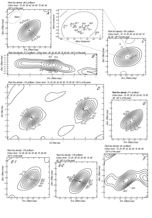
Figure 6: Velocity structures of the respective maser groups in S269. Velocity integrated maser features are expressed with contour maps. Contours are drawn at each 10 % of the peak intensity. Positions of velocity components are plotted by cross marks, denoting numbers indicating the ${V_{\rm LSR}}$ velocities. The structure of A is from epoch 6, that of B is from epoch 4, those of C, D, &E are from epoch 3, and those of F & G are from epoch 6. The typical restoring beam shape ($1.4\times 0.9$ mas) is shown at top left in panel A.

Figure 7: Comparison of the maser spot distribution with that of H2007. (a) Comparison of our results and that of H2007. The crosses represent the position of the each maser spot in group C obtained from data analysis using the hybrid mapping method. From our map, we detected maser spots for a wider velocity range of 18.8 to 21.4 km s^-1in the maser group C, but here for comparison we plot the spots limited in the range from ${V_{\rm LSR}}=19.1$ to$~{}20.1$ km s^-1. The filled circles are results reported by H2007, and the color represents the radial velocity. Two maps are aligned at the spot position of ${V_{\rm LSR}}=20.1$ km s^-1. (b) Comparison of the results from the PPN method and that of H2007. The crosses show the position of velocity component ${V_{\rm LSR}}=19.1$ to$~{}20.1$ km s^-1from our reproduction image by the PPN method.

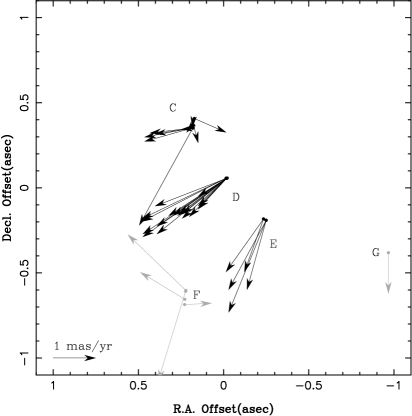
Figure 9: Relative proper motions of the H₂O maser spots in S269 with respect to the maser spot position with ${V_{\rm LSR}}$ of 19.5 km s^-1. The proper motions shown by black arrows are detection with SNR$\geq 20$ from groups C, D, and E. Those shown by gray arrows are detection’s with $SNR\geq 7$ from the weaker groups F (220 mas, -600mas) and G (-970 mas, 380 mas).

Figure 10: Relative proper motions of the independent 9 H₂O maser clusters in S269. The maps of the 6 observational epochs are aligned using the strong maser spot position in the maser group C at ${V_{\rm LSR}}=19.5$ km s^-1.

Table 3: Relative Proper Motions of Maser Spots.

No		Time	Velocity	Relative Position		Intensity		Size	Proper Motion		Overlap
			$v_{\rm LSR}$	$\alpha$	$\delta$			HPBW	$\mu$	$PA$
		(day)	(km s-1)	(mas)	(mas)	(Jy)	(S.N.R.)	(mas)	(mas yr-1)	(∘)
1…1	D1	309	8.3	-18.98	57.14	278	25.5	0.58
…2	D1	369	8.3	-18.87	57.04	352	60.9	0.50	0.94	-44
2…1	D1	309	8.5	-18.98	57.14	465	42.6	0.53
…2	D1	369	8.5	-18.87	57.02	626	108.3	0.37	0.99	-47
3…1	D1	309	8.7	-19.04	57.14	696	63.9	0.31
…2	D1	369	8.7	-18.93	57.02	977	169.0	0.13	0.99	-47	a
4…1	${}^{~{}~{}}$	116	8.9	-19.65	57.61	125	25.6	0.70
…2	${}^{~{}~{}}$	177	8.9	-19.38	57.42	252	20.6	0.59	2.00	-35
…3	D1	309	8.9	-19.04	57.14	934	85.7	0.15	1.46	-37	b
…4	D1	369	8.7	-18.93	57.02	977	169.0	0.13	1.35	-39	a
5…1	${}^{~{}~{}}$	116	9.2	-19.71	57.61	116	23.7	0.70
…2	${}^{~{}~{}}$	177	9.1	-19.43	57.39	292	23.9	0.50	2.11	-39	c
…3	D1	309	8.9	-19.04	57.14	934	85.7	0.15	1.55	-35	b
…4	D1	369	8.7	-18.93	57.02	977	169.0	0.13	1.41	-37	a
6…1	${}^{~{}~{}}$	116	9.4	-19.76	57.61	109	22.4	0.70
…2	${}^{~{}~{}}$	177	9.1	-19.43	57.39	292	23.9	0.50	2.38	-34	c
…3	${}^{~{}~{}}$	309	8.9	-19.04	57.14	934	85.7	0.15	1.63	-33	b
7…1	${}^{~{}~{}}$	116	9.6	-19.82	57.64	101	20.6	0.64
…2	${}^{~{}~{}}$	177	9.5	-19.49	57.40	255	20.9	0.52	2.42	-35
…3	D2	309	10.0	-19.26	57.13	277	25.4	0.28	1.42	-42
…4	D2	369	10.0	-19.20	57.01	451	78.0	0.36	1.27	-46
8…1	D2	309	10.2	-19.37	57.08	263	24.2	0.67
…2	D2	369	10.2	-19.26	57.01	512	88.5	0.44	0.80	-32	d
9…1	D2	309	10.4	-19.54	57.11	283	25.9	0.48
…2	D2	369	10.2	-19.26	57.01	512	88.5	0.44	1.82	-21	d
10…1	${}^{~{}~{}}$	116	12.3	-14.98	56.92	218	44.7	0.73
…2	${}^{~{}~{}}$	177	12.5	-14.65	56.74	418	34.2	0.60	2.23	-27	e
11…1	${}^{~{}~{}}$	116	12.5	-14.98	56.90	130	26.6	0.69
…2	${}^{~{}~{}}$	177	12.5	-14.65	56.74	418	34.2	0.60	2.20	-26	e
12…1	E1	69	18.2	-234.74	-182.96	112	23.2	0.51
…2	E1	116	18.2	-234.68	-183.12	435	89.1	0.65	1.33	-70	h
13…1	E1	69	18.4	-234.79	-182.96	110	22.8	0.31
…2	E1	116	18.2	-234.68	-183.12	435	89.1	0.65	1.53	-55	h
14…1	${}^{~{}~{}}$	0	19.3	180.82	350.61	321	23.4	2.33
…2	${}^{~{}~{}}$	369	19.2	181.10	350.59	709	122.7	1.39	0.28	-6
15…1	${}^{~{}~{}}$	0	19.5	176.43	367.39	400	29.2	0.60
…2	${}^{~{}~{}}$	369	19.2	176.32	366.97	247	42.8	1.32	0.43	-105
16…1	E2	69	19.7	-250.18	-190.67	154	32.0	0.17
…2	E2	116	19.7	-250.07	-190.95	265	54.3	0.21	2.34	-68
17…1	${}^{~{}~{}}$	177	19.9	172.04	407.95	311	25.4	1.28
…2	${}^{~{}~{}}$	309	20.1	171.76	407.83	364	33.4	2.18	0.82	-156
18…1	E2	69	19.9	-250.13	-190.70	187	38.7	0.25
…2	E2	116	20.1	-250.07	-190.91	326	66.6	0.60	1.70	-75	f
19…1	${}^{~{}~{}}$	0	19.9	179.71	352.89	614	44.8	0.85
…2	${}^{~{}~{}}$	69	19.9	179.93	352.83	561	116.4	0.68	1.18	-16
…3	${}^{~{}~{}}$	177	20.1	180.20	352.83	810	66.3	0.79	1.03	-7	g
…4	${}^{~{}~{}}$	369	19.5	180.99	350.57	676	116.9	1.92	2.62	-61
20…1	${}^{C~{}}$	69	19.9	181.82	370.31	168	34.8	0.65
…2	${}^{C~{}}$	309	19.9	181.82	370.27	293	26.9	0.50	0.07	-83
…3	${}^{C~{}}$	369	19.9	181.93	370.17	192	33.3	1.33	0.23	-52
21…1	E2	69	20.1	-250.18	-190.70	159	32.9	0.20
…2	E2	116	20.1	-250.07	-190.91	326	66.6	0.60	1.86	-62	f
22…1	${}^{~{}~{}}$	0	20.1	179.77	352.91	471	34.3	1.14
…2	${}^{~{}~{}}$	69	20.1	179.98	352.86	339	70.2	0.86	1.16	-11
…3	${}^{~{}~{}}$	177	20.1	180.20	352.83	810	66.3	0.79	0.92	-9	g
23…1	${}^{~{}~{}}$	177	20.1	223.10	-608.20	86	7.0	0.10
…2	${}^{~{}~{}}$	369	20.1	223.44	-609.30	57	9.9	1.80	2.21	-73
24…1	F1	116	20.1	229.32	-685.79	39	8.0	0.29
…2	F1	369	19.9	228.88	-685.77	46	7.9	1.42	0.64	177
25…1	F2	116	20.1	227.88	-654.77	37	7.6	0.75
…2	F2	369	19.9	228.60	-654.33	49	8.5	1.06	1.23	31
26…1	F3	116	20.1	220.82	-602.79	40	8.1	0.76
…2	F3	369	19.9	221.77	-601.88	50	8.7	0.93	1.90	44
27…1	${}^{G~{}}$	309	18.2	-967.49	-380.66	119	10.9	0.47
…2	${}^{G~{}}$	369	18.2	-967.49	-380.82	77	13.3	0.30	0.96	-90

Note. — Column 1: Detection of proper motion. Subscription indicates the affiliation to the maser cluster. Column 2: Observing day, Column 3: Velocity of the spot, Column 4: $\alpha$ position of the spot. Column 5: $\delta$ position of the spot. The coordinate system is the same as in Figure 9. Column 6: Intensity in Jansky. Column 7: Signal to noise ratio of the spot. Column 8: Size of the maser spot(HPBW). Column 9: Dimension of the proper motion. Column 10: Position angle of the direction of the proper motion. Column 11: Overlap selection of the maser spot selection.

Table 4: Relative Proper Motions of Independent Clusters.

Cluster	Velocity	Relative Position		Intensity		Proper Motion
	$v_{\rm LSR}$	$\alpha$	$\delta$			$\mu_{\alpha}$	$\mu_{\delta}$	$\mu$
	(km s-1)	(mas)	(mas)	(Jy)	(S.N.R.)	(mas yr-1)	(mas yr-1)	(mas yr-1)
1. D1	8.7	-18.96	57.09	722	98	0.68	-0.71	0.98
2. D2	10.2	-19.32	57.06	383	55	0.90	-0.62	1.15
3. E1	18.3	-234.72	-183.04	273	56	0.67	-1.25	1.43
4. E2	19.9	-250.12	-190.80	236	49	0.74	-1.81	1.97
5. C	19.9	181.86	370.25	218	32	0.34	-0.36	0.51
6. F1	20.0	229.10	-685.78	43	8	-0.64	0.03	0.64
7. F2	20.0	228.24	-654.55	43	8	1.05	0.64	1.22
8. F3	20.0	221.30	-602.33	45	8	1.37	1.31	1.89
9. G	18.2	-967.49	-380.74	98	12	0.00	-0.96	0.96

Note. — Column 1: Cluster Name, Column 2: Velocity of the cluster, Column 3: Mean $\alpha$ position of the cluster, Column 4: Mean $\delta$ position of the cluster. The coordinate system is the same as in Figure 10. Column 7: Mean intensity in Jansky, Column 8: Mean signal to noise ratio of the cluster, Column 9: $\alpha$ component of the proper motion, Column 10: $\delta$ component of the proper motion, Column 11: Dimension of the proper motion,

Table 5: Peculiar motions (deviation from a galactic circular rotation) of each maser cluster in S269. $U$, $V$, and $W$ [km s^-1] are three components of peculiar motions. $U$ is toward the Galactic center, $V$ is toward Galactic rotation, and $W$ is toward the North Galactic Pole. Galactic radius and circular rotation of the LSR are assumed to be $R_{0}=8.0~{}{\rm kpc}$ and $\Theta_{0}=200~{}$km s^-1. The flat rotation curve is assumed. The solar motion relative to the LSR is and $(U_{\odot},V_{\odot},W_{\odot})=(10.00,5.25,7.17)~{}$km s^-1(Dehnen and Binney, 1998),

		relative to $S269_{H2007}$			DB98
Cluster	$v_{\rm LSR}$	$\mu_{\alpha}$	$\mu_{\delta}$		U	V	W
	km s-1	mas yr-1	mas y$r^{-1}$		km s-1	km s-1	km s-1
$S269_{H2007}$	$19.60\pm 0.25$	_	_		$-0.1\pm~{}0.2$	$-0.6\pm~{}0.2$	$~{}-4.5\pm~{}0.1$
S269 C	$19.9\pm 0.0$	$~{}0.34\pm 0.47$	$-0.36\pm 0.42$		$~{}1.7\pm~{}0.8$	$-14.9\pm~{}5.6$	$~{}~{}9.4\pm 10.3$
S269 D1	$8.7\pm 0.2$	$~{}0.68\pm 0.00$	$-0.71\pm 0.03$		$14.7\pm~{}0.2$	$-24.6\pm~{}0.2$	$~{}13.0\pm~{}0.1$
S269 D2	$10.2\pm 0.2$	$~{}0.90\pm 0.70$	$-0.62\pm 0.18$		$13.1\pm~{}1.2$	$-25.5\pm~{}8.3$	$~{}18.8\pm 15.4$
S269 E1	$18.3\pm 0.1$	$~{}0.67\pm 0.31$	$-1.25\pm 0.00$		$~{}7.4\pm~{}0.5$	$-37.8\pm~{}3.7$	$~{}~{}6.0\pm~{}6.8$
S269 E2	$19.9\pm 0.2$	$~{}0.74\pm 0.25$	$-1.81\pm 0.30$		$~{}8.3\pm~{}0.5$	$-51.0\pm~{}3.0$	$~{}~{}0.8\pm~{}5.5$
S269 F1	$20.0\pm 0.2$	$-0.64~{}~{}~{}~{}~{}~{}~{}~{}$	$~{}0.03~{}~{}~{}~{}~{}~{}~{}$		$-1.4\pm~{}0.2$	$~{}~{}5.1\pm~{}0.2$	$~{}-7.5\pm~{}0.1$
S269 F2	$20.0\pm 0.2$	$~{}1.15~{}~{}~{}~{}~{}~{}~{}~{}$	$~{}0.64~{}~{}~{}~{}~{}~{}~{}$		$-1.4\pm~{}0.2$	$~{}-2.9\pm~{}0.2$	$~{}39.1\pm~{}0.1$
S269 F3	$20.0\pm 0.0$	$~{}1.37~{}~{}~{}~{}~{}~{}~{}~{}$	$~{}1.31~{}~{}~{}~{}~{}~{}~{}$		$-3.8~{}~{}~{}~{}~{}~{}~{}~{}$	$~{}~{}8.9~{}~{}~{}~{}~{}~{}~{}~{}$	$51.9~{}~{}~{}~{}~{}~{}~{}$
S269 G	$18.2\pm 0.0$	$~{}0.00~{}~{}~{}~{}~{}~{}~{}~{}$	$-0.96~{}~{}~{}~{}~{}~{}~{}$		$~{}5.4~{}~{}~{}~{}~{}~{}~{}~{}$	$-23.5~{}~{}~{}~{}~{}~{}~{}~{}$	$-5.2~{}~{}~{}~{}~{}~{}~{}$
average					$~{}4.4\pm~{}6.1$	$~{}-16.7\pm 18.4$	$~{}12.2\pm 18.7$

Appendix A Closure Phase of the ${V_{\rm LSR}}=19.5$ km s^-1channel

To demonstrate the complex structure at the ${V_{\rm LSR}}=19.5$ km s^-1channel from visibility data, here we show the closure phases of the ${V_{\rm LSR}}=19.5$ km s^-1channel, which was used for the astrometry by H2007. We found non-zero phase values in all the observational epochs (Figure 11). Non-zero closure phase indicates the existence of a complex structure. Closure phase $\Phi_{ABC}$ of a triangle composed of antennas A, B, and C is defined as follows.

$$\Phi_{ABC} \equiv \theta_{AB}^{obs}+\theta_{BC}^{obs}+\theta_{CA}^{obs}$$

where, $\theta_{AB}^{obs}=\theta_{AB}+(\phi_{A}-\phi_{B})$, $\theta_{BC}^{obs}=\theta_{BC}+(\phi_{B}-\phi_{C})$ , and $\theta_{CA}^{obs}=\theta_{CA}+(\phi_{C}-\phi_{A})$. $\theta_{XY}^{obs}$ is the observed fringe phase of the baseline between stations X and Y. $\phi_{X}$ is antenna based phase error. $\theta_{XY}$ is the intrinsic phase due to the observed source structure. If we substitute these in the equation,

$$\Phi_{ABC} = \theta_{AB}^{obs}+\theta_{BC}^{obs}+\theta_{CA}^{obs}$$

$$= \theta_{AB}+(\phi_{A}-\phi_{B})$$

$$+ \theta_{BC}+(\phi_{B}-\phi_{C})$$

$$+ \theta_{CA}+(\phi_{C}-\phi_{A})$$

$$= \theta_{AB}+\theta_{BC}+\theta_{CA}$$

In the closure phase $\Phi_{ABC}$, the antenna based phase errors are canceled, and the value of $\Phi_{ABC}$ is defined only by the phases due to the structure of the observed source. (Noted that a baseline based error, if such exists, is not canceled.) The closure phase is an observable quantity, totally free from instrumental delay or phase error at respective antennas, and is defined only by the structure of the observed source. The closure phase is very sensitive to asymmetry of the structure. A source whose structure is point symmetric yields zero closure phases for any array geometry. Conversely, the closure phase of an asymmetric source is non-zero (Jennison, 1958; Pearson&Readhead, 1984).

None of the structures of the H₂O masers at the ${V_{\rm LSR}}=19.5$ km s^-1channel were any kind of point symmetric structure including a single point. These closure phases also show time variations between the observational epochs, reflecting the structure changes in the velocity channel.

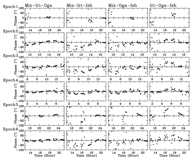
Figure 11: Closure phases of the channel, ${V_{\rm LSR}}=19.5$ km s^-1at the 6 observational epochs . From left to right, those of the four triangles, Mizusawa-Iriki-Ogasawara, Mizusawa-Iriki-Ishigaki, Mizusawa-Ogasawara-Ishigaki, and Iriki-Ogasawara-Ishigaki are shown. Every closure phase is from 7.0 min integration.

References

- Asaki et al. (2010) Asaki, Y., Deguchi, S., Imai, H., Hachisuka, K., Miyoshi, M., Honma, M. 2010, ApJ, 21, 266
- Baba et al. (2009) Baba, J., Asaki, Y., Makino, J., Miyoshi, M., Saitoh, T., Wada, K. 2009, ApJ, 706, 471
- Bertin & Lin (1996) Bertin, G., & Lin, C. C. 1996, Spiral structure in galaxies a density wave theory, Cambridge, MA MIT Press, Physical description x, 271
- Cesaroni (1990) Cesaroni, R. 1990, A&A, 233, 513
- Dehnen and Binney (1998) Dehnen, W., & Binney, J. 1998, MNRAS, 298, 387
- Genzel et al. (1977) Genzel, R., & Downes, D. 1977, A&AS, 30, 145
- Gwinn et al. (1992) Gwinn, C. R., Moran, J. M., & Reid, M. J. 1992, ApJ, 393, 149
- Honma et al. (2007) Honma, M., Bushimata, T., Choi, Y. K., Hirota, T., Imai, H., Iwadate, K., Jike, T., Kameya, O., Kamohara, R., Kan-Ya, Y., Kawaguchi, N., Kijima, M., Kobayashi, H., Kuji, S., Kurayama, T., Manabe, S., Miyaji, T., Nagayama, T., Nakagawa, A., Oh, C. S., Omodaka, T., Oyama, T., Sakai, S., Sato, K., Sasao, T., Shibata, K. M., Shintani, M., Suda, H., Tamura, Y., Tsushima, M., & Yamashita K. 2007, PASJ, 59, 889
- Imai et al. (2000) Imai, H., Kameya, O., Sasao, T., Miyoshi, M., Deguchi, S., Horiuchi, S., Asaki, Y. 2000, ApJ, 538, 751
- Jennison (1958) Jennison, R. C. 1958, MNRAS, 118, 276
- Kobayashi et al. (2008) Kobayashi, H., Kawaguchi, N., Manabe, S., Shibata, K. M., Honma, M., Tamura, Y., Kameya, O., Hirota, T., Jike, T., Imai, H., & Omodaka, T. 2008, In A Giant Step: from Milli- to Micro-arcsecond Astrometry, Proceedings of the International Astronomical Union, IAU Symposium, 248, 148
- Lekht et al. (2001a) Lekht, E. E., Pashchenko, M. I., & Berulis, I.I. 2001, Astronomy Reports, 45, 949 (Translated from Astronomicheski.. Zhurnal, 78, 1081)
- Lekht et al. (2001b) Lekht, E. E., Silant’ev, N. A., Mendoza-Torres, J. E., Pashchenko, M. I., & Krasnov, V. V. 2001, A&A, 377, 999
- Lin & Shu (1964) Lin, C. C.,& Shu, Frank H. 1964, ApJ, 140, 646
- Lo & Burke (1973) Lo, K. Y., & Burke, B. F. 1973, A&A, 26, 487
- Migenes et al. (1999) Migenes, V., Horiuchi, S., Slysh, V. I., Val’tts, I. E., Golubev, V. V., Edwards, P. G., Fomalont, E., Okayasu, R.,, Diamond, P. J., Umemoto, T., Shibata, K. M., & Inoue, M. 1999, ApJS, 123, 487
- Niinuma et al. (1982) Niinuma, K., Nagayama, T., Hirota, T., Honma, M., Motogi, K., Nakagawa, A., Kurayama, T., Kan-ya, Y., Kawaguchi, N., Kobayashi, H., & Ueno, Y. 2010, accepted to PASJ
- Oh et al. (2010) Oh, C. S., Kobayashi, H., Honma, M., Hirota, T., Sato, K., Ueno, Y. 2010, PASJ, 62, 101
- Pearson&Readhead (1984) Pearson, T. J.,& Readhead, A. C. S. 1984, ARAA, 22, 97
- Reid et al. (1988) Reid, M. J., Schneps, M. H., Moran, J. M., Gwinn, C. R., Genzel, R., Downes, D., Roennaeng, B. 1988, ApJ, 330, 809
- Reid et al. (2009) Reid, M. J., Menten, K. M., Zheng, X. W., Brunthaler, A., Moscadelli, L., Xu, Y., Zhang, B., Sato, M., Honma, M., Hirota, T., Hachisuka, K., Choi, Y. K., Moellenbrock, G. A., Bartkiewicz, A. 2009, ApJ, 700, 137
- Rygl et al. (2008) Rygl, K. L. J., Brunthaler, A., Menten, K. M., Reid, M. J., van Langevelde, H. 2008, Proceedings of the 9th European VLBI Network Symposium on the role of VLBI in the Golden Age for Radio Astronomy and EVN Users Meeting, 58
- Rygl et al. (2010) Rygl, K. L. J., Brunthaler, A., Reid, M. J., Menten, K. M., van Langevelde, H. J., Xu, Y. 2010, A&A, 511, A2
- Sato et al. (2010) Sato, M., Reid, M. J., Brunthaler, A.,& Menten, K. M. 2010, ApJ, 720, 1055
- Sofue et al. (2009) Sofue, Y., Honma, M., & Omodaka, T. 2009, PASJ, 61, 227
- Wada, Baba, & Saitoh (2011) Wada, K., Baba, J., & Saitoh, T.R. in prep.
- White et al. (1979) White, G. J., & Macdonald, G. M. 1974, MNRAS98, 589