Beyond the constraints underlying Kolmogorov-Johnson-Mehl-Avrami theory related to the growth laws

Abstract

The theory of Kolmogorov-Johnson-Mehl-Avrami (KJMA) for phase transition kinetics is subjected to severe limitations concerning the functional form of the growth law. This paper is devoted to side step this drawback through the use of correlation function approach. Moreover, we put forward an easy-to-handle formula, written in terms of the experimentally accessible actual extended volume fraction, which is found to match several types of growths. Computer simulations have been done for corroborating the theoretical approach.

1 Introduction

The Kolmogorov-Johnson-Mehl-Avrami (KJMA) model [1, 2, 3] finds application in a vast ambit of scientific fields which ranges from Thin Film Growth to Materials Science [4, 5, 6, 7, 8, 9, 10, 11] to Biology and Pharmacology [12, 13], let alone the Applied Probability Theory [14, 15]. In the majority of these studies the authors made use of a simplified version of the KJMA formula: the stretched exponential $X(t)=1-\exp(-at^{n})$, where $X$ is the fraction of the transformed phase, $a$ and $n$ (the latter known as Avrami’s exponent) being constants. The model, in principle, is simple because it rests on a Poissonian stochastic process of points in space, to which a growth law is attached. In fact, owing to the Poissonian process, the nucleation takes place everywhere in the space i.e. also in the already transformed phase. This partially fictitious nucleation rate ($I(t)$), for we are dealing with a Poissonian process, is linked to the actual (real) nucleation rate ($I_{a}(t)$) according to: $I_{a}(t)=I(t)[1-X(t)]$, where $X(t)$ is the transformed fraction. The growth law transforms each point in a nucleus of radius $R(t)$, $t$ stands for time. The pair, ”points’ generation” and ”growth law”, is a key quantity of the theory. It happens that the KJMA model fails for time-dependent points generation rate (i.e. nucleation rate) associated with diffusional-type growth laws [16],[17]. In particular, let us define two classes of growth laws: i) $d^{2}R/dt^{2}\geq 0$ and ii) $d^{2}R/dt^{2}<0$. The KJMA model is suitable for describing the first class of growths and for this reason we named it KJMA-compliant as opposite to the second to which we attach the adjective KJMA-non-compliant. The reason for that is due to the particular stochastic process taken into account. As a matter of fact, the Poissonian process requires that points can be generated everywhere throughout the space independently of whether the space is, because of growth, already transformed or not. Points generated in the already transformed space are named phantoms after Avrami. It goes without saying that, in the case of KJMA-compliant growths, phantoms do not contribute to the true transformed fraction, i.e. they are just virtual points whose only role is to simplify the mathematics [18]. On the other hand, in the KJMA-non-compliant growths phantoms may contribute to the phase transition through the non-physical ”overgrowth” events [3]. Incidentally, it is worth noticing that the KJMA-non-compliant growths and KJMA-compliant growths are indistinguishable if associated with simultaneous nucleation [19].

According to what has been said, one can summarize saying that the concept of phantom implies the existence of the two classes of growths.

One has to bring in mind that the above stretched exponential expression ( $X(t)=1-\exp(-at^{n})$) is the exact solution of the kinetics only in the case $I(t)=constant$ and $I(t)\sim\delta(t)$, $I$ being the nucleation rate and $\delta(t)$ Dirac’s delta function, provided the growth is according to a power law. In general, the term $at^{n}$ is a simple way to approximate the convolution product between the nucleation rate (phantom included) and the nucleus volume. This convolution is the ”extended” transformed fraction and takes into account the contribution of phantoms, $\hat{X_{e}}$. In view of the large use of the KJMA theory for dealing with experimental data, it should be desirable to make use of an extended transformed fraction deprived of phantom contribution, $X_{e}$. A pictorial view of the geometrical meaning of $\hat{X_{e}}$, $X_{e}$ and $X$ is reported in fig.1.

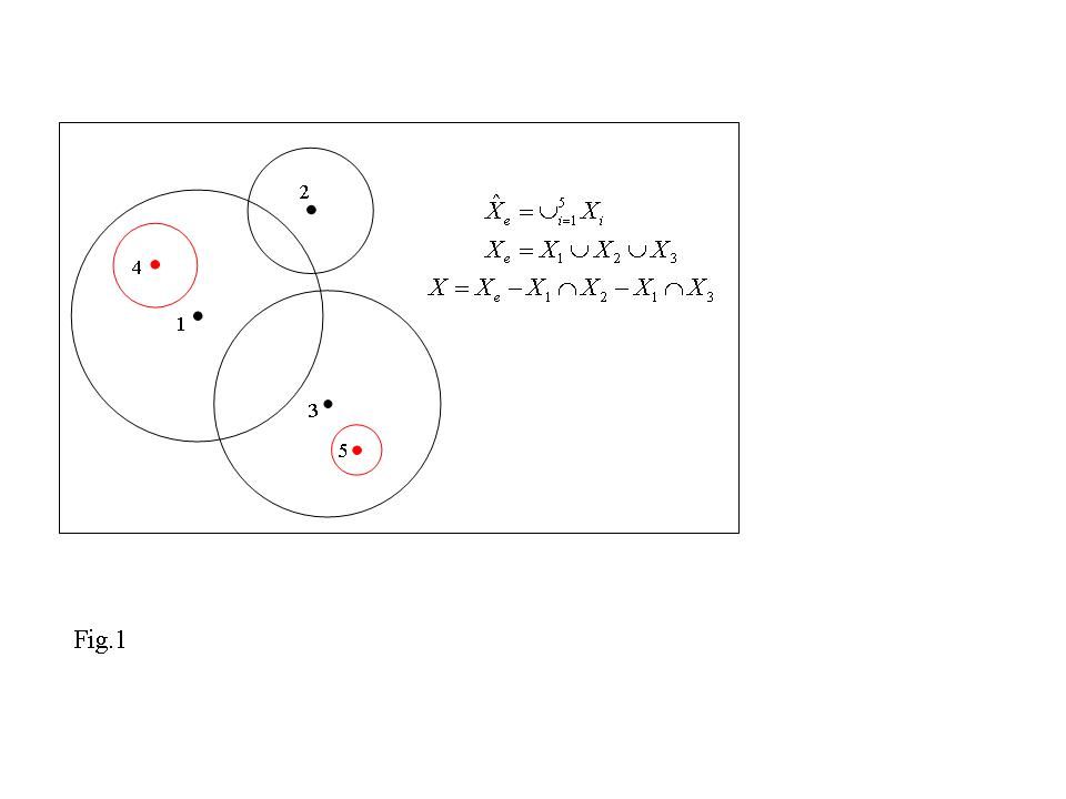
Figure 1: Pictorial view of a random ensemble of actual (dots 1-3) and phantom (dots 4-5) nuclei. The definitions of both phantom included ($\hat{X_{e}}$) and actual ($X_{e}$) extended fractions are also reported. The (extended) volume of the i-th nucleus is denoted as $X_{i}$ and the transformed fraction as $X$.

The aim of this contribution is twofold: i) to model the phase transformation kinetics in terms of actual quantities such as the nucleation rate; ii) to provide an expression for the transformed fraction as a function of $X_{e}$.

2 Theory

In this section we discuss the stochastic theory that has to be employed in order to get rid of phantoms in modeling the kinetics of phase transformations ruled by nucleation and growth. To this end, let us define the phantom included nucleation rate $I(t)$, and the ”actual” nucleation rate, $I_{a}(t)$, namely the rate of birth of the ”real” nuclei; $I_{a}(t)$ is the quantity experimentally accessible. It goes without saying that a mathematical formulation of the phase transition kinetics which employs the ”actual” nucleation rate holds true for both KJMA-compliant and KJMA-non-compliant growth laws. This automatically overcomes the limit of the KJMA approach. However, actual nuclei imply a severe complication of the stochastic-nature of the process under study, for we shift from a Poissonian to a non-Poissonian process: in fact actual nuclei are spatially correlated. Let us address this point in more detail by denoting with $R(t,t^{\prime})$ the radius of a nucleus, at running time $t$, which starts growing at time $t^{\prime}<t$. To be an actual nucleus it has to lie at a distance $r>R(t^{\prime},t^{\prime\prime})$ from any other ”older” nucleus with $t^{\prime\prime}<t^{\prime}$. In other words, in the spirit of the statistical mechanics of hard spheres, this condition is formalized (at the lowest order) through the pair distribution function for the ”pair of nuclei ($t^{\prime},t^{\prime\prime}$)” at relative distance $r$

$$f_{2}(r,t^{\prime},t^{\prime\prime})\approx H(r-R(t^{\prime},t^{\prime\prime})),$$ (1)

where $H(x)$ is the Heavyside function. Throughout the paper we employ the notation by Van Kampen [20] according to which $n-$dots distribution and correlation functions are denoted as $f_{n}$ and $g_{n}$, respectively.

In previous papers, we have presented a theory for describing phase transitions in the case of spatially correlated nuclei and for time dependent nucleation rate [21, 22]. The untransformed fraction can be expressed in terms of either the distribution functions, ($f_{n}$-functions), or the correlation functions, ($g_{n}$-functions), where the $f_{n}$’s and $g_{n}$’s are linked by cluster expansion [20]. Given a generic point of space we have computed the probability that this point is not covered (transformed) by any nucleus up to time $t$. This probability is the fraction of untransformed phase i.e. $Q(t)=1-X(t)$. By denoting with $\Delta(t,t^{\prime})$ the volume of a nucleus, which starts growing at time $t^{\prime}<t$, at running time $t$, and in the case of symmetric $f_{n}$ and $g_{n}$ functions, the uncovered fraction is given by

$$Q(t) = 1-\int_{0}^{t}\tilde{I}(t_{1})dt_{1}\int_{\Delta(t,t_{1})}f_{1}(\mathbf{r}_{1})d\mathbf{r}_{1}+$$

$$+ \int_{0}^{t}\tilde{I}(t_{1})dt_{1}\int_{0}^{t_{1}}\tilde{I}(t_{2})dt_{2}\int_{\Delta(t,t_{1})}d\mathbf{r}_{1}\int_{\Delta(t,t_{2})}d\mathbf{r}_{2}f_{2}(\mathbf{r}_{1},\mathbf{r}_{2})-....$$

$$= 1+$$

$$+ \sum_{m=1}^{\infty}\frac{(-1)^{m}}{m!}\int_{0}^{t}\tilde{I}(t_{1})dt_{1}..\int_{0}^{t}\tilde{I}(t_{m})dt_{m}\times$$

$$\>\int_{\Delta(t,t_{1})}d\mathbf{r}_{1}\int_{\Delta(t,t_{2})}d\mathbf{r}_{2}....\int_{\Delta(t,t_{m})}f_{m}(\mathbf{r}_{1},..,\mathbf{r}_{m})d\mathbf{r}_{m}$$

or,

$$Q(t) = \exp\Big{[}\sum_{m=1}^{\infty}\frac{(-1)^{m}}{m!}\int_{0}^{t}\tilde{I}(t_{1})dt_{1}...\int_{0}^{t}\tilde{I}(t_{m})dt_{m}$$ (3)

$$\>\int_{\Delta(t,t_{1})}d\mathbf{r}_{1}\int_{\Delta(t,t_{2})}d\mathbf{r}_{2}....\int_{\Delta(t,t_{m})}g_{m}(\mathbf{r}_{1},..,\mathbf{r}_{m})d\mathbf{r}_{m}\Big{]}.$$

It is worth pointing out that the nucleation rates entering these equations are in fact subjected to the condition imposed by the correlation among nuclei. This quantity may or may not imply phantoms depending on the specific form of the $f_{n}$ functions. For this reason we introduce the new symbol $\tilde{I}$. In particular, for the hard core correlation (eqn.1) $\tilde{I}$ coincides with the actual nucleation rate, $\tilde{I}=I_{a}$, which leads to the solution of the phase transition kinetics in terms of the actual nucleation rate.

Since eqn.2,3 are the exact solutions of the stochastic process linked to the phase transition, they also coincide with the KJMA formula provided the above mentioned preconditions are met i.e. random nucleation and KJMA-compliant growth.

As far as the hard-core correlation (eqn.1) and the kinetics eqns.2,3 are concerned, we note that the number of nuclei of size $R(t,t_{1})$ is $I_{a}(t_{1})dt_{1}=O(dt_{1})$. As a consequence and in the framework of the statistical mechanics of hard sphere fluid, we are dealing with an extremely dilute solution of pairs of components $"t_{1},t_{2}"$. Accordingly, the number density of $t_{2}$ spheres being of the order of $O(dt_{2})$, higher order terms in the cluster expansion of the $f_{2}$ function can be neglected, thus $f_{2}(r,t^{\prime},t^{\prime\prime})=H(r-R(t^{\prime},t^{\prime\prime}))$ in eqn.2.

2.1 KJMA-compliant growths

In this section we show that eqn.2 is compatible with the KJMA kinetics only in the case of KJMA-compliant function. On the other hand, such a comparison will give a deeper insight into the reasons why the KJMA kinetics does not work in the case of ”KJMA-non-compliant” functions. In the following, we discuss the linear growth law for 2D case. Also, to simplify the complexity of the computation the ”actual” nucleation rate, $I_{a}$, is taken as constant; as a consequence the phantom included nucleation rate reads [3, 19] $I(t)=I_{a}/(1-X(t))=I_{a}/Q(t)\equiv I_{a}F(t)$ and the KJMA kinetics becomes

$$F(t)=\exp\Big{[}\int_{0}^{t}I_{a}F(t^{\prime})\pi R^{2}(t,t^{\prime})dt^{\prime}\Big{]},$$ (4)

where $R(t,t^{\prime})=v(t-t^{\prime})$ and $v$ is a constant.

We consider the series expansion of $F(t)$ around $t=0$. One gets,

$$\frac{d^{n+1}F(t)}{dt^{n+1}}\equiv F^{(n+1)}=(F\Omega)^{(n)}=\sum_{k=0}^{n}(^{n}_{k})F^{(n)}\Omega^{(n-k)},$$ (5)

where $\Omega(t)=2\pi I_{a}\int_{0}^{t}F(t^{\prime})R(t,t^{\prime})\partial_{t}R(t,t^{\prime})dt^{\prime}=2\pi I_{a}v\int_{0}^{t}F(t^{\prime})R(t,t^{\prime})dt^{\prime}$.

Moreover, since $\Omega^{(m+2)}=\kappa F^{(m)}$, being $\kappa=2\pi v^{2}I_{a}$ and $F^{(0)}=1,\Omega^{(0)}=\Omega^{(1)}=0$, from eqn.5 it is found that only the terms $F^{(3n)}(0)$ are different from zero, i.e. $F(t)=\sum_{n=0}^{\infty}\frac{1}{(3n)!}F^{(3n)}(0)t^{3n}=\sum_{m=0}^{\infty}c_{m}t^{m}$. In particular, the first coefficients are: $F^{(3)}(0)=\kappa,F^{(6)}(0)=11\kappa^{2},F^{(9)}(0)=375\kappa^{3},F^{(12)}(0)=234147\kappa^{4}$.

Next we derive the series expansion of the untransformed fraction $Q(t)=\sum_{n=0}^{\infty}b_{n}t^{n}$, by exploiting the condition $1=Q(t)F(t)=\sum_{n=0}^{\infty}b_{n}t^{n}\sum_{m=0}^{\infty}c_{m}t^{m}$. Even in this case the $b_{n}$ coefficients are different from zero for $n=3k$ (with integer $k$). The first four coefficients are

$$\begin{array}[]{l}b_{0}=\frac{1}{c_{0}}=1\\ b_{3}=-c_{3}\\ b_{6}=-c_{6}+c_{3}^{2}\\ b_{9}=-c_{9}+2c_{3}c_{6}-c_{3}^{2}.\end{array}$$ (6)

By using the expression of $c_{n}$’s the series of the untransformed fraction up to $t^{9}$ is given as

$$\begin{array}[]{l}Q(t)=1-\frac{1}{6}\kappa t^{3}+\frac{1}{80}\kappa^{2}t^{6}-\frac{207}{9!}\kappa^{3}t^{9}+O(t^{12}).\end{array}$$ (7)

Since $X_{e}=\frac{1}{3!}\kappa t^{3}=\frac{1}{3}\pi I_{a}v^{2}t^{3}=\int_{0}^{t}I_{a}\pi R^{2}(t,t^{\prime})dt^{\prime}$ the series eqn.7 can be rewritten as

$$Q(t)=1-X_{e}+\frac{9}{20}X_{e}^{2}-\frac{69}{560}X_{e}^{3}+O(X_{e}^{4}),$$ (8)

the two last coefficients being $0.45$ and $0.123$. We emphasize that the coefficients of this series only depend upon growth law, for constant $I_{a}$ (see also the last section).

The next step is to show that the untransformed fraction, given by the series eqn.2 is equal to eqn.7 or eqn.8. We have carried out the first two terms, exactly, while, owing to the tremendous computational complexity, for the third term an approximation has been employed. It is worth reminding that the distribution functions are $f_{1}(\mathbf{r}_{1})=1,f_{2}(\mathbf{r}_{12},t_{1},t_{2})=H(r_{12}-R(t_{1},t_{2}))$ and $f_{3}(\mathbf{r}_{12},\mathbf{r}_{13},\mathbf{r}_{23},t_{1},t_{2},t_{3})=H(r_{12}-R(t_{1},t_{2}))H(r_{13}-R(t_{1},t_{3}))H(r_{23}-R(t_{2},t_{3}))$, where $\mathbf{r}_{ij}$ is the relative distance. In fact, since $I_{a}dt_{i}=O(dt_{i})$ the system of dots is dilute and $f_{3}(1,2,3)=f_{2}(1,2)f_{2}(1,3)f_{2}(3,2)$ i.e. the superposition principle holds true [23]. Since the system is homogeneous the $f_{n}$ functions depend on $r_{ij}=|\mathbf{r}_{ij}|=|\mathbf{r}_{i}-\mathbf{r}_{j}|$. Eqn.2 becomes

$$\begin{array}[]{c}Q(t)=1-I_{a}\int_{0}^{t}dt_{1}\int_{\Delta(t,t_{1})}d\mathbf{r}_{1}+\\ \\ +I_{a}^{2}\int_{0}^{t}dt_{1}\int_{0}^{t_{1}}dt_{2}\int_{\Delta(t,t_{1})}d\mathbf{r}_{1}\int_{\Delta(t,t_{2})}d\mathbf{r}_{2}H(r_{12}-R(t_{1},t_{2}))+\\ \\ -I_{a}^{3}\int_{0}^{t}dt_{1}\int_{0}^{t_{1}}dt_{2}\int_{0}^{t_{2}}dt_{3}\int_{\Delta(t,t_{1})}d\mathbf{r}_{1}\int_{\Delta(t,t_{2})}d\mathbf{r}_{2}\times\\ \\ \int_{\Delta(t,t_{3})}d\mathbf{r}_{3}H(r_{12}-R(t_{1},t_{2}))H(r_{23}-R(t_{2},t_{3}))H(r_{13}-R(t_{1},t_{3}))+...,\end{array}$$ (9)

where the integration domain $\Delta(t,t_{i})$ is the circle of radius $R(t,t_{i})=v(t-t_{i})$. The $f_{1}$ containing term is the extended surface fraction $X_{e}(t)=I_{a}\int_{0}^{t}dt_{1}|\Delta(t,t_{1})|$ and coincides with the second term of the expansion eqn.8. Let us focus our attention on the integrals in the spatial domain - for the sake of clarity shown in fig.2a together with the circle of correlation $R(t_{1},t_{2})$- of the $f_{2}$ containing term. By employing relative coordinates the integrals read

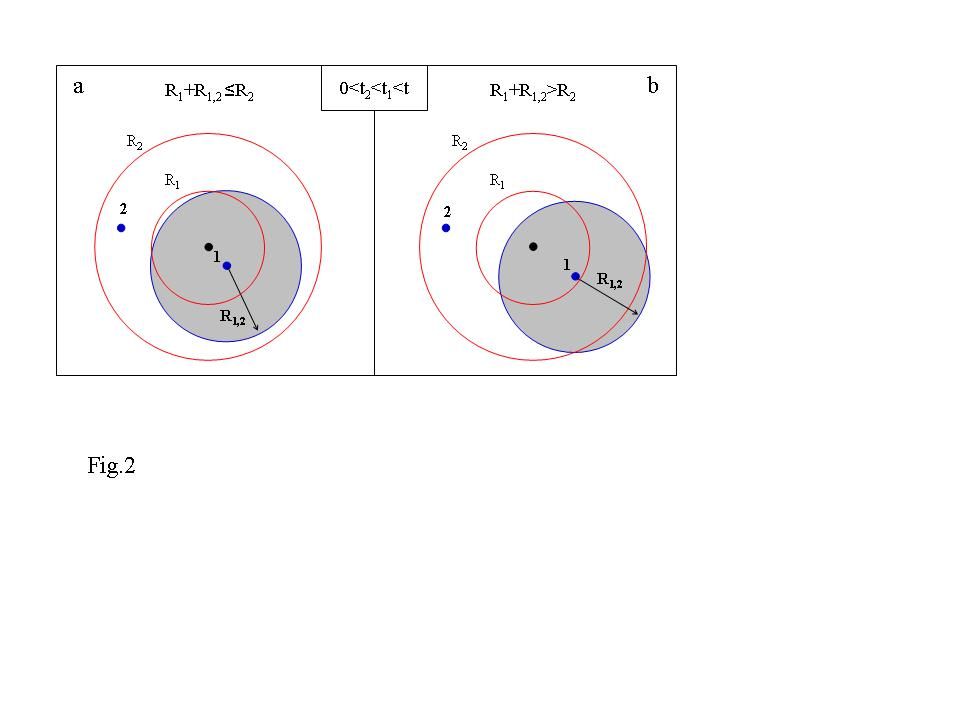
Figure 2: The integration domains and the correlation circles are depicted for the integrals over the $f_{2}$ function. The cases of KJMA-compliant and KJMA-non-compliant growths are reported in panels a and b, respectively. In the drawing $R_{12}\equiv R(t_{1},t_{2})$, $R_{i}\equiv R(t,t_{i})$ ($i=1,2$) and $t_{2}<t_{1}$. In the case of KJMA-compliant growth $R_{1}+R_{12}\leq R_{2}$ and the hard core circle is within the integration domain, $R_{2}$ (a). In the case of KJMA-non-compliant growths $R_{1}+R_{12}>R_{2}$ and the hard core disk overcomes the integration domain of the ”older nucleus” (b).

$$\int_{\Delta(t,t_{1})}d\mathbf{r}_{1}\int_{\Delta(t,t_{2})}d\mathbf{r}_{12}H(r_{12}-R(t_{1},t_{2}))=\int_{\Delta(t,t_{1})}d\mathbf{r}_{1}A(r_{1},t,t_{1},t_{2}),$$ (10)

where $A(r_{1},t,t_{1},t_{2})=A(r_{1},R(t,t_{2}),R(t_{1},t_{2}))$ is the area ”spanned” by the second nucleus when the first one is located at $\mathbf{r}_{1}$ ($t_{2}<t_{1}<t$). It is at this point of the computation that the growth law comes into play; indeed in the case of KJMA-compliant growth laws (here linear growth) the correlation circle $R(t_{1},t_{2})$ is entirely within the integration domain $R(t,t_{2})$ (fig.2a). Consequently,

$$A(t,t_{1},t_{2})=\pi\big{[}R^{2}(t,t_{2})-R^{2}(t_{1},t_{2})\big{]}$$ (11)

is independent of $\mathbf{r}_{1}$. On the other hand, in the case of KJMA-non-compliant growth laws the correlation circle overcomes the integration domain of the second nucleus and the relationship above does not hold true, anymore (see fig.2b). In general, the KJMA-compliant functions satisfy the condition $R(t,t_{1})+R(t_{1},t_{2})\leq R(t,t_{2})$ i.e. for a power growth law $(t-t_{1})^{n}+(t_{1}-t_{2})^{n}\leq(t-t_{2})^{n}$, which is verified only for $n\geq 1$. In fact, by setting $\tau=t_{1}-t_{2}$ and $\eta=\frac{t-t_{2}}{\tau}>1$, the inequality above reads $(\eta-1)^{n}\leq\eta^{n}-1$, which is satisfied for $n\geq 1$. On the other hand, for $n=1/k$ (with integer $k>1$) the inequality is $[(\eta-1)^{1/k}+1]^{k}\leq\eta$ namely,

$$\sum_{\mu=1}^{k-1}(^{k}_{\mu})(\eta-1)^{\frac{\mu}{k}}\leq 0,$$ (12)

which is never satisfied ($\eta>1$).

For the KJMA-compliant growth the contribution of the $f_{2}$ containing term becomes

$$\begin{array}[]{c}\pi I_{a}^{2}\int_{0}^{t}dt_{1}\int_{0}^{t_{1}}dt_{2}\int_{\Delta(t,t_{1})}d\mathbf{r}_{1}\big{[}R^{2}(t,t_{2})-R^{2}(t_{1},t_{2})\big{]}\\ \\ =\pi^{2}I_{a}^{2}\int_{0}^{t}dt_{1}\int_{0}^{t_{1}}dt_{2}R^{2}(t,t_{1})\big{[}R^{2}(t,t_{2})-R^{2}(t_{1},t_{2})\big{]}\\ \\ =\frac{X_{e}^{2}}{2}-\pi^{2}I_{a}^{2}\int_{0}^{t}dt_{1}\int_{0}^{t_{1}}dt_{2}R^{2}(t,t_{1})R^{2}(t_{1},t_{2}).\end{array}$$ (13)

It is possible to show that for linear growth the last term of eqn.13 is equal to $\frac{1}{180}(\pi I_{a}v^{2}t^{3})^{2}$, consequently we get $\frac{X_{e}^{2}}{2}-\frac{9X_{e}^{2}}{180}=\frac{9}{20}X_{e}^{2}$, which coincides with the term of the same order in the KJMA series eqn.8.

Let’s now briefly consider the contribution of the $f_{3}$ containing term in the general expression eqn.2. Fig.3 shows the integration domains $R_{i}=R(t,t_{i})$ and the correlation circles $R(t_{i},t_{j})$ for the three nuclei born at time $t_{i}$ ($i=1,2,3$). The configuration integral over $f_{3}$ in eqn.9 becomes

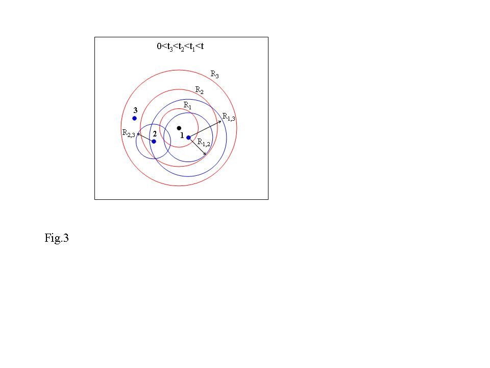
Figure 3: Integration domains and correlation hard disks for the integral over the $f_{3}$ function. In the drawing $R_{ij}\equiv R(t_{i},t_{j})$ and $R_{i}\equiv R(t,t_{i})$. In the case of KJMA-compliant growth all the circles are entirely within the $R(t,t_{3})$ circle.

$$\begin{array}[]{l}I_{a}^{3}\int_{0}^{t}dt_{1}\int_{0}^{t_{1}}dt_{2}\int_{0}^{t_{2}}dt_{3}\int_{\Delta(t,t_{1})}d\mathbf{r}_{1}\int_{\Delta(t,t_{2})}d\mathbf{r}_{2}H(r_{12}-R(t_{1},t_{2}))\times\\ \\ \int_{\Delta(t,t_{3})}d\mathbf{r}_{3}H(r_{13}-R(t_{1},t_{3}))H(r_{23}-R(t_{2},t_{3}))\\ \\ =I_{a}^{3}\int_{0}^{t}dt_{1}\int_{0}^{t_{1}}dt_{2}\int_{0}^{t_{2}}dt_{3}\times\\ \\ \int_{\Delta(t,t_{1})}d\mathbf{r}_{1}\int_{\Delta(t,t_{2})}d\mathbf{r}_{2}H(r_{12}-R(t_{1},t_{2}))A(r_{12},R(t_{1},t_{3}),R(t_{2},t_{3})),\end{array}$$ (14)

where $t_{3}<t_{2}<t_{1}<t$ is assumed. In this equation, $A(r_{12},R(t_{1},t_{3}),R(t_{2},t_{3}))$ is the area spanned by the third nucleus when the first and the second are located at $\mathbf{r}_{1}$ and $\mathbf{r}_{2}$, respectively. Because of the possible overlap between the correlation circles $R(t_{1},t_{3})$ and $R(t_{2},t_{3})$, and for $R(t_{1},t_{3})$ is encompassed within $R(t,t_{3})$ this area is a function of $r_{12}$ as

$$\begin{array}[]{l}A(r_{12})=\omega(r_{12})H(R(t_{1},t_{3})+R(t_{2},t_{3})-r_{12})+\\ \\ +\pi\big{[}R^{2}(t,t_{3})-R^{2}(t_{1},t_{3})-R^{2}(t_{2},t_{3})\big{]}H(r_{12}-R(t_{2},t_{3})-R(t_{1},t_{3})),\end{array}$$ (15)

where $\omega(r_{12})=\pi(R^{2}(t,t_{3})-R^{2}(t_{1},t_{3})-R^{2}(t_{2},t_{3}))+\varpi(r_{12},R(t_{1},t_{3}),R(t_{2},t_{3}))$, with $\varpi(x,\rho_{1},\rho_{2})$ being the overlap area of two circles of radius $\rho_{1}$ and $\rho_{2}$ at relative distance $x$

$$\begin{array}[]{l}\varpi(x,\rho_{1},\rho_{2})=-\frac{1}{2}\sqrt{4x^{2}\rho_{1}^{2}-[\rho_{2}^{2}-x^{2}-\rho_{1}^{2}]^{2}}+\\ \\ +\rho_{1}^{2}\arccos\frac{\rho_{1}^{2}+x^{2}-\rho_{2}^{2}}{2x\rho_{1}}+\rho_{2}^{2}\arccos\frac{\rho_{2}^{2}+x^{2}-\rho_{1}^{2}}{2x\rho_{2}}.\end{array}$$ (16)

It turns out that the computation of the third order term of the series, eqn.14, is a formidable task indeed. We do not attempt to perform the exact estimate of this term which, however, must coincide with the same order term of the KJMA series. On the other hand, an approximate evaluation of this term by using an oversimplified form of the $A(r_{12})$ area, is possible by formally rewriting this area as $A(r_{12})=\pi[R^{2}(t,t_{3})-R^{2}(t_{1},t_{3})-\beta R^{2}(t_{2},t_{3})]$, where $\beta\in(0,1)$ is given by $\beta=[1-\frac{\varpi(r_{12})}{\pi R^{2}(t_{2},t_{3})}H(R(t_{1},t_{3})+R(t_{2},t_{3})-r_{12})]$. In the case of complete-overlap ($\beta=0$) we get,

$$\begin{array}[]{l}\pi^{3}I_{a}^{3}\int_{0}^{t}dt_{1}\int_{0}^{t_{1}}dt_{2}\int_{0}^{t_{2}}dt_{3}R^{2}(t,t_{1})[R^{2}(t,t_{2})-R^{2}(t_{1},t_{2})][R^{2}(t,t_{3})-R^{2}(t_{1},t_{3})],\par\end{array}$$ (17)

that for the linear growth ($R(t,t^{\prime})=v(t-t^{\prime})$) gives $\frac{24}{7!}I_{a}^{3}\pi^{3}v^{6}t^{9}=\frac{72}{560}X_{e}^{3}$ to be compared with the exact value $\frac{69}{560}X_{e}^{3}$ which brings an uncertainty of $4.3\%$ .

2.2 KJMA-non-compliant growths

Let us now consider the parabolic growth $R(t,t^{\prime})=v\sqrt{t-t^{\prime}}$. In this case the series expansion of the function $F(t)=1/Q(t)$, given by eqn.4, can be performed by employing the same computation pathway discussed above, where now $\Omega^{(n+1)}=\kappa F^{(n)}$ and $\kappa=\pi I_{a}v^{2}$. In this case $F^{(2n)}(0)\neq 0$ implying $F(t)=1+\frac{\kappa}{2}t^{2}+\frac{1}{6}\kappa^{2}t^{4}+\frac{34}{6!}\kappa^{3}t^{6}$ and

$$\begin{array}[]{c}Q(t)=1-\frac{\kappa}{2}t^{2}+\frac{\kappa^{2}}{12}t^{4}-\frac{\kappa^{3}}{180}t^{6}+O(t^{8})\\ \\ =1-X_{e}+\frac{1}{3}X_{e}^{2}-\frac{4}{90}X_{e}^{3}+O(X_{e}^{4}),\end{array}$$ (18)

the two last coefficients being $0.33$ and $0.044$. It is worth pointing out that in such an evaluation the transformed fraction, $X$, is comprehensive of the contribution of phantoms. In fact, we recall that eqn.4 is the KJMA solution with the phantom included nucleation rate, $I_{a}/(1-X)$.

The $f_{1}$ containing term of eqn.2 gives the extended volume fraction $\frac{\kappa}{2}t^{2}$. As far as the third term is concerned ($f_{2}$ contribution), it is possible to show that also for $n=1/2$ the integral eqn.13 coincides with the third term of eqn.18, $\frac{\kappa^{2}}{12}t^{4}$. However, it is important to stress that eqn.13 does not coincide, in this case, with the integral over the $f_{2}$ function of the exact solution eqn.9, since in the latter equation enter the actual nuclei, only. From the mathematical point of view, in the case of parabolic growth, the correlation circle is not contained within the integration domain as depicted in Fig.2b. In other words, for KJMA-non-compliant growth laws the area $A$ is a function of $r_{1}$ and the term of order $I_{a}^{2}$ in eqn.9 does not coincide with $\frac{X_{e}^{2}}{3}$ of eqn.18 (parabolic growth). In particular, under these circumstances we get

$$\begin{array}[]{c}A(r_{1},t,t_{1},t_{2})=\omega(r_{1})H(r_{1}+R(t_{1},t_{2})-R(t,t_{2}))+\\ \\ +\pi\big{[}R^{2}(t,t_{2})-R^{2}(t_{1},t_{2})\big{]}H(R(t,t_{2})-r_{1}-R(t_{1},t_{2})),\end{array}$$ (19)

where $\omega(r_{1})=\pi R^{2}(t,t_{2})-\varpi(r_{1},R(t,t_{2}),R(t_{1},t_{2}))$ with $\varpi(r_{1})$ the overlap area of two circles of radius $R(t,t_{2})$ and $R(t_{1},t_{2})$ at distance $r_{1}$ (eqn.16).

3 Numerical Simulations

The ultimate aim of this section is to propose a simple formula for describing the kinetics on the basis of the ”actual” extended transformed fraction, $X_{e}$. On the ground of eqn.3 the transformed fraction can be rewritten in the general form

$$X(t)=1-\exp[-X_{e}(t)\gamma(X_{e}(t))],$$ (20)

where $\gamma(X_{e}(t))$ embodies the contributions of correlations among nuclei [21]. It is worth noticing that for KJMA-complaint growths (random nucleation) eqn.3 actually reproduces the KJMA formula. In fact by identifying $\tilde{I}$ with the phantom included nucleation rate ( $\tilde{I}\equiv I$) one gets $g_{m>1}=0$ leading to the formula $Q=\exp(-\hat{X_{e}})$. On the other hand, working with the actual nucleation rate, in eqn.3 $\tilde{I}\equiv I_{a}$, $g_{m}\neq 0$ and the series has infinite terms. $\gamma(X_{e}(t))$ can therefore be expanded as a power series of the extended actual volume fraction, $X_{e}$. Moreover, by exploiting the homogeneity properties of the $f_{n}$ functions (see below), it is possible to attach a physical meaning to the power series coefficients, in terms of nucleation rate and growth law. Also, for constant $I_{a}$ the coefficients of this series only depend upon growth law. To the aim of achieving a suitable compromise between handiness and pliability, we retain the liner approximation of $\gamma(X_{e}(t))$ obtaining the following kinetics

$$X=1-\exp[-(aX_{e}+bX_{e}^{2})],$$ (21)

with $a$ and $b$ constants. For the sake of completeness we point out that, according to its physical meaning, the parameter $a$ should be unitary. Nevertheless, the substitution of the infinite expansion with only two terms authorizes the introduction of the new parameter $a$. In any case, the $a$ values are found to be nearly one (see fig.7 below).

In order to study the transition kinetics in terms of actual nuclei and to test eqn.21, we worked out 2D computer simulations for several growth laws at constant nucleation rate, $I_{a}$.

As typical for this kind of study [5], [24], the simulation is performed on a lattice (square in our case) where, in order to mimic the continuum case, the lattice space is much lower than the mean size of nuclei.

In particular, the transformation takes place on a square lattice whose dimension is $1000\times 1000$ with a nucleation rate of $I_{a}=3$. It is worth reminding that, since the nucleation is Poissonian, it occurs on the entire lattice independently of whether the space is already transformed or not. The computer simulation can be run taking into account the presence of phantoms or not. In the former case the outputs have been labeled as ”w” while the latter as ”wo”. As far as the growth laws are concerned, we limited ourself to the power laws, $R(t)\sim t^{n}$ for $n=1/4,1/3,1/2,1,3/2$ and $2$.

The results of the simulations are displayed in figs.4a-c for the KJMA-non-compliant growths. In particular, the fractional surface coverage,$X$, as a function of the actual extended fraction $X_{e}$, with and without the contribution of phantoms, are reported (curves labeled with ”w” and ”wo”, respectively).

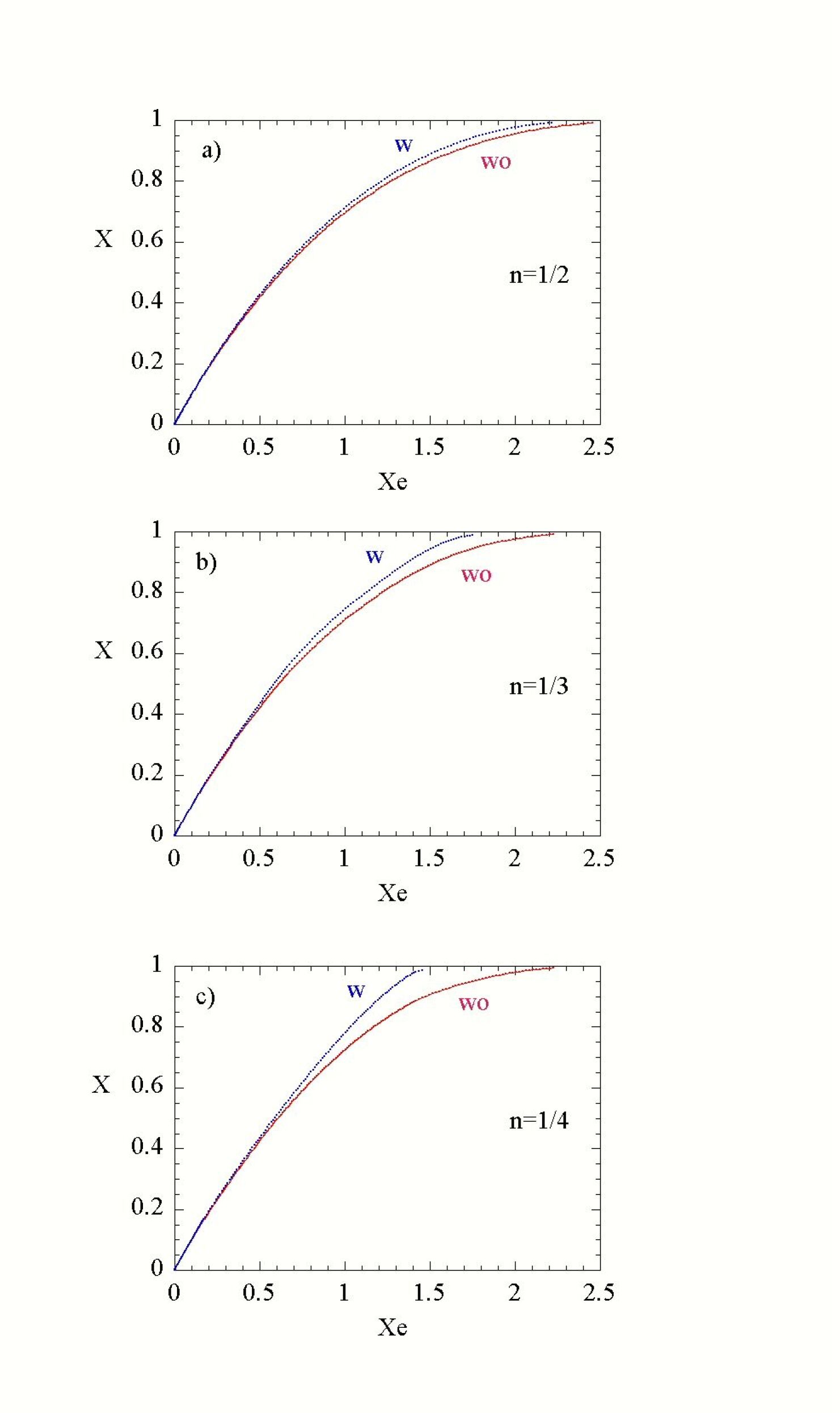
Figure 4: Computer simulatiosn of phase transformations ruled by KJMA-non-compliant growths. The surface fraction, $X$, is shown as a function of the extended fraction $X_{e}$, for the power law ($R\approx t^{n}$) where $n=1/2$, $1/3$ and $1/4$ in figures a, b and c, respectively. The kinetics with (w) and without (wo) the inclusion of phantoms are displayed.

The contribution of phantom overgrowth to the transformation kinetics is highlighted in fig.5 and shows that this effect brings an uncertainty on $X$ which ranges from $2\%$ to $5\%$ on going from $n=1/2$ to $n=1/4$. In the case of parabolic growth this figure is lower than $2\%$.

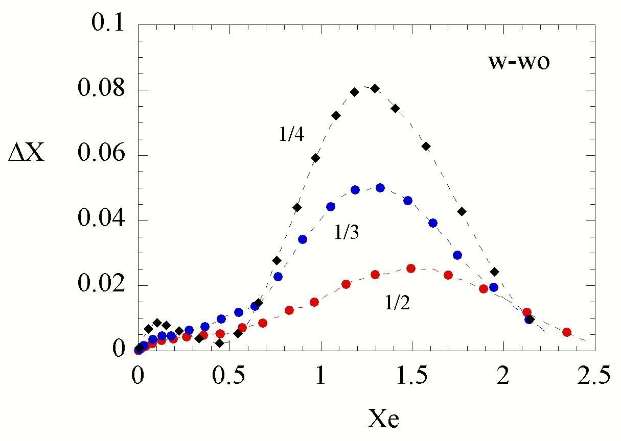
Figure 5: Contribution of phantom overgrowth to the kinetics reported in fig.4 (displayed is the difference between curves (w) and (wo)). The area beneath the curves normalized to the area of the kinetics of fig.4 are, respectively, $0.053$, $0.038$ and $0.02$ for $n=1/4$, $n=1/3$ and $n=1/2$.

These results are in qualitative agreement with previous studies on phantom overgrowth, although performed for a different nucleation laws [24, 16]. As discussed in more details below, the results displayed in figs.4,5 are universal, i.e. they only depend on power exponent, $n$, and nucleation law (in the present case $I_{a}=constant$). Accordingly, the lower $n$ the more important is phantom overgrowth. In fact, let us consider a phantom, which starts growing at time $\bar{t}$, located at $r_{p}$ from the center of an actual nucleus which starts growing at $t=0$ (fig.6a). For KJMA-non-compliant growth, $R(t-t^{\prime})=v(t-t^{\prime})^{\frac{1}{k}}$ (with integer $k>1$), the phantom overtakes the actual nucleus at time $t_{o}$, that is the solution of the equation $r_{p}+v(t_{o}-\bar{t})^{\frac{1}{k}}=vt_{o}^{\frac{1}{k}}$, namely

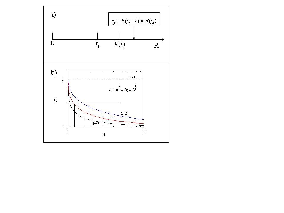
Figure 6: Sketch of the overgrowth process in the space domain. $r_{p}$ denotes the location of the phantom which start growing at time $\bar{t}$ when the size of the actual nucleus is $R(\bar{t})$. The phantom overtakes the actual nucleus at time $t_{o}$ when the size of the actual nucleus is $R(t_{o})$.

$$\xi=\eta^{\frac{1}{k}}-(\eta-1)^{\frac{1}{k}},$$ (22)

where $\xi=\frac{r_{p}}{v\bar{t}^{\frac{1}{k}}}<1$ and $\eta=\frac{t_{o}}{\bar{t}}>1$. The graphical solution of eqn.22 is depicted in fig.6b and indicates that $t_{o}$ (and therefore $\eta$) decreases with $k$. This is in agreement with the results of fig.5 which shows that the overgrowth phenomenon is more important at greater $k$.

As far as the guess function eqn.21 is concerned, it matches the simulation curves with a very high degree of correlation. For instance the output of the fit to the $n=2$ curve, gives $a=0.9750\pm 0.0007$, $b=0.088\pm 0.001$ and a squared correlation coefficients practically $1$. For the sake of completeness the $a$ and $b$ fitting parameters are shown in fig.7, where $a$ is found to be nearly one. This is in agreement with the theoretical value predicted by eqn.3.

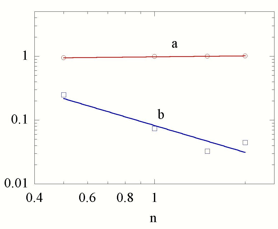
Figure 7: Behavior of the fitting parameters a and b of eqn.21 as a function of growth exponent $n$, for KJMA-non-compliant growths.

The behavior of the transformed fraction for KJMA-compliant growths are reported in fig.8 for $n=1$, $n=3/2$ and $n=2$.

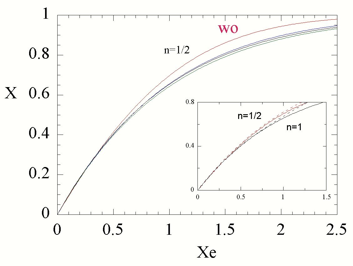
Figure 8: Kinetics of the actual surface fraction, as a function of actual extended surface fraction, for several values of $n$. In the graph the kinetics for $n=1/2$ is compared with the KJMA-compliant growth with $n=1$, $n=2$ and $n=3/2$ (from the top, respectively). In the inset the kinetics for $n=1$ and $n=1/2$ are displayed together with the truncated KJMA series expansions eqn.8 and eqn.18, respectively.

These kinetics are very close to each other and differs, markedly, from that at $n=1/2$ also reported in the same figure. In the inset, the kinetics for $n=1/2$ and $n=1$ are compared with the KJMA series expansion eqn.18 and eqn.8, respectively. The fact that the curves for $n=1$, $3/2$ and $2$ collapse on the same curve, can be rationalized computing the coefficients of the series expansion of $Q(X_{e})$ for integer $n$. In particular, by employing the method discussed in the previous section the two last coefficients of the series (e.g. eqn.8) are $0.4960$, $0.1633$ and $0.5$, $0.1673$ for $n=2$ and $3$, respectively. We also performed computer simulations of phase transitions for non-constant actual nucleation rate. The output of this computation is displayed in fig.9 where the behavior of the nucleation rate is shown in the inset as function of $X_{e}$. In particular, the actual nucleation rate is given by the function $I_{a}(t)\approx t^{2}\exp(-\tilde{a}t^{3})$.

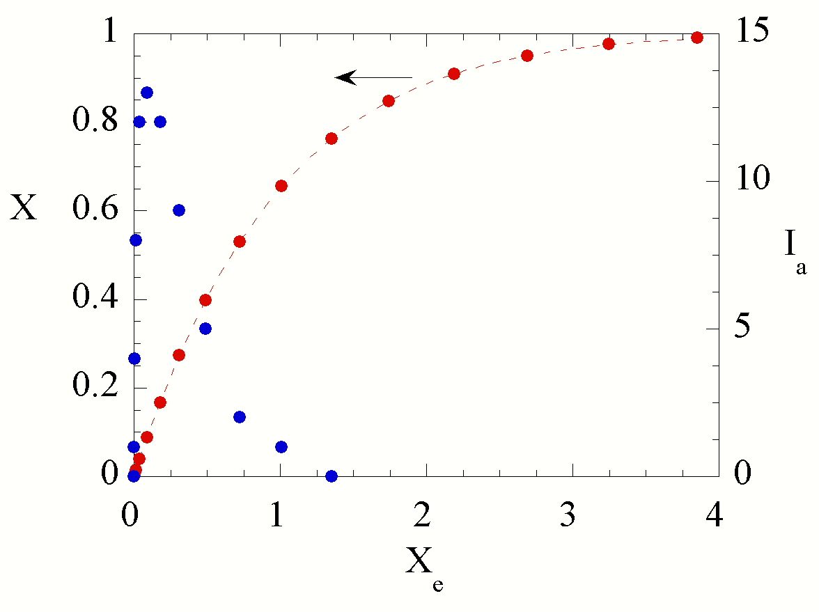
Figure 9: Fig.9 Kinetics of the actual surface fraction, as a function of the actual extended surface, for non-constant actual nucleation rate (left scale). The best fit of the function eqn.21 to the $X(X_{e})$ kinetics has been shown as dashed line. The correlation coefficient of the fit is in fact $1$ for the parameters $a=1.014$ and $b=0.0382$. The actual nucleation rate, as a function of $X_{e}$, is also reported on the right scale in $nuclei\times 10^{6}/site$ units.

Also in this case the function eqn.21 has been found to match the kinetics with high degree of correlation where, again, the independent variable is the actual extended surface fraction.

Let us address in more detail the question of the dependence of volume fraction on extended volume fraction. To this end, we discuss the second order term of the exact solution eqn.2, namely

$$\int_{0}^{t}I_{a}(t^{\prime})dt^{\prime}\int_{0}^{t^{\prime}}I_{a}(t^{\prime\prime})dt^{\prime\prime}\int_{\Delta(t,t^{\prime})}d\mathbf{r}_{1}A(r_{1},R(t^{\prime},t^{\prime\prime}),R(t,t^{\prime\prime})),$$ (23)

where eqn.10 has been employed. We point out that in eqn.23 $A(r_{1},R(t^{\prime},t^{\prime\prime}),R(t,t^{\prime\prime}))$ is a second order homogeneous function of $r_{1}$, $R(t^{\prime},t^{\prime\prime})$ and $R(t,t^{\prime\prime})$ variables. Accordingly, for the growth law $R(t,t^{\prime})=v(t-t^{\prime})^{n}$, using the re-scaled variables, $r^{\prime}_{1}=r_{1}/vt^{n}$, $\tau^{\prime}=t^{\prime}/t$ and $\tau^{\prime\prime}=t^{\prime\prime}/t$ the integral becomes

$$\pi^{2}v^{4}t^{4n+2}\int_{0}^{1}I_{a}(\tau^{\prime})d\tau^{\prime}\int_{0}^{\tau^{\prime}}I_{a}(\tau^{\prime\prime})d\tau^{\prime\prime}\int_{\Delta(\tau^{\prime})}d\mathbf{r}^{\prime}_{1}A(r^{\prime}_{1},\tau^{\prime},\tau^{\prime\prime}).$$ (24)

Eqn.24 takes the form $C_{2}X_{e}^{2}$ where
$C_{2}(n,[I_{a}(\tau)])=\frac{\int_{0}^{1}d\tau^{\prime}I_{a}(\tau^{\prime})\int_{0}^{\tau^{\prime}}I_{a}(\tau^{\prime\prime})d\tau^{\prime\prime}\int_{\Delta(\tau^{\prime})}A(r_{1}^{\prime},\tau^{\prime},\tau^{\prime\prime})d\mathbf{r}^{\prime}_{1}}{(\int_{0}^{1}I_{a}(\tau^{\prime})(1-\tau^{\prime})^{2n}d\tau^{\prime})^{2}}$ depends on $n$ and actual nucleation rate. It is apparent that in the case discussed in the previous section $I_{a}(t)=I_{a}$, $C_{2}(n)$, as well as higher order coefficients, is a function of $n$, only. In this case the transformed fraction is expected of the form $1-X=\sum_{k}C_{k}(n)X_{e}^{k}$.

On the other hand, in the case of a constant ”phantom-included” nucleation rate, $I_{a}(t)=I_{0}(1-X(t))=I_{0}Q(t)$, and eqn.2 becomes an integral equation for the $Q(t)$ unknown. With reference to the second order term, in this case eqn.24 takes the general form $C^{\prime}(n)\hat{X}_{e}^{2}$ which now implies the series $1-X=\sum_{k}C^{\prime}_{k}(n)\hat{X}_{e}^{k}$ (note that this is a series expansion in terms of phantom-included extended surface). In the specific case of KJMA-compliant growths, however, these series reduces to the exponential series with constant coefficients $\frac{(-1)^{k}}{k!}$. It is instructive to estimate the first two coefficients in the case of linear growth. For constant phantom included nucleation rate the untransformed fraction satisfies the integral equation,

$$\begin{array}[]{l}Q(t)=1-I_{0}\int_{0}^{t}Q(t^{\prime})|\Delta(t,t^{\prime})|dt^{\prime}+\\ \\ +I_{0}^{2}\int_{0}^{t}dt^{\prime}\int_{0}^{t^{\prime}}dt^{\prime\prime}Q(t^{\prime})Q(t^{\prime\prime})\int_{\Delta(t,t^{\prime})}d\mathbf{r}_{1}A(r_{1},t,t^{\prime},t^{\prime\prime})+O(I_{0}^{3}).\end{array}$$ (25)

The first order term of this equation, namely of the order of $I_{0}$, gives $Q(t)=1-I_{0}\pi v^{2}t^{3}/3=1-\hat{X}_{e}$. By substituting $Q\approx 1-\hat{X}_{e}$ in eqn.25, we get

$$\begin{array}[]{l}Q(t)=1-\hat{X}_{e}+I_{0}\int_{0}^{t}\hat{X}_{e}(t^{\prime})|\Delta(t,t^{\prime})|dt^{\prime}+\\ \\ +I_{0}^{2}\int_{0}^{t}dt^{\prime}\int_{0}^{t^{\prime}}dt^{\prime\prime}\int_{\Delta(t,t^{\prime})}d\mathbf{r}_{1}A(r_{1},t,t^{\prime},t^{\prime\prime})+O(I_{0}^{3}).\end{array}$$ (26)

Using dimensionless variables $r_{1}^{\prime}=r_{1}/vt$, $\tau^{\prime}=t^{\prime}/t$ and $\tau^{\prime\prime}=t^{\prime\prime}/t$ eqn.26 eventually becomes

$$\begin{array}[]{l}Q(t)=1-\hat{X}_{e}+3\hat{X}_{e}^{2}\int_{0}^{1}\tau^{\prime 3}(1-\tau^{\prime})^{2}d\tau^{\prime}+\\ \\ +9\hat{X}_{e}^{2}\int_{0}^{1}d\tau^{\prime}\int_{0}^{\tau^{\prime}}d\tau^{\prime\prime}(1-\tau^{\prime})^{2}A(\tau^{\prime},\tau^{\prime\prime})+O(I_{0}^{3}),\end{array}$$ (27)

where $A(\tau^{\prime},\tau^{\prime\prime})$ is given through eqn.11. Notably, the last term in eqn.27 has been already estimated in eqn.13 and is equal to $\frac{9}{20}\hat{X}_{e}^{2}$. The coefficient of $\hat{X}_{e}^{2}$ is eventually computed as $\frac{3}{60}+\frac{9}{20}=\frac{1}{2}$, that is the expected result.

It is worth noting that the present approach can also be applied to different convex shapes other than circles and spheres, provided the orientation of nuclei is the same (with a possible exception for triangle) . This aspect has been discussed in details in refs.[25],[26].

We conclude this section by quoting the recent results of ref.[17]. In this noteworthy contribution the author faced the problem of describing the kinetics in terms of the actual nucleation rate. An ingenious application of the so called ”Differential critical region” approach makes it possible to find the $Q(t)$ kinetics by solving an appropriate integral equation [17]. On the other hand, the different method employed in the present work, based on the use of correlation function, pertains to the same class of stochastic approaches on which ”Kolmogorov’s method” is rooted. It could be enlightening, for the present topic, to demonstrate that the two approaches are in fact equivalent.

4 Conclusions

We have shown that, employing the correlation function approach, the constraints on growth laws underlying the KJMA theory can be eliminated. In other words, the present modeling is not constrained to any form of the growth law. The actual extended volume fraction is shown to be the natural variable of the kinetics, which implies universal curves. Besides, we proposed a formula to fit experimental data by using the measurable actual extended coverage. The displacement of the kinetics from the exponential law, i.e. the $b$ parameter in eqn.21, may give insights into the microscopic growth law of nuclei.

References

- [1] A.N. Kolmogorov, Bull. Acad. Sci. URSS (Cl. Sci. Math. Nat.), 3, 355 (1937); Selected works of A.N. Kolmogorov, edited by A.N. Shiryayev (Kluwer, Dordrecht, 1992), Engish translation vol.2, Pag.188.
- [2] W.A. Johnson and R.F. Mehl, Trans. Am. Inst. Min. Metall. Pet. Eng., 135, 416 (1939).
- [3] M. Avrami, J. Chem. Phys , 7,1103 (1939); 8,212 (1940);9,177 (1941)
- [4] M.J. Starink, Inern. Mater. Rev., 49, 191 (2004).
- [5] J. Farjas, P. Roura, Phys. Rev. B, 78, 144101 (2008);
- [6] R. A. Ramos, P. A. Rikvold and M. A. Novotny, Phys. Rev. B, 59, 9053 (1999).
- [7] P.Bruna, D.Crespo, R. Gonzalez-Cinca, E. Pineda J. Appl. Phys. , 100, 054907 (2006).
- [8] A.V. Teran, A. Bill, R. B. Bergmann Phys. Rev. B , 81, 075319 (2010).
- [9] A. Korobov, Phys. Rev. E, 84, 021602 (2011).
- [10] A. Korobov, Phys. Rev. B, 76, 085430 (2007).
- [11] M. Fanfoni and M. Tomellini, J. Phys. Cond. Matt., 17, R571 (2005).
- [12] S. Jun and J. Bechhoefer, Phys. Rev. E, 71, 011909 (2005); S. Jun, H. Zhang and J. Bechhoefer, Phys. Rev. E, 71, 011908 (2005).
- [13] P.Karmwar et al. Investigations on the effect of different cooling rates on the stability of amorphous indomethacin. Eur. J. Pharm. Sci. (2011), doi:10.1016/j.ejps.2011.08.010.
- [14] J. Moller, Adv. Appl. Prob., 24, 814 (1992);27, 367 (1995)
- [15] T. Erhrdsson, J. Appl. Prob., 37, 101 (2000)
- [16] M.P. Shepilov, Glass Phys. and Chem, 30, 291 (2004); Crystall. Reports, 50, 559 (2005)
- [17] N. V. Alekseechkin, Journal of Non-Crystalline Solids, 357, 3159 (2011).
- [18] M. Tomellini and M. Fanfoni, Phys. Rev. B, 55, 14071 (1997)
- [19] M.Fanfoni, M. Tomellini, Il Nuovo Cimento, 20, 1171 (1998)
- [20] N.G. Van Kampen Stochastic Processes in Physics and Chemistry (North Holland, 1992).
- [21] M. Tomellini, M. Fanfoni and M. Volpe, Phys. Rev. B, 65, 140301 (2002).
- [22] M. Fanfoni and M. Tomellini, Eur. Phys. J. B, 34, 331 (2003).
- [23] T. Hill, Statistical Mechanics (Dover, New York, 1987)
- [24] V. Sessa, M. Fanfoni and M. Tomellini, Phys. Rev. B, 54, 836 (1996).
- [25] M. Fanfoni, M. Tomellini and M. Volpe, Phys. Rev. B, 64, 075409 (2001).
- [26] A. Di Vito, M. Fanfoni and M. Tomellini Phys. Rev. E, 82, 061111 (2010).