Magnetically-levitating accretion disks around supermassive black holes

Abstract

In this paper we report on the formation of magnetically-levitating accretion disks around supermassive black holes. The structure of these disks is calculated by numerically modelling tidal disruption of magnetized interstellar gas clouds. We find that the resulting disks are entirely supported by the pressure of the magnetic fields against the component of gravitational force directed perpendicular to the disks. The magnetic field shows ordered large-scale geometry that remains stable for the duration of our numerical experiments extending over 10% of the disk lifetime. Strong magnetic pressure allows high accretion rate and inhibits disk fragmentation. This in combination with the repeated feeding of magnetized molecular clouds to a supermassive black hole yields a possible solution to the long-standing puzzle of black hole growth in the centres of galaxies.

1. Introduction

It is believed the growth of supermassive black holes (SMBHs) in centres of galaxies is enabled by gas accretion from surrounding disks (Lynden-Bell, 1969) which have been observed with increasing precision by modern telescopes (Miyoshi et al., 1995; Jaffe et al., 2004). In the early theoretical work (Lynden-Bell, 1969; Shakura & Sunyaev, 1973) it has been suggested that that magnetic stresses play an important role in driving the accretion by enabling the outward angular-momentum transport through the disk. This suggestion has been put on a firm theoretical footing by Balbus & Hawley (1991) discovery of the importance of magnetorotational instability (MRI) in astrophysical disks, and by the subsequent work, that demonstrated the ability of MRI to build and maintain substantial magnetic stresses inside the disk (Brandenburg et al., 1995; Stone et al., 1996; Hirose et al., 2006; Davis et al., 2010). All of the numerical studies to date have demonstrated MRI-generated magnetic stresses which are associated with the sub-thermal magnetic fields in the disk mid-plane.

One of the central unresolved issues of feeding SMBHs has been the tendency of all modelled extended gaseous disks to clump due to their self-gravity (Kolykhalov & Syunyaev, 1980; Shlosman & Begelman, 1987; Shlosman et al., 1990; Goodman, 2003; Rafikov, 2009). Such choking of the accretion flow is a major obstacle in SMBH growth. It has been conjectured (Shibata et al., 1990; Machida et al., 2000; Pariev et al., 2003; Machida et al., 2006; Begelman & Pringle, 2007; Oda et al., 2009) that in some astrophysical disks magnetic stresses may become dominant relative to the mid-plane gas pressure, and that these disks may effectively resist fragmentation. In this paper we investigate the formation of accretion disks by performing numerical simulations of collisions between magnetized gas clouds and a black hole. It has been suggested that such collisions may be responsible for feeding the supermassive black holes at the centers of galaxies (King & Pringle, 2007; Wardle & Yusef-Zadeh, 2008, 2012) and that it may have lead to the formation of the stellar disc in our own Galactic Center (Sanders, 1998; Levin & Beloborodov, 2003; Paumard et al., 2006; Bonnell & Rice, 2008; Hobbs & Nayakshin, 2009). We find that the resulting disks are completely dominated by the magnetic field pressure, and display high accretion rates due to the Maxwell stress associated with the large-scale magnetic field the structure of which remains stable over the duration of the simulation. The Toomre-$Q$ factors of these naturally-formed magnetically-levitating accretion disks (MLAD) indicate their stability to gravitational fragmentation. Therefore, MLADs represent a new class of accretion-disk solutions which may play an important role in feeding the supermassive black holes.

2. Simulations setup

We model a collision between a magnetized gas cloud and a SMBH using a new moving-mesh ideal MHD scheme (see Appendix). We choose an equation of state $P_{\rm gas}=c_{\rm s}^{2}\rho$, where $c_{\rm s}=0.03\,v_{\rm K}$; here $v_{\rm K}$ is Keplerian velocity around a SMBH. The temperature in this setup is $T=1.63\times 10^{4}\,{\rm K}\,(0.1\,{\rm pc}/R)$, which, in absence of magnetic fields, would produce disks with $H_{0}/R=0.03$. In the presence of magnetic fields the effective scale-height is modified by the magnetic pressure, $H=H_{0}\,\sqrt{1+\beta^{-1}}$, where $\beta^{-1}=P_{\rm{m}}/P_{\rm{g}}$ is the ratio of magnetic to gas pressures. In order to isolate the effects of magnetic fields on the disk formation process, we ignore effects of the gas self-gravity in our calculations.

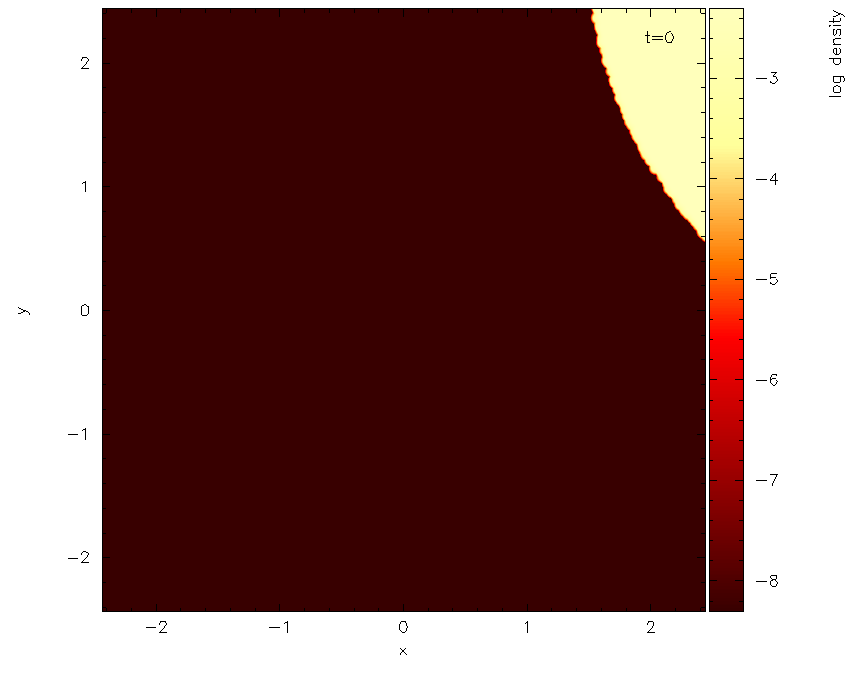
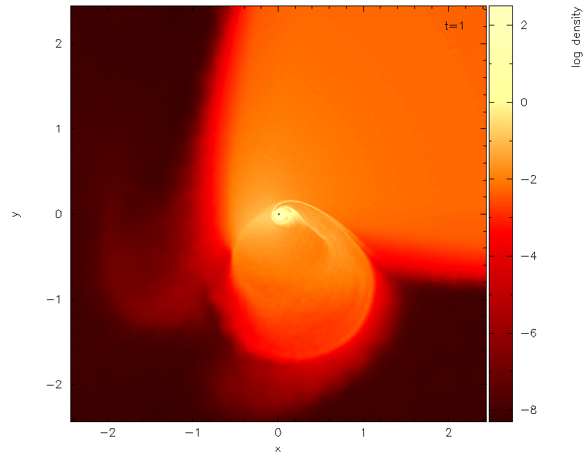
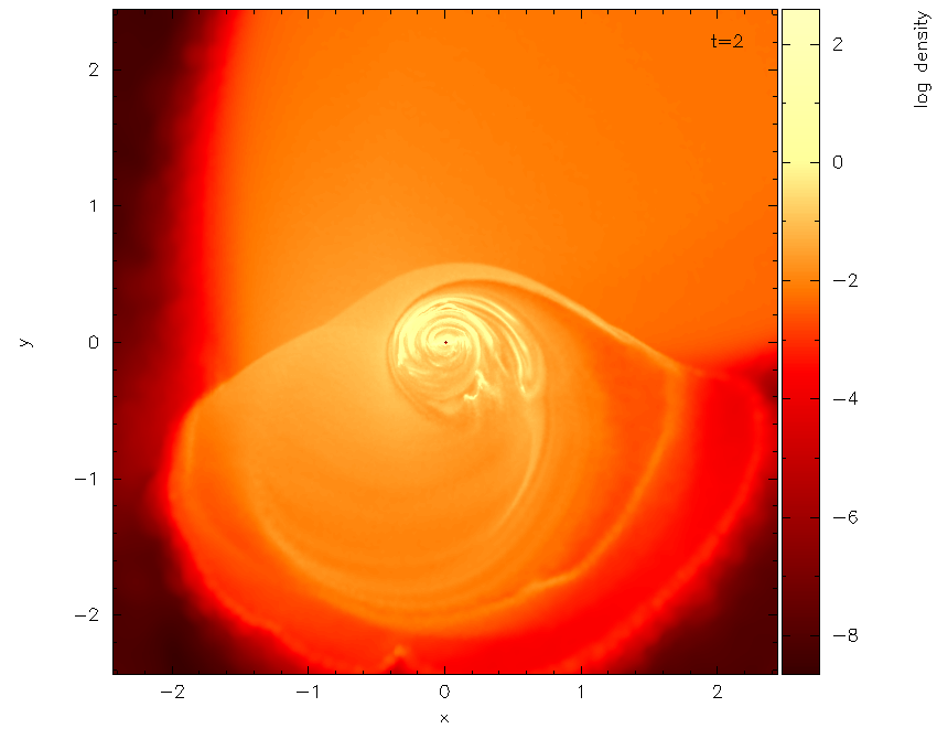
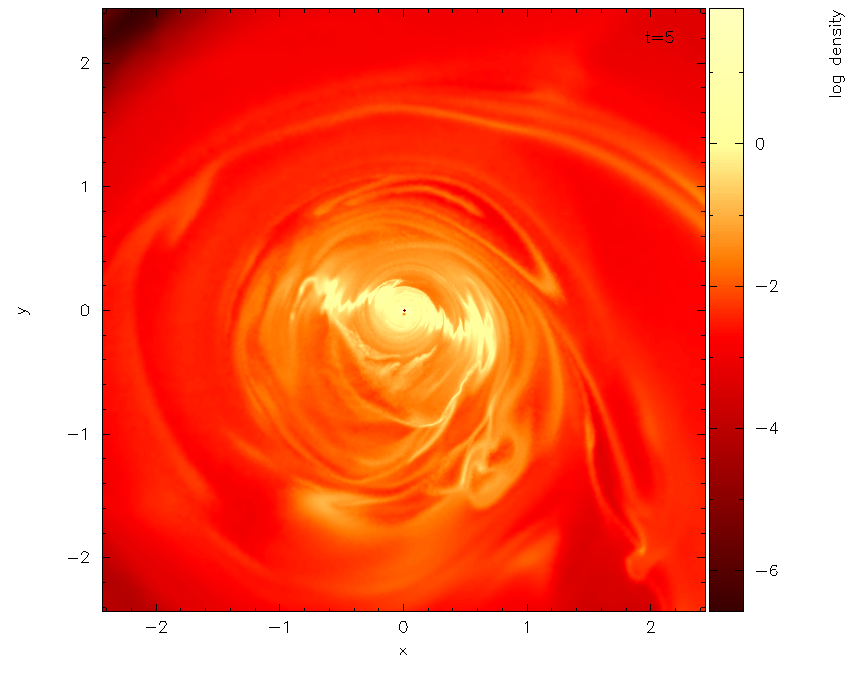
Figure 1.— Snapshots of density structure in the $XY$ plane at different times for V01 model. The times are shown in units of $0.047$ million years, which corresponds to 0.0, 0.047, 0.096 and 0.240 million years for top-left, top-right, bottom-left and bottom-right panels respectively. The unit of length is a parsec, and unit of density is $4.1\cdot 10^{6}\,$cm${}^{-3}\,m_{u}$.

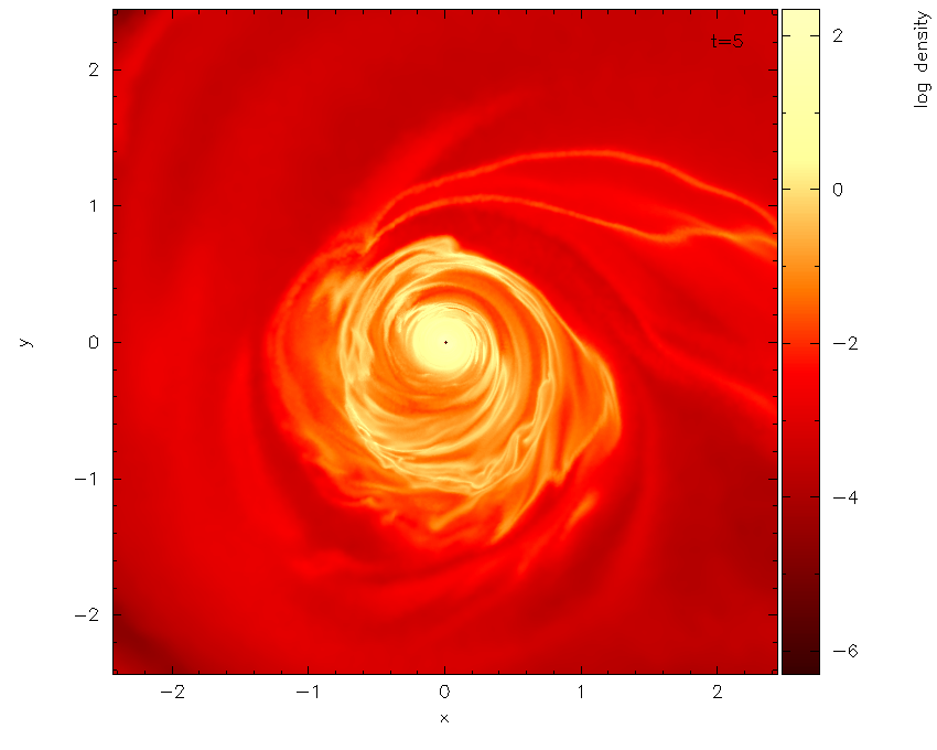
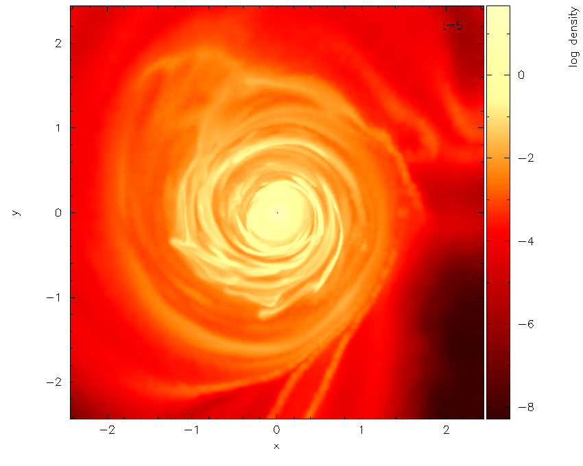
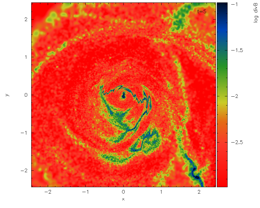
Figure 2.— Density snapshot in the $XY$ plane at the of V02 (top left-panel) and C01 (top right-panel) simulations. As in Fig. 1, the unit of length is a parsec, and density is shown in units of $4.1\cdot 10^{6}\,m_{u}/$cm³. The bottom left and right panels show density profile in $XY$ plane at the end of V01 simulation and the associated divergence error, divB $=|\nabla\cdot{\bf B}|h/|{\bf B}|$ where $h$ is cell size, respectively.

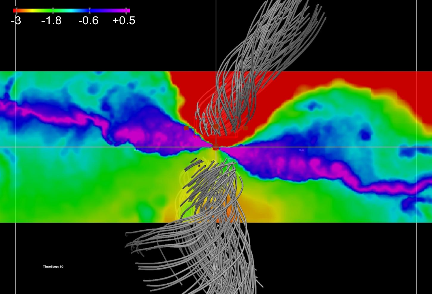
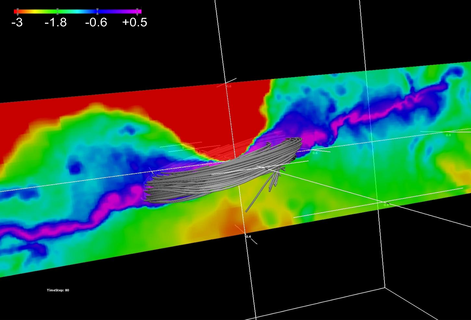
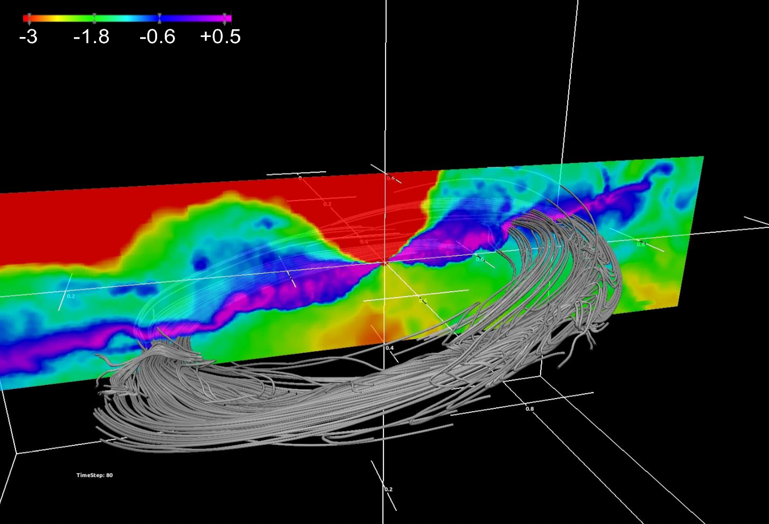
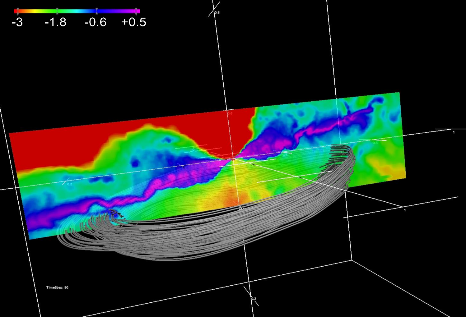
Figure 3.— This figure shows magnetic field geometry in different regions of the disk. The density is shown in the $XZ$ plane, with values given in $\log(\rho/(4.1\cdot 10^{6}{\rm cm}^{3}/m_{u})$. The top two panels show magnetic field geometry in the central region of the disk ($R\sim 0.1\,$pc), whereas two bottom panel focus on outer regions of the disk ($R\sim 0.5\,$pc). While magnetic field geometry is mostly uniform, the gas density show irregular structure.

Table 1This table shows geometry of initial conditions: Column 1 (ID) is the name of a run, Column 2 ($R_{\rm cl})$ show adius of a cloud, Column ($v_{x}$) is cloud infall speed in km/s, and finally last coumn ($b$) is the cloud’s impact parameter.

ID	$R_{\rm cl}$ [${\rm pc}]$	$v_{x}$ [${\rm km/s}$]	$b$ [${\rm pc}$]
C01	3.5	120	2
V01	3.5	30	3
V02	3.5	50	3

We conduct three high resolution simulations with $1.6\times 10^{7}$ particles in which a magnetized gas cloud with mass and radius $3.5\,$pc and $8.8\times 10^{4}\,{\rm{M}}_{\odot}$, respectively, is collided with a $3.5\times 10^{6}\,{\rm{M}}_{\odot}\,$SMBH. The geometry of the initial conditions is taken from Alig et al. (2011) and repeated in Table 1; in particular, we use initial conditions from their simulations C01, V01 and V02, where a molecular cloud has an impact parameter of $2\,$pc, $3\,$pc and $3\,$pc respectively. On top of these initial conditions we also impose a uniform magnetic field that threads both the cloud and vacuum regions. The magnetic field strength is such that the resulting magnetization inside the cloud is $\beta=1$, which corresponds to $|B|\approx 100\,\mu$G and dimensionless mass-to-flux ratio $\zeta\approx 5$, where $\zeta=(M/\Phi)/\sqrt{5/(9\pi^{2}G)}\,$(Mouschovias & Spitzer, 1976; Mac Low & Klessen, 2004). This field strength corresponds to the large-scale field in the Galactic Centre (Yusef-Zadeh & Morris, 1987; Morris & Yusef-Zadeh, 1989; Crocker et al., 2010). The initial magnetic field orientation was such that each of the components of magnetic field have the same magnitude, namely $B_{x}=B_{y}=B_{z}=B/\sqrt{3}$. The vacuum is modelled with fluid $10^{6}$ times less dense than the cloud density ($n=0.01\,{\rm{cm}}^{-3}$), which we also use it as a floor density to avoid local density contrasts larger than $\sim 10^{7}$ that our code cannot deal with due to use of single precision floating point arithmetics.

The computational domain is a periodic box with $32\times 32\times 32\,$pc³ volume, which is large enough not to influence physical processes occurring in sub-parsec regions. The mass and distance units were $[M]=10^{5}\,{\rm{M}}_{\odot}$ and $[R]=1\,$pc respectively, which sets the time unit $[T]\approx 0.047\,{\rm{Myr}}$, magnetic field units $[B]\approx 5.40\,$mG, and the speed unit $[V]\approx 20\,{\rm{km/s}}$. The simulation lasted till $T_{\rm{end}}=5.0$, which corresponds to $0.24\,$Myr or $4.7$ orbital periods at $R=1\,$pc. The inner boundary conditions are applied only within $0.02\,$pc from the SMBH, which we regard as the inner disk boundary, as follows. Any particle within $0.01\,$pc is removed from the computational domain, and in the transition region between $0.01\,$pc and $0.02\,$pc we set the density to the floor value, and both the velocity and the magnetic field to zero.

3. Results

3.1. Geometry of the collision

A collision between a molecular cloud and a supermassive black hole is a violent event occurring on dynamical time-scale. Since fluid elements generally have non-zero angular momentum, the natural outcome of such an event is a formation of a disk. Hydrodynamical simulations of such collision event robustly show a formation of an eccentric disk around SMBH with the disk geometry being dependent on the initial conditions (Alig et al., 2011). Our aim in this work is to study similar event but in strongly magnetised regime in which the initial magnetic pressure in the cloud is in equipartition with the gas thermal pressure.

In Fig. 1 we show snapshots of the gas density in the $XY$ plane at $t$=0, 47, 94, and 240 thousand years. In the first hundred thousand years, the cloud experience a violent collision with the black hole. In particular, the bow-shock, which can be seen in the bottom-left panel as a large curved region with density jump just above the disk, is formed by isothermal shock guards the newly formed inner disk from the destructive effect of the incoming fluid. The outcome of this collision event is a formation of a parsec-size gas disk with irregular density structure. Similar disks where formed in other simulations as can be seen in the top two panels of Fig. 2. This can be contrasted with Alig et al. (2011) where simulations C01 and V01 have final differently shaped gas disks. Finally, in the bottom right panel of Fig. 2 we show the divergence error, $|\nabla\cdot{\bf B}|h/|{\bf B}$ where $h$ is the cell size, in the final snapshot of V01 simulation.

In Fig.3 we show magnetic field geometry in different regions of the disk at the end of the V01 simulation, which corresponds to approximately 150 orbital periods at $R=0.1\,$pc. The top-left panel show magnetic field lines originated in the central region of the disk and extend above and below mid-plane. The magnetic field in this regions is dominated by poloidal components. The top right panel shows mid-plane magnetic field structure in the central region ($R\sim 0.1$pc). The field lines appear regular and tightly winding in azimuthal direction, which is result of strong Keplerian shear inside the disk. In the bottom-left panel, we also show magnetic field in the mid-plane region but further away from the center ($R\sim 0.5\,$pc). While magnetic field is still stretched in azimuthal direction, in contrast to the central regions it shows less regular structure. In the bottom-right panel we show magnetic field in the disk corona, where magnetic field shows regular large-scale azimuthal pattern.

3.2. Vertical structure

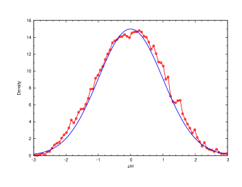
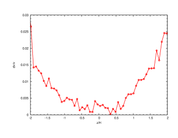
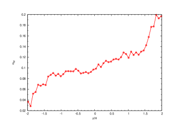
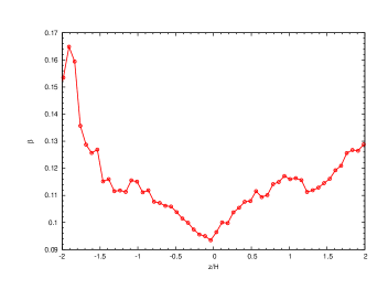
Figure 4.— This figure shows vertical structure of the disk model at the end of the best resolve simulation (V01). The top left panel shows density (red line with open circle) and the fit of the expected density structure (blue line). The top right panel shows the deviation of the azimuthal velocity from the Kerplerian value, the bottom left panel shows Maxwell stress, and the bottom right panel show vertical dependence of the ratio of the gas pressure to the magnetic pressure.

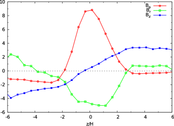
Figure 5.— Vertical dependence of azimuthal (red lines with open circles), radial (blue lines with open squared) and vertical (green line with filled squares) magnetic field components. The dashed and solid lines show low- and high-resolution simulations respectively. Both radial and vertical magnetic field components are $10\times$ magnified.

This section focuses on the vertical disk structure in our simulations. In particular, we studied vertical structure of the disk at $R\approx 0.1\,$pc, which is far enough from the inner boundary and close enough that the disk performed approximately 100 orbital periods by the end of the simulation. One of the crucial properties in magnetised disk simulations is the MRI quality factor, $Q$, which is related to the number of resolution points, e.g. grid-points, particles or mesh-cells, per MRI fastest growing mode wave-length. With this number being too low ($Q\lesssim 8)$, the simulation may fail to faithfully model magneto-rotational instability (e.g. Hawley et al. (2011)). Due to the nature of our simulations, it was impossible a priori to identify which of our simulations can faithfully model long-term disk evolution. As a result, we computed MRI quality factors in vertical and azimuthal directions at the end of our simulations, and check which of the simulations were able to resolve MRI. Namely, we compute $Q_{z}=\lambda_{z}/h$ and $Q_{\phi}=\lambda_{\phi}/h$, where $h$ is the size of a resolution element and $\lambda_{z,\phi}\approx 2\pi|B_{z,\phi}|/(\sqrt{\rho}\Omega)$.

Table 2MRI quality factor for each of our simulations

ID	$Q_{z}$	$Q_{\phi}$
C01	3	26
V01	11	60
V02	6	48

In Table 2 we show vertically averaged quality factors at $R\approx 0.1\,$pc. This table demonstrates that all simulations have $Q_{\phi}\gtrsim 8$, which means they can faithfully model non-axisymmetric MRI. However, only V01 simulation qualifies when it comes to axisymmetric MRI, and therefore we focus our study of vertical structure on this simulation.

We compute scale-height, $H$, at this radius by fitting an isothermal density profiles in approximately two scale-heights. The resulting scale-height is $H\approx 0.01$, which gives $H/R\approx 0.1$ (top-left panel in Fig. 4). The radial temperature dependence is expected to produce disks with the scale height $H/R=0.03\,\sqrt{1+\beta^{-1}}$ which, for $\beta^{-1}=P_{\rm m}/P_{\rm g}\approx 10$ found at $R=0.1\,$pc, gives

We studied vertical structure of the disk in V01 simulation at $R\approx 0.1\,$pc, which is far enough from the inner boundary and close enough that the disk performed approximately 100 orbital periods by the end of the simulation. We compute scale-height, $H$, at this radius by fitting an isothermal density profile in approximately two scale-heights. The resulting scale-height is $H\approx 0.01$, which gives $H/R\approx 0.1$ (top-left panel in Fig. 4). The radial temperature dependence is expected to produce disks with the scale height $H/R=0.03\,\sqrt{1+\beta^{-1}}$ which, for $\beta^{-1}=P_{\rm m}/P_{\rm g}\approx 10$ found at $R=0.1\,$pc, gives $H/R\approx 0.1$, consistent with the simulation data (bottom-right panel in Fig. 4). We also studied the deviation of azimuthal velocity form the Keplerian velocity at $R=0.1\,$pc as a function of height, and found that azimuthal velocity variations are less than a percent for $|z|<H$ (top-right panel in Fig. 4). It is therefore justifiable to assume that the disk angular velocity is constant on cylinders. Finally, in the bottom left panel of the Fig. 4 we show Maxwell stress $\alpha_{M}=-\langle B_{r}B_{\phi}\rangle/P_{\rm tot}$ which is approximately $0.1$ within the scale-height.

In Fig. 5 we show azimuthally averaged magnetic field. This figure show that the magnetic field is confined within few scale-heights of the mid-plane. The magnetic field is dominated by the azimuthal component that is an order of magnitude larger than the radial one. Vertical component, $B_{z}$, is much smaller compared to both $B_{r}$ and $B_{\varphi}$ for $|z|\lesssim\,H/2$ (in this figure both $B_{r}$ and $B_{z}$ strength are magnified by a factor of 10).

All of our simulations show similar vertical confinement of the field, which can be interpreted as a result of the disk formation: a combination of isothermal shocks that amplify magnetic field and Keplerian shear which generates strong azimuthal field component. However, we would like to stress that the field confinement in our best resolved model (V01) is in a good agreement with Johansen & Levin (2008) – hereafter referred to as JL, who find similar results in their shearing box models. In the JL shearing-box simulations, which were performed with a grid-based Pencil Code, the disk field was initially in equipartition with the gas pressure, but evolved by Parker and magnetorotational instabilities to a magnetic field configuration in the vertical direction similar to what we see in our disk which is formed via a collision of a magnetized gas cloud with the black hole. It is significant that the two simulations that are so different in their approach give vertical structure of $B_{\varphi}$ that is in a good agreement with each other. In particular, the azimuthal component changes sign at 2-3 scale-heights above the mid-plane, and the strength of the mid-plane field is ten times the value of the reversed field.

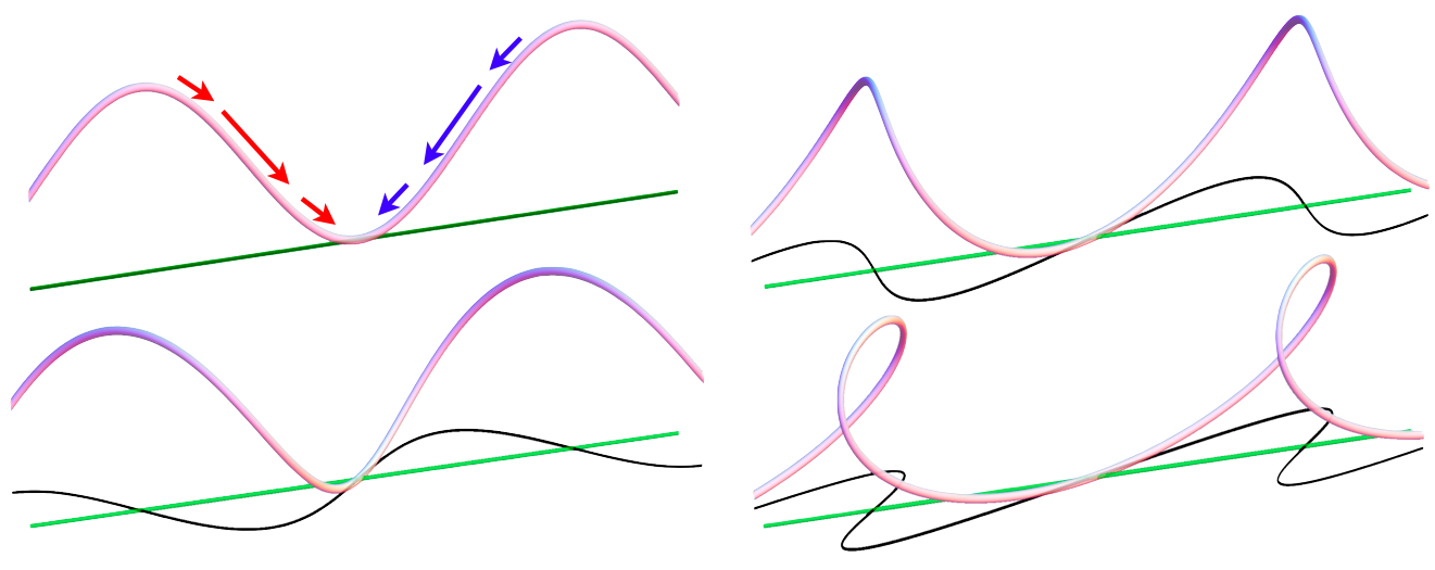
Figure 6.— Sketch of the evolution of a magnetic field line subject to Parker instability, Coriolis force and Keplerian shear. The green straight tube in all panels shows the original field line along $\varphi$ direction in the mid-plane, the white-blue 3D tube depicts the actual field line, and its projection onto the $r-\varphi$ plane is shown in black. The top-left panel shows the undulant distortion of the original field line due to Parker instability in the $\varphi-z$ plane. The fluid elements that slide along the field lines (red and blue arrows) towards the mid-plane are acted upon by the Coriolis force transforming the field line into a helical form. Projection of the field line onto $r-\varphi$ plane shows creation of a radial component (bottom-left). Stretching of the radial component by Keplerian shear regenerates the azimuthal component (top-right). Finally, subsequent stretching of the line generates oppositely oriented magnetic field above mid-plane and increases the strength of the azimuthal component of magnetic field in the mid-plane (bottom-right).

It is likely that the process responsible for flux confinement is of a similar nature as described in JL. We sketch it in Fig. 6. The strong azimuthal magnetic field is subject to Parker instability. As the fluid elements slide along the field line towards the mid-plane (top-left) they are acted upon by the Coriolis force (Hanasz et al., 2002), and due to this the line becomes helical (bottom-left). This generates radial field, which via Keplerian shear regenerates the azimuthal field that was lost to Parker instability (top-right). Further shearing generates oppositely oriented azimuthal field above the mid-plane which reconnects with the field of the original orientation. This decreases its magnitude or even reverses its direction, whereas the field at the mid-plane is amplified while maintaining its original direction (bottom-right).

3.3. Radial structure

The radial evolution of the disk is driven by the flow of matter from the outer to the inner regions. This flow is enabled by the effective viscosity from magnetohydrodynamical stresses. Within the viscous time-scale, the disk reaches steady radial structure which is computed by applying conservation laws and theory of steady thin disks (e.g. Frank et al., 2002). Here we present some numerical evidence for an extra constraint, the conservation of azimuthal magnetic flux, $\Phi=\int\,B_{\varphi}\,dS$ where $dS\,=dz\,v_{\rm{r}}\,dt$. The set of equations that describe disk’s radial structure is

$$\dot{M} = 2\pi\,R\,\Sigma\,v_{\rm{r}},$$ (1)

$$\dot{\Phi} = 2H\,B_{\varphi}\,v_{\rm{r}},$$ (2)

$$\dot{M} = 3\pi\,\alpha_{\rm{acc}}\,\Sigma\,H^{2}\,\Omega.$$ (3)

Here, Eq. (2) describes the frozen-in condition of magnetic field. In what follows we assume that the right hand side of these equations are constants for steady-state disks. We also assume that accretion viscosity $\alpha_{\rm acc}$ is set by Maxwell stresses

$$\alpha_{\rm{acc}}=\alpha_{\rm{m}}=-\frac{\langle B_{r}\,B_{\varphi}\rangle}{4\pi\,P},$$ (4)

where $P=\Omega^{2}\,H\,\Sigma$ is the total pressure. The disk scale-height is

$$H=H_{0}\sqrt{1+\beta^{-1}},$$ (5)

where $H_{0}=c_{\rm{s}}/\Omega$ is a hydrodynamical scale-height. According to the numerical results from the previous section, the magnetic pressure is entirely dominated by $B_{\varphi}$, which gives $P_{\rm{m}}\approx\,B_{\varphi}^{2}/8\pi$.

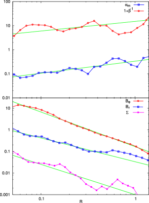
Figure 7.— Radial structure of strongly magnetized disks in our simulations. The upper panel displays disk magnetization, (red line with open circles) and dimensionless viscosity generated by Maxwell stresses (blue line with open squares). The lower panel shows radial dependence of surface density (magenta line with filled squared), and mid-plane $B_{\varphi}$ (red line with open circles) and $B_{r}$ (blue line with open squares); $B_{z}$ has the same scaling and magnitude as $B_{r}$ and is not shown here. The green lines show expected radial dependence from our analytical model.

Using these equations and noting that $(1+\beta)\,B_{\varphi}^{2}/8\pi\,=\Omega^{2}\,H\,\Sigma$, we derive the radial dependence of disk scale-height

$$\frac{H}{R}\,=\,\left(\frac{3\pi^{2}\,G\,\dot{M}\,(1+\beta)}{40\,\alpha_{\rm{m}}\,\zeta^{2}\,(\Omega\,R)^{3}}\right)^{\frac{1}{5}},$$ (6)

where we write $\dot{\Phi}=\sqrt{5/(9\pi^{2}G)}\dot{M}/\zeta$. In the limit, $\beta\ll 1$ the radial dependence of disk magnetization is

$$\beta^{-1}\,=\,\left(\frac{3\pi^{2}\,G\,\dot{M}}{40\,\alpha_{\rm{m}}\,\zeta^{2}(\Omega\,R)^{3}}\right)^{\frac{2}{5}}\left(\frac{R}{H_{0}}\right)^{2}.$$ (7)

In a general case, $H_{0}$ is self-consistently computed by solving radiative transfer equation in the vertical direction. Therefore, the magnetization depends on the thermal properties of the disk. However, in our simulations $H_{0}\,=\,0.03\,R$ from which we have $\beta^{-1}\propto\,R^{3/5}\,\alpha_{\rm{m}}^{-2/5}$.

Since the radial dependence of $\alpha_{\rm{m}}$ is not possible to establish from the first principles, we obtain it empirically. In our numerical experiments $\alpha_{\rm{m}}\propto\,R^{1/2}$ is consistent with the data. This relationship predicts that the disk magnetization should decrease with radius, $\beta^{-1}\propto\,R^{2/5}$, in agreement with our simulations (upper panel in Fig. 7). This radial dependence of $\alpha_{\rm{m}}$ is specific to our simulations which we use for consistency check. However, a similar dependence was found by Flock et al. (2011) in the case of weakly-magnetised disks. In a realistic disk, however, we expect that $\alpha_{\rm{m}}$ is a function of the local $\beta$, which will be subject of subsequent research.

Using equations above, we derive the radial dependence of $B_{\varphi}$, $B_{r}$ and $\Sigma$. To derive $B_{r}$, we use the fact that in our disks the Maxwell stresses in Eq. (4) are dominated by the mean field, $\langle{B_{r}B_{\varphi}}\rangle\approx\langle{B_{r}}\rangle\langle{B_{\varphi}}\rangle$. The resulted radial dependences are

$$\Sigma = \left(\frac{1600}{2187\pi^{9}}\frac{\dot{M}^{3}\zeta^{4}}{G^{2}(1+\beta)^{2}}\right)^{\frac{1}{5}}\frac{(\Omega\,R)^{\frac{1}{5}}}{\alpha_{\rm{m}}^{3/5}R}\propto\,R^{-\frac{7}{5}},$$ (8)

$$B_{\varphi} = \left(\frac{512\sqrt{5}}{27\pi}\frac{\dot{M}^{2}\zeta}{\sqrt{G}(1+\beta)^{3}}\right)^{\frac{1}{5}}\frac{(\Omega\,R)^{\frac{4}{5}}}{\alpha_{\rm{m}}^{2/5}R}\propto\,R^{-\frac{8}{5}},$$ (9)

$$B_{r} = \frac{\alpha_{\rm{m}}}{2}B_{\varphi}\propto\,R^{-\frac{11}{10}}.$$ (10)

These equations are consistent with our simulations throughout most parts of the disk (bottom panel in Fig. 7), except in the regions close to the disk inner boundary. We also do not expect the model to hold for $R\gtrsim 0.4\,$pc, where the viscous time estimated using steady thin disk approximation is much larger than the duration of simulation. Agreement with the analytical model beyond this radius implies that disk evolution there occurs at higher than viscous rate derived from the steady thin disk theory. We also note that the gas density distribution in the disk is not steady, but exhibits clumpy and filamentary structures (right panel in Fig. 3). This is also reflected in the irregularity of the surface density profile in Fig. 7. Nevertheless, agreement of radial dependence between the model and simulations indicates that azimuthal magnetic flux is conserved in MLADs during accretion.

Table 3Accretion rate and effective viscosity

$R\,$[pc]	$\dot{M}\,$[M⊙/yr]	$\alpha_{\rm{acc}}$	$\alpha$
0.05	0.035	0.06	0.03
0.1	0.066	0.09	0.14
0.2	0.070	0.22	0.18
0.4	0.085	0.37	0.31

To verify that the mass accretion is physical, we extract azimuthally and vertically averaged $\Sigma$, $H$, $\dot{M}$ at different radial locations and use Eq. 3 to calculate $\alpha_{\rm{acc}}=\dot{M}/(3\pi\Sigma\,H^{2}\Omega)$. If the accretion is driven by magnetohydrodynamical stresses, this value should be comparable to azimuthally and vertically averaged sum of Maxwell and Reynolds stresses ($\alpha$). We show results in Tab. 3, which shows good agreement between measured ($\alpha$) and derived viscosity ($\alpha_{\rm acc}$) coefficients. This reinforces our confidence that the mass accretion is indeed driven by magnetohydrodynamical stresses. Finally, using data from this table we estimate viscous timescale for a parsec size accretion disk to be $t_{\rm visc}=(R/H)^{2}\alpha^{-1}\Omega^{-1}\approx 10^{6}\,$ years, where we use $\alpha=0.2$ and $H/R=0.2$ at $R=1$ pc.

4. Fragmentation

The striking result that $\Sigma$ and $H$ do not depend on the thermal properties of MLAD allows a robust estimate of its macroscopic gravitational stability. Its fragmentation boundary is determined by two parameters: $\dot{M}$ and dimensionless mass-to-flux ratio $\zeta$. The latter one allows to compute magnetic flux accretion rate from the mass accretion rate, $\dot{\Phi}\propto\dot{M}/\zeta$, since the magnetic field is frozen in the fluid. Using Eq. (6) and Eq. (8), the Toomre-$Q$ parameter is (Toomre, 1964; Goldreich & Lynden-Bell, 1965)

$$Q=\frac{\Omega^{2}\,H}{\pi\,G\,\Sigma}=\left[\frac{6561\pi^{6}}{64000}\frac{(1+\beta)^{3}}{G^{2}\,\dot{M}^{2}\,\zeta^{6}}\alpha_{\rm{m}}^{2}(\Omega\,R)^{6}\right]^{\frac{1}{5}}.$$ (11)

If we write $\dot{M}$ in terms of Eddington luminosity, $l_{\rm{E}}=L/L_{\rm{Edd}}$, and radiative efficiency, $\epsilon=L/(\dot{M}c^{2})$,

$$\dot{M}=\frac{4\pi GM}{\kappa_{\rm{es}}c}\frac{l_{\rm{E}}}{\epsilon},$$ (12)

where $\kappa_{\rm{es}}\approx 0.4\,{\rm{c}m}^{2}/{\rm{g}}$ is electron scattering opacity, and $c$ is speed of light, we obtain

$$Q=\left[\frac{6561\pi^{4}}{4^{5}10^{3}}\frac{\kappa^{2}\,c^{2}(1+\beta)^{3}}{G^{2}}\frac{\alpha_{\rm{m}}^{2}}{\zeta^{6}}\left(\frac{\epsilon}{l_{\rm{E}}}\right)^{2}\Omega^{2}\right]^{\frac{1}{5}}.$$ (13)

Using Eq. (13) we find the fragmentation boundary beyond which $Q<1$,

$$R_{\rm{frag}}\approx 2.09\left(\frac{M_{6}\,\alpha_{0.1}^{2}\,\epsilon_{0.1}^{2}}{\zeta_{10}^{6}\,l_{\rm{E}}^{2}}\right)^{\frac{1}{3}}\,{\rm{pc}},$$ (14)

where we used $\epsilon=0.1\,\epsilon_{0.1}$, $\alpha_{\rm{m}}=0.1\,\alpha_{0.1}$, $\zeta=10\,\zeta_{10}$ and $M=10^{6}\,M_{6}\,{\rm M}_{\odot}$. The radial dependence of enclosed mass and $H/R$ within the fragmentation radius is given by

$$\frac{M_{\rm{disk}}}{M} = \frac{\sqrt{10}\pi\,r^{9/10}}{3\zeta}\approx 0.331\,\frac{r^{9/10}}{\zeta_{10}},$$ (15)

$$\frac{H}{R} = \frac{3\pi\,r^{3/10}}{2\sqrt{10}\zeta}\approx 0.149\,\frac{r^{3/10}}{\zeta_{10}},$$ (16)

where we define $r=R/R_{\rm{frag}}$. It is worth noticing, that at the fragmentation boundary, $M_{\rm{disk}}$ and $H/R$ depend only on mass-to-flux ratio.

In future work we will use our MLAD solution to model observations of AGN accretion disk. Here, we briefly consider a parsec-sized disk in NGC1068 (Jaffe et al., 2004) as an eaxmple. This Seyfert 2 galaxy hosts an $\sim 10^{7}\,{\rm{M}}_{\odot}$ SMBH with a disk extending to a distances of $\sim 1\,$pc. The observed upper bound for $H/R\sim 0.6$ and the hydrogen column density $N_{\rm{H}}\sim 10^{25}\,{\rm{cm}}^{-2}\,$(Matt et al., 2004; Köhler & Li, 2010), and its luminosity is $\sim 0.4\,L_{\rm{Edd}}$ (Pier et al., 1994) . Here, we assume that this SMBH accretes at Eddington rate ($l_{\rm{E}}\approx 1$) with 10% radiative efficiency ($\epsilon_{0.1}\approx 1$); we set $\alpha_{0.1}=1$. We find that by setting $\zeta=3$, we are able to obtain values for disk thickness and column density that are consistent with observations. For this parameters, the MLAD thickness at the edge of such disk is $H/R\approx 0.15$. While this is lower than the observed value, it is plausible that strong magnetic fields contribute toward increasing disk thickness. Finally, using the enclosed disk mass at this location and assuming that the disk consists purely of atomic hydrogen, we estimate $N_{\rm{H}}\approx 1.3\times 10^{25}\,{\rm{cm}}^{-2}$ which is consistent with the observational data. Furthermore, the fragmentation boundary is located at $\approx 50\,$pc, which indicates that a parsec-sized disk is stable to clumping. This MLAD model predicts that such disk should have magnetic field strength of $\sim 100\,$mG.

5. Conclusions

In this paper we produce from first principles dynamically stable models of accretion disks in a state of magnetic levitation. We show that such disks are the natural outcome of in-fall of a massive magnetized molecular cloud onto supermassive black hole. Such magnetically-levitating accretion disks (MLADs) enable large accretion rates due to the large scale-height and $\alpha\gtrsim 0.1$. In our simulations, the geometry and strength of the large-scale magnetic field are stable for at least $0.24\,$Myr, corresponding to several hundred orbits at the disk inner edge. With measured accretion rates of $\approx 0.05\,{\rm M}_{\odot}$/yr, this is more than 10% of the disk lifetime, supporting the claim that such magnetic fields structure is possibly long lived. The viscous time-scale of such magnetically levitating disk is estimated to be few million years. Interestingly, this feature may help solve a theoretical problem that was recently identified by Alexander et al. (2011) with respect to the formation of the stellar disc in our Galactic Centre. These authors show that if, as according to the currently accepted scenario (Levin & Beloborodov, 2003; Nayakshin et al., 2007; Bonnell & Rice, 2008), the stellar disc formed as a result of fragmentation of the massive gaseous accretion disc several million years ago, then a substantial gaseous remnant of the accretion disc should survive to the present epoch, due to the expected long viscous time of the standard Shakura-Syunyaev thin discs. Such a remnant is not observed. On the other hand, the expected short lifetime of the MLAD, may solve the problem of the missing remnant gas disk.

A unique property of magnetically-levitating disks is that their surface density and scale-height are independent of the disk’s thermal structure. This is expected because thermal effects are superseded by magnetic properties in determining disk structure. Magnetic levitation allows the disk to withstand its own self-gravity to large distances. A strong dependence of the fragmentation radius on the mass-to-flux ratio of the parent cloud permits a scenario in which a tidal disruption of a magnetized cloud forms a magnetized gas ring. The inner parts spreads inwards on a time-scale determined by global magnetic stresses which fuel fast accretion onto the central supermassive black hole, while the outer part fragments into stars.

A proper understanding of the field confinement requires both local and global analysis. In accordance with JL, the field confinement appears to be a local phenomenon and its stability is likely to depend on the relative strength of vertical and azimuthal magnetic field, which itself depends on both kinematics and magnetisation of the infalling matter. However our simulations show that there are non-local processes which generate a global coherent magnetic field structure. Its topology and strength is very important for accretion flows near black-hole horizons (Beckwith et al., 2008; Tchekhovskoy et al., 2011; Tchekhovskoy & McKinney, 2012). Therefore it is also important to understand the long-term evolution of the field topology across several decades in the disc radius we believe that both local and global simulations are essential to our understanding of MLADs.

Appendix A Numerical method

In this appendix we demonstrate the ability of our numerical scheme to model MHD flows. Our numerical method combines a moving-mesh approach (Trease, 1988; Springel, 2010) with a weighted particle MHD scheme (Gaburov & Nitadori, 2011). At every time-step a Voronoi mesh is re-built on the set of particles which is used to solve equations of ideal MHD in the same way as in the weighted particle scheme. Similar approach has also been attempted in TESS (Duffell & MacFadyen, 2011) and AREPO (Pakmor et al., 2011) moving-mesh codes. In contrast to these two approaches but similarly to Gaburov & Nitadori (2011), we add a source term to the induction equation that restores Galliean invariance of scheme in the case of $\nabla\cdot{\rm B}\neq 0$. This proved to be crucial to stabilize the numerical scheme in the presence of strongly magnetised super-alfvenic flows. The numerical code is pubcly available. Here, we present validation of our numerical method by means of two test problems: propagation of circularly polarized Alfven wave and the linear regime of magneto-rotational instability in a cylindrical disk.

A.1. Circularly polarized Alfven wave

This problem was first presented by Tóth (2000) as an exact non-linear test problem for ideal MHD. Following Tóth (2000) we set the following initial conditions. We use a periodic three-dimensional computational domain with the total number of particles equal to $N_{\rm tot}=N_{x}\times N_{x}/2\times 16$, where $Nx=16,32,64$ and $128$. Particles were initially randomly sampled from a uniform distribution and regularized with the Lloyd’s algorithm (e.g. Springel (2010)). The initial conditions are $\rho=1$, $P_{\rm gas}=0.1$, $B_{x}=1$, $v_{x}=1$, $B_{y}=v_{y}=0.1\sin(4\pi x)$, $B_{z}=v_{z}=0.1\cos(4\pi x)$, which fits two wave-length into the $x$-direction. With these initial conditions, the wave-length is resolved with an average of $6,13,26$ and $52$ mesh-points from the lowest to the highest resolution respectively. The apparent discrepancy from the expected resolutions of $8,16,32$ and $64$ mesh-cells per wave-length is due to the initial particle distribution is not being a simple cubic lattice, but rather a random distribution which was relaxed by the Lloyd’s algorithm. This relaxed distribution consists of mesh-cells which can be approximated by regular convex polyhedra with large number of faces ($\gtrsim 15$). The effective size of such mesh-cell can be approximated by the diameter of a sphere having the same volume as the cell itself, and this in turn increases the effective size of the mesh-cell by approximately $\sqrt[3]{6/\pi}\approx 1.24$ compared to a simple cubic cell, while keeping the total volume the same.

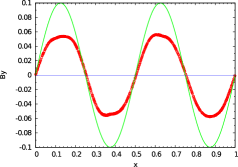
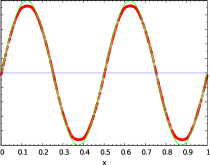
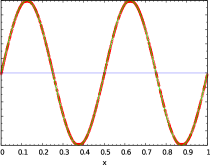
Figure 8.— The circularly polarized Alfven wave after five crossings of computational domain. The panels show the $y$-component of the magnetic field as a function of $x$-coordinate. The solid line demonstrates exact solution, while the open circles show the result of simulations. In the left-most, middle and right-most panels, the wavelength is resolveid with an average of $13$, $26$ and $52$ meshpoints respectively.

In Fig. 8 we compare the simulated results to the analytical solution. It can be seen that lower resolution simulations have more dissipation but do not introduce phase error in the solution. The dissipation is not the result of the underlying Riemann-solver or a reconstruction method, but rather that of non-linear monotonicity constraints on the linear reconstruction model which is required for a stable description of discontinuities. The side effect of these is the constraint is that it forces the scheme to be first order accurate at extrema (van Leer, 1979; Iwasaki & Inutsuka, 2011).

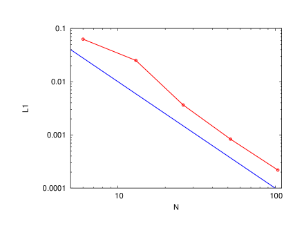
Figure 9.— The $L_{1}$ error as a function of resolution for circularly polarized Alfven wave. The open circles connected by the red solid line show results of simulations, and the blue solid line is expected dependence for the second order scheme $\propto O(N^{-2})$. The vertical axis show $L_{1}$ error in the solution as a faction of number of meshpoints, $N$, per wavelength.

In Fig. 9 we show $L_{1}$ error of the simulations solution as a function of the number of meshpoints per unit wavelength. Here, the $L_{1}$ error is defined as $L_{1}=1/N\sum_{i}|f_{i}-f_{\rm ex}|$ where sum is carried out over all $N$ mesh-cells, and $|f_{i}-f_{\rm ex}|$ is absolute deviation of the value in a cells, $f_{i}$, from the corresponding exact solution, $f_{\rm ex}$. The result demonstrates that the convergence for this problem is consistent with the second-order scheme.

A.2. Magneto-rotational instability in non-stratified cylindrical disk

In this problem we study the ability of our code to reproduce analytical growth-rates of axisymmetric magneto-rotational instability. Our computational domain consist of the three-dimensional non-stratified cylindrical disk. The inner and outer radii of the disk are equal to $R=1$ and $R=8$, and the thickness of the disk is $H=1$. We use periodic boundary conditions in $z$ direction, and outflow boundaries at $R=1$ and $R=8$. The total computational domain is a box with size $[16.6\times 16.6\times 1]$.

We simulated three models with an average $14,20$ and $28$ meshpoints in $z$-direction. The initial density is set to unity, and we used isothermal equations of state with constant sound speed $c_{s}=0.1$. The gravitational potential is equal to $\phi=-1/R$, where $R=\sqrt{x^{2}+y^{2}}$, and the initial velocity is equal to the Keplerian velocity. Initially, we set a uniform magnetic field in $2<R<4$ annulus of the disk with such strength that results in fastest growth for $n=2$ mode at $R\approx 2$. Namely we have, $B_{x}=B_{y}=0$ and $B_{z}\approx 0.055/n$, where $n=2$. In other words, at $R\approx 2$ the fastest growing MRI mode has the wavelength $\lambda_{\rm MRI}\approx H/2$. In this setup, the $\lambda_{\rm MRI}$ is resolved with approximated $7$, $10$ and $14$ meshpoints in low, medium and high-resolution simulations respectively.

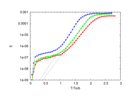
Figure 10.— This figure shows radial magnetic energy in an annulus $2<R<2+1/42$ (vertical axis) as a function of the number of local orbits at $R=2$ (horizontal axis). The solid red line shows time evolution of radial magnetic energy for low resolution simulation (on average 7 meshpoints per $\lambda_{\rm MRI}$), the green dashed and blue dotted lines shows the results for medium (10 meshpoints per $\lambda_{\rm MRI}$) and high resolution (14 meshpoints per $\lambda_{\rm MRI}$). The left and right dotted lines show exponential growth with slopes $0.75\gamma$ and $0.65\gamma$ respectively, where $\gamma=4\pi$.

In Fig. 10 we show time evolution of radial magnetic energy $E=B_{r}^{2}/2$ as a function of the number of orbits at $R=2$ for three different resolutions. All simulations show exponential growth rater after approximately one orbital period, and the low resolution simulations shows growth rate $\approx 0.6\Omega$, whereas the medium and high resolution simulations show growth rate $\approx 0.65\Omega$ and $\approx 0.75\Omega$ respectively.

References

- Alexander et al. (2011) Alexander R. D., Smedley S. L., Nayakshin S., King A. R., 2011, MNRAS, p. 1736
- Alig et al. (2011) Alig C., Burkert A., Johansson P. H., Schartmann M., 2011, MNRAS, 412, 469
- Balbus & Hawley (1991) Balbus S. A., Hawley J. F., 1991, ApJ, 376, 214
- Beckwith et al. (2008) Beckwith K., Hawley J. F., Krolik J. H., 2008, ApJ, 678, 1180
- Begelman & Pringle (2007) Begelman M. C., Pringle J. E., 2007, MNRAS, 375, 1070
- Bonnell & Rice (2008) Bonnell I. A., Rice W. K. M., 2008, Science, 321, 1060
- Brandenburg et al. (1995) Brandenburg A., Nordlund A., Stein R. F., Torkelsson U., 1995, ApJ, 446, 741
- Clyne et al. (2007) Clyne J., Mininni P., Norton A., Rast M., 2007, New J. Phys, 9
- Crocker et al. (2010) Crocker R. M., Jones D. I., Melia F., Ott J., Protheroe R. J., 2010, Nature, 463, 65
- Davis et al. (2010) Davis S. W., Stone J. M., Pessah M. E., 2010, ApJ, 713, 52
- Duffell & MacFadyen (2011) Duffell P. C., MacFadyen A. I., 2011, ApJS, 197, 15
- Flock et al. (2011) Flock M., Dzyurkevich N., Klahr H., Turner N., 2011, ApJ, 735, 122
- Frank et al. (2002) Frank J., King A., Raine D. J., 2002, Accretion Power in Astrophysics: Third Edition
- Gaburov & Nitadori (2011) Gaburov E., Nitadori K., 2011, MNRAS, 414, 129
- Goldreich & Lynden-Bell (1965) Goldreich P., Lynden-Bell D., 1965, MNRAS, 130, 97
- Goodman (2003) Goodman J., 2003, MNRAS, 339, 937
- Hanasz et al. (2002) Hanasz M., Otmianowska-Mazur K., Lesch H., 2002, A&A, 386, 347
- Hawley et al. (2011) Hawley J. F., Guan X., Krolik J. H., 2011, ApJ, 738, 84
- Hirose et al. (2006) Hirose S., Krolik J. H., Stone J. M., 2006, ApJ, 640, 901
- Hobbs & Nayakshin (2009) Hobbs A., Nayakshin S., 2009, MNRAS, 394, 191
- Iwasaki & Inutsuka (2011) Iwasaki K., Inutsuka S.-I., 2011, MNRAS, 418, 1668
- Jaffe et al. (2004) Jaffe W., Meisenheimer K., Röttgering H. J. A., 2004, Nature, 429, 47
- Johansen & Levin (2008) Johansen A., Levin Y., 2008, A&A, 490, 501
- King & Pringle (2007) King A. R., Pringle J. E., 2007, MNRAS, 377, L25
- Köhler & Li (2010) Köhler M., Li A., 2010, MNRAS, 406, L6
- Kolykhalov & Syunyaev (1980) Kolykhalov P. I., Syunyaev R. A., 1980, Soviet Astronomy Letters, 6, 357
- Levin & Beloborodov (2003) Levin Y., Beloborodov A. M., 2003, ApJ, 590, L33
- Lynden-Bell (1969) Lynden-Bell D., 1969, Nature, 223, 690
- Mac Low & Klessen (2004) Mac Low M.-M., Klessen R. S., 2004, Reviews of Modern Physics, 76, 125
- Machida et al. (2000) Machida M., Hayashi M. R., Matsumoto R., 2000, ApJ, 532, L67
- Machida et al. (2006) Machida M., Nakamura K. E., Matsumoto R., 2006, PASJ, 58, 193
- Matt et al. (2004) Matt G., Bianchi S., Guainazzi M., Molendi S., 2004, A&A, 414, 155
- Miyoshi et al. (1995) Miyoshi M., Moran J., Herrnstein J., 1995, Nature, 373, 127
- Morris & Yusef-Zadeh (1989) Morris M., Yusef-Zadeh F., 1989, ApJ, 343, 703
- Mouschovias & Spitzer (1976) Mouschovias T. C., Spitzer Jr. L., 1976, ApJ, 210, 326
- Nayakshin et al. (2007) Nayakshin S., Cuadra J., Springel V., 2007, MNRAS, 379, 21
- Oda et al. (2009) Oda H., Machida M., Nakamura K. E., Matsumoto R., 2009, ApJ, 697, 16
- Pakmor et al. (2011) Pakmor R., Bauer A., Springel V., 2011, MNRAS, p. 1536
- Pariev et al. (2003) Pariev V. I., Blackman E. G., Boldyrev S. A., 2003, A&A, 407, 403
- Paumard et al. (2006) Paumard T., Genzel R., Martins F., Nayakshin S., Beloborodov A. M., Levin Y., Trippe S., Eisenhauer F., Ott T., Gillessen S., Abuter R., Cuadra J., Alexander T., Sternberg A., 2006, ApJ, 643, 1011
- Pier et al. (1994) Pier E. A., Antonucci R., Hurt T., Kriss G., Krolik J., 1994, ApJ, 428, 124
- Price (2007) Price D. J., 2007, Publications of the Astronomical Society of Australia, 24, 159
- Rafikov (2009) Rafikov R. R., 2009, ApJ, 704, 281
- Sanders (1998) Sanders R. H., 1998, MNRAS, 294, 35
- Shakura & Sunyaev (1973) Shakura N. I., Sunyaev R. A., 1973, A&A, 24, 337
- Shibata et al. (1990) Shibata K., Tajima T., Matsumoto R., 1990, ApJ, 350, 295
- Shlosman & Begelman (1987) Shlosman I., Begelman M. C., 1987, Nature, 329, 810
- Shlosman et al. (1990) Shlosman I., Begelman M. C., Frank J., 1990, Nature, 345, 679
- Springel (2010) Springel V., 2010, MNRAS, 401, 791
- Stone et al. (1996) Stone J. M., Hawley J. F., Gammie C. F., Balbus S. A., 1996, ApJ, 463, 656
- Tchekhovskoy & McKinney (2012) Tchekhovskoy A., McKinney J. C., 2012, MNRAS, 423, L55
- Tchekhovskoy et al. (2011) Tchekhovskoy A., Narayan R., McKinney J. C., 2011, MNRAS, 418, L79
- Toomre (1964) Toomre A., 1964, ApJ, 139, 1217
- Tóth (2000) Tóth G., 2000, Journal of Computational Physics, 161, 605
- Trease (1988) Trease H. E., 1988, Computer Physics Communications, 48, 39
- van Leer (1979) van Leer B., 1979, Journal of Computational Physics, 32, 101
- Wardle & Yusef-Zadeh (2008) Wardle M., Yusef-Zadeh F., 2008, ApJ, 683, L37
- Wardle & Yusef-Zadeh (2012) Wardle M., Yusef-Zadeh F., 2012, ApJ, 750, L38
- Yusef-Zadeh & Morris (1987) Yusef-Zadeh F., Morris M., 1987, AJ, 94, 1178