Searches for neutrinoless double beta decay

Abstract

Neutrinoless double beta decay is a lepton number violating process whose observation would also establish that neutrinos are their own anti-particles. There are many experimental efforts with a variety of techniques. Some (EXO, Kamland-Zen, GERDA phase I and CANDLES) started take data in 2011 and EXO has reported the first measurement of the half life for the double beta decay with two neutrinos of ¹³⁶Xe. The sensitivities of the different proposals are reviewed.

1 Introduction

For many isotopes like ⁷⁶Ge $\beta$ decay is energetically forbidden, but double beta decay ($2\nu\beta\beta$) is allowed

$$(A,Z)\rightarrow(A,Z+2)+2e^{-}+2\bar{\nu_{e}}$$ (1)

This was suggested very early [1] and - following the idea of Majorana that neutrinos could be their own anti-particle [2] - also the possibility of neutrinoless double beta decay $0\nu\beta\beta$ was anticipated shortly afterwards [3] (for a review see [4, 5]). The latter case is very interesting since lepton number is violated and it would establish that the neutrino is its own anti-particle. The experimental signature in this case is a line at the $Q_{\beta\beta}$ value of the decay if the sum of the electron energies is plotted.

Searches for double beta decay date back to the beginning of nuclear physics and nowadays more than a dozen large scale experimental programs are suggested. These programs are compared in this article and also the status of theoretical matrix element calculations is discussed. For general reviews the reader is refered to the literature, e.g. [6, 7, 8].

There are also other related processes like double positron decay or double electron capture processes. While $0\nu\beta\beta$ is already a suppressed process, the other decays are expected to be even rarer unless there is some resonance enhancement [9, 10, 11, 12]. In this article only $0\nu\beta\beta$ decay searches are discussed.

2 Motivation

The observation of neutrino oscillation establishes that these particles have mass [13]. Since neutrinos have no electric charge, there is no known symmetry which forbids additional terms in the effective Lagrangian beside the standard Dirac mass term $m_{D}$ [7]:

$$-L_{\rm Yuk} = m_{D}\overline{\nu_{L}}\nu_{R}+\frac{1}{2}m_{L}\overline{\nu_{L}}(\nu_{L})^{c}+\frac{1}{2}m_{R}\overline{(\nu_{R})^{c}}\nu_{R}+h.c.$$ (2)

$$= \frac{1}{2}(\overline{\nu_{L}},\,\,\overline{(\nu_{R})^{c}})\left(\begin{array}[]{cc}m_{L}&m_{D}\\ m_{D}&m_{R}\end{array}\right)\left(\begin{array}[]{c}(\nu_{L})^{c}\\ \nu_{R}\end{array}\right)+h.c.$$ (7)

The subscript $L$ stands for the left-handed chiral field $\nu_{L}=\frac{1}{2}(1-\gamma_{5})\,\,\nu$ and $R$ for the right-handed projection $\frac{1}{2}(1+\gamma_{5})\,\,\nu$. The superscript $C$ denotes charge conjugation. The $m_{R}$ term describes therefore an incoming neutrino and an outgoing anti-neutrino, i.e. lepton number is violated by 2 units. The eigen states of the mass matrix are of the form $(\nu+\nu^{c})$. Consequently neutrinos are expected to be - in general - their own anti-particles, i.e. Majorana particles.

What is the best experimental approach to establish that our known neutrinos are Majorana particles? Neutrinos (or anti-neutrinos) are produced in charged weak current reactions and - depending on the charge of the associated lepton - only one chiral projection couples. For example in $\beta$ decay $n\rightarrow p\,e^{-}\,\bar{\nu}_{e,R}$, a right-handed anti-neutrino couples:

$$\bar{\nu}_{e,R}=\bar{\nu}_{e}\frac{1}{2}(1+\gamma_{5})=\sum\limits_{i=1}^{3}U_{ei}(\bar{\nu}_{i,h=+1}+\frac{m_{i}}{E}\bar{\nu}_{i,h=-1})$$ (8)

Here, $U$ is the PMNS mixing matrix, $\nu_{i}$ are the mass eigen states with mass eigen values $m_{i}$, $E$ is the neutrino energy and $h$ stands for the helicity of the anti-neutrino.

For a Dirac particle these anti-neutrinos can only undergo detection reactions like $p\,\bar{\nu}_{e,R}\rightarrow n\,e^{+}$. If, on the other hand, neutrinos are Majorana particles, then the $\nu_{i,h=-1}$ component can undergo the reaction $\nu_{e,L}\,n\rightarrow p\,e^{-}$ with

$${\nu_{e,L}}=\frac{1}{2}(1-\gamma_{5}){\nu_{e}}=\sum\limits_{i=1}^{3}U_{ei}({\nu_{i,h=-1}}+\frac{m_{i}}{E}{\nu_{i,h=+1}})$$ (9)

The rate of this reaction is however suppressed by the factor $(m_{i}/E)^{2}$ which is e.g. $10^{-14}$ for a neutrino mass of 0.1 eV and a neutrino energy of 1 MeV. Thus solar neutrino experiments for example will not be able to establish the nature of neutrinos.

The alternative is the search for $0\nu\beta\beta$ where the neutrino only enters as a propagator $\simeq m_{\beta\beta}/q^{2}=\sum_{i}U_{ei}^{2}\cdot m_{i}/q^{2}$. The coupling strength $m_{\beta\beta}$ is called the effective Majorana mass. Since one mole contains a large number of nuclei, the factor $(m_{i}/E)^{2}$ is compensated. For 35 isotopes double beta decay is the only possible decay mode. The Standard Model allowed decay with two emitted neutrinos ($2\nu\beta\beta$) has been observed for 11 isotopes with half lives between $7\cdot 10^{18}$ y and $2\cdot 10^{21}$ y [14, 15].

Part of the Heidelberg-Moscow experiment claims to have observed $0\nu\beta\beta$ of ⁷⁶Ge with $m_{\beta\beta}\approx 0.2-0.6$ eV [16]. Clearly this needs independent confirmation which poses another motivation for the experimental efforts.

3 Experimental sensitivity

An experiment will observe some background events $\lambda_{\rm bkg}$ which - if this number scales by the detector mass $M$ - is given by

$$\lambda_{\rm bkg}=M\cdot t\cdot B\cdot\Delta E$$ (10)

and possibly signal events

$$\lambda_{\rm sig}=\ln 2\cdot N_{A}\cdot\epsilon\cdot\eta\cdot M\cdot t/(A\cdot T_{1/2}^{0\nu}).$$ (11)

Here $t$ is the measurement time, $B$ the so called background index given typical in cnts/(keV$\cdot$kg$\cdot$y), $\Delta E$ is the width of the search window which depends on the experimental energy resolution, $N_{A}$ is the Avogadro constant, $\epsilon$ the signal detection efficiency, $\eta$ the mass fraction of the $0\nu\beta\beta$ isotope, $A$ the molar mass of this isotope and $T_{1/2}^{0\nu}$ its half life.

Table 1: List of most interesting $0\nu\beta\beta$ isotopes. Half lives are taken from [14, 15] while all other numbers are from [7].

isotope	$G^{0\nu}$	$Q_{\beta\beta}$	nat. abund.	$T_{1/2}^{2\nu}$	experiments
	$[\frac{10^{-14}}{y}$]	[keV]	[%]	[1020 y]
48Ca	6.3	4273.7	0.187	0.44	CANDLES
76Ge	0.63	2039.1	7.8	15	GERDA, Majorana Demonstrator
82Se	2.7	2995.5	9.2	0.92	SuperNEMO, Lucifer
100Mo	4.4	3035.0	9.6	0.07	MOON, AMoRe
116Cd	4.6	2809	7.6	0.29	Cobra
130Te	4.1	2530.3	34.5	9.1	CUORE
136Xe	4.3	2461.9	8.9	21	EXO, Kamland-Zen, NEXT, XMASS
150Nd	19.2	3367.3	5.6	0.08	SNO+, DCBA/MTD

If $\lambda_{\rm bkg}<1$ the experimental sensitivity scales with $M\cdot t$ while for $\lambda_{\rm bkg}>>1$ the e.g. 90%  C.L. limit on the half life (assuming there is no signal) is given by

$$T_{1/2}^{0\nu}(90\%CL)>\frac{\ln 2}{1.64}\frac{N_{A}}{A}\,\epsilon\cdot\eta\cdot\sqrt{\frac{M\cdot t}{B\cdot\Delta E}}.$$ (12)

If systematic errors become important e.g. if the energy resolution is not well known or the assumption of the background shape is not correct, then the sensitivity is reduced.

4 Theoretical considerations

The half life for $0\nu\beta\beta$ is given by [7]

$$[T_{1/2}^{0\nu}]^{-1}=G_{0\nu}(Q_{\beta\beta},Z)|M_{0\nu}|^{2}\frac{m_{\beta\beta}^{2}}{m_{e}^{2}}$$ (13)

Here $G_{0\nu}$ is the calculable phase space factor (Tab. 1), $m_{e}$ is the electron mass and $M_{0\nu}$ is the nuclear matrix element whose calculation is difficult and can only be done using approximations. For a review see for example [6, 8].

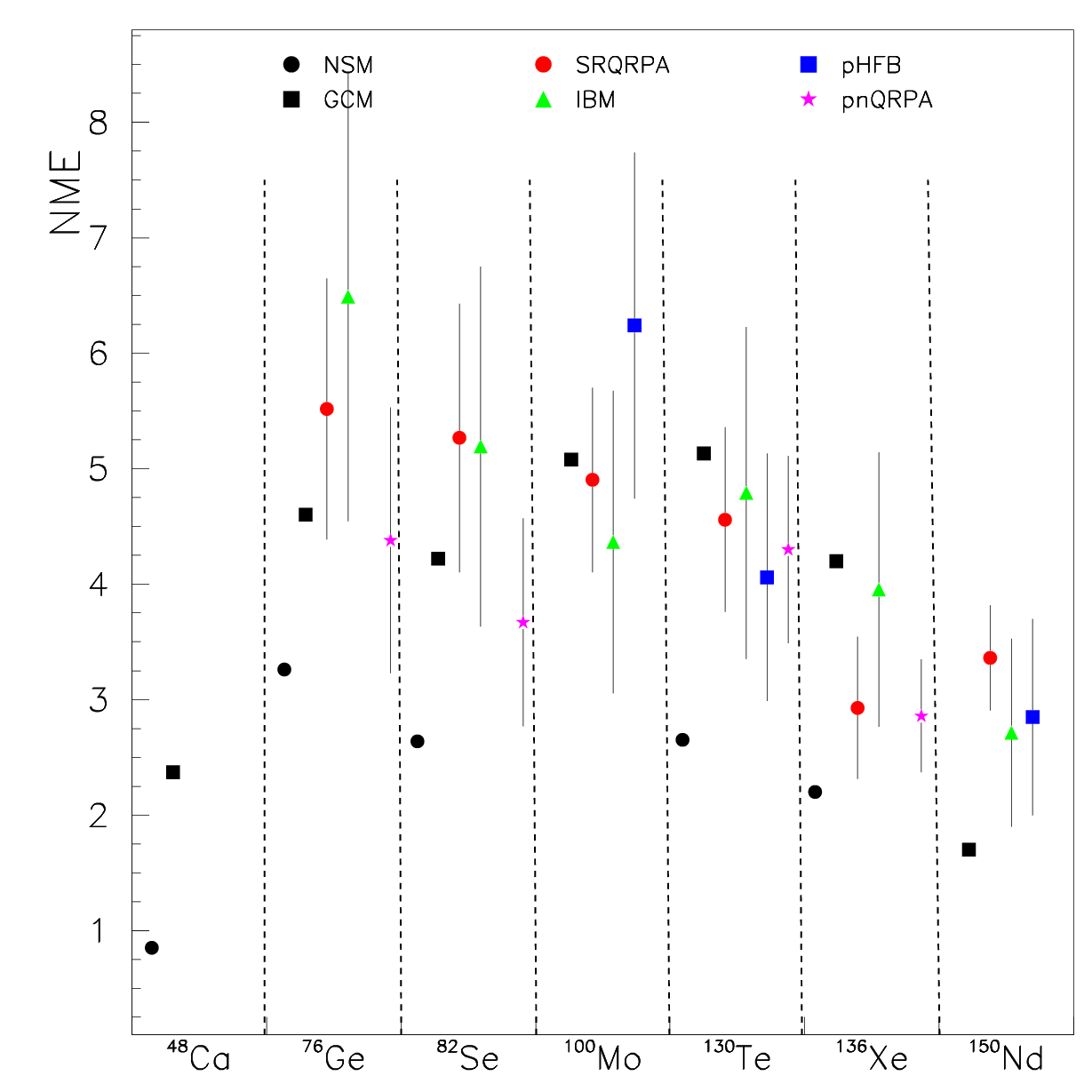
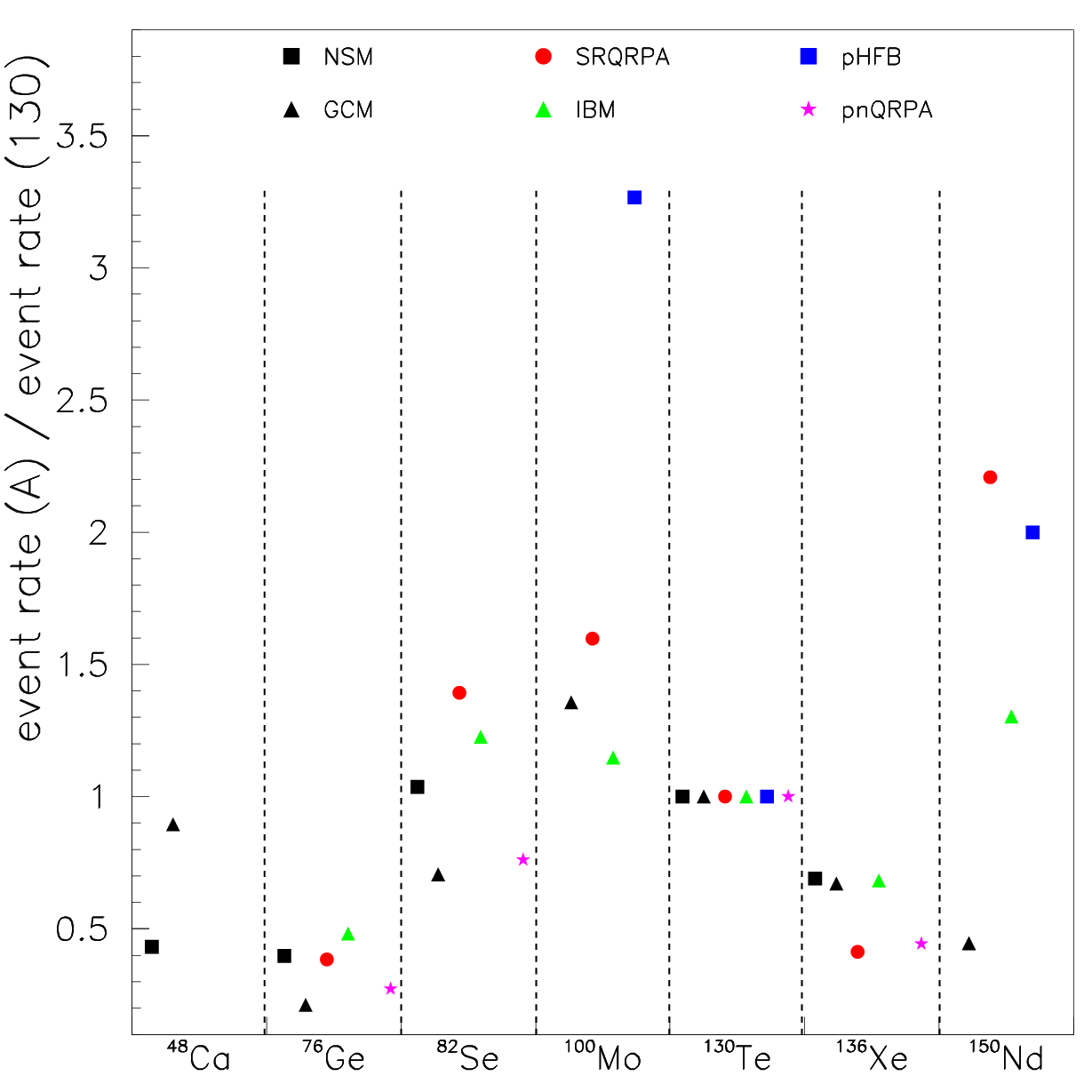
Figure 1: Left: Different calculations for nuclear matrix elements for $0\nu\beta\beta$ decay for light neutrino exchange. NSM = Nuclear shell model [17, 18], SRQRPA = self-consistent renormalized quasi-particle random phase approximation [19, 20, 21] (matrix elements are scaled by 1.14 to compensate for different phase space factors), pnQRPA = proton-neutron quasi particle random phase approximation [22], GCM = generating coordinate method [23], IBM = interacting boson model [24, 25] (matrix elements are scaled by 1.18 to estimate the effect if the UCOM short range correlation instead of the Jastrow type would have been used [8]), pHBF= projected Hartree-Fock-Bogoliubov model [26]. Right: ratio of expected $0\nu\beta\beta$ events per kg target mass for the different models normalized to ¹³⁰Te.

While the observation of $0\nu\beta\beta$ would manifest lepton number violation and the neutrino’s Majorana nature, the underlying physics can only be disclosed if the observed $T_{1/2}^{0\nu}$ for different isotopes and possibly other variables like the angle between the emitted electrons is compared to theory. Consequently, there is a large interest in nuclear matrix element calculations and substantial progress has been made during the last years. Traditionally, nuclear shell model (NSM) and quasi particle random phase approximation (QRPA) calculations have been performed. Recently new approaches like the interacting boson model (IBM), the generating coordinate model (GCM) and the projected Hartree-Fock-Bogoliubov (pHFB) method have been applied. A discussion of these calculations is given in [27].

The results of these calculations are shown in Fig. 1. The following statements can be made concerning the status:

• There is no large variation for the NME between the different isotopes. This might be due to the fact that only neighboring neutrons in a nucleus contribute to the decay [17, 20].

• For the NSM, all values are systematically lower than for other methods. Possible reasons for this effect are discussed in the literature [17, 28].

• The differences between the QRPA calculations of different groups are now quite small.

• For a given isotope the calculations spread by typically a factor of 2, i.e. a factor of 4 for $T_{1/2}^{0\nu}$.

• The role of short range correlations has been studied and the UCOM correction has emerged as standard [29]. Alternatively, a self consistent implementation was first applied to SRQRPA [20] and later to other methods [18, 26] and resulted in small changes.

• Experimental input can have a large shift of the result. For example charge exchange reaction measurements of ¹⁵⁰Nd(³He,t) and ¹⁵⁰Sm(t,³He) [30] result in a quenching factor of 0.75 for the $g_{A}$ coupling and hence a reduction of the matrix element by 25% for ¹⁵⁰Nd [21]. In this calculation, deformation was treated for the first time in a QRPA calculation.

  For ⁷⁶Ge and ⁷⁶Se, the proton and neutron valence orbital occupancies have been measured [31, 32]. If the models are adjusted to reproduce these values, the NSM result increases by 15% [18] while the QRPA results are reduced by about 20% [33, 34]. Hence the difference between NSM and QRPA becomes half as large.

The calculations are performed for the standard light neutrino exchange but results for other mechanisms like SUSY particle exchange are also available [35, 19].

In order to see whether some isotopes are better suited for $0\nu\beta\beta$ decay searches from a theoretical point of view, the number of expected decays per isotope mass can be compared. This value includes the phase space factor, the matrix element and the mass number $A$. For the comparison it is sufficient to look at the ratio of decay rates and in this case, some of the systematic effects of the matrix element calculations cancel since there are typically correlations among the isotopes for a given method. The right hand plot of Fig 1 shows these ratios for the different models normalized to the decay rate of ¹³⁰Te. One sees that ⁷⁶Ge is less favorable. The expected decays per kg vary between 20% and 50% of the rate of ¹³⁰Te. In other words: if all experimental parameters were the same then one would need a factor of $\approx$3 more target mass in a ⁷⁶Ge experiment to have the same sensitivity. In reality this is not the case, i.e. the superior energy resolution of Ge detectors compensates this effect.

5 Comparison of experiments

The experiments searching for $0\nu\beta\beta$ decay use a large variety of detection mechanisms and background reduction methods, see Tab. 2. The current status of almost all of them is described in these proceedings. Therefore a more detailed discussion is omitted here. Instead the key performance numbers are taken for a comparison of the sensitivities of some experiments.

Table 2: Selection of $0\nu\beta\beta$ experiments.

experiment	isotope	mass [kg]	method	location	time	ref.
past experiments
Heidelberg-Ms.	76Ge	11	ionization	LNGS	-2003	[16]
Cuoricino	130Te	11	bolometer	LNGS	-2008	[36]
NEMO-3	100Mo,82Se	7,1	track.+calorim.	Modane	-2011	[37]
current experiments
EXO	136Xe	175	liquid TPC	WIPP	2011-	[15]
Kamland-Zen	136Xe	330	liquid scintil.	Kamioka	2011-	[38]
GERDA-I/II	76Ge	17/35	ionization	LNGS	2011-/13	[39]
CANDLES	48Ca	0.35	scint. crystal	Oto Cosmo	2011-	[40]
funded experiments
NEXT	136Xe	100	gas TPC	Canfrac	2014	[41]
Cuore0/Cuore	130Te	10/200	bolometer	LNGS	2012/14	[42]
Majorana Demo.	76Ge	30	ionization	SUSEL	2014	[43]
SNO+	150Nd	44	liquid scint.	Sudbury	2014	[44]
proposal, proto-typing
SuperNEMO	82Se	7/100-200	track.+calorim.	Modane	2014/-	[45]
Cobra	116Cd		solid TPC	LNGS		[46]
Lucifer	82Se		bolom.+scint.	LNGS		[47]
DCBA/MTD	150Nd	32	tracking			[48]
MOON	82Se,100Mo	30-480	track.+scint.			[49]
XMASS	136Xe		liquid scint.	Kamioka		[50]
AMoRE	100Mo	100	bolom.+scint.	YangYang		[51]
Cd exp.	116Cd		scint.			[52]

Since experiments use different isotopes a relative scaling factor for the different matrix elements and phase spaces has to be applied. This factor can be estimated using Fig. 1. The values used here are $f_{A}({\rm Ge})=0.35$, $f_{A}({\rm Se})=1.1$, $f_{A}({\rm Mo})=1.6$, $f_{A}({\rm Te})=1$, $f_{A}({\rm Xe})=0.55$ and $f_{A}({\rm Nd})=2.2$.

If the number of background events is large, equation 12 can be used to estimate the experimental sensitivity. A relative figure-of-merit can then be defined as

$${\rm FOM}=f_{A}\cdot\epsilon\cdot\eta\cdot\sqrt{\frac{M}{B\cdot\Delta E}}$$ (14)

One can call this the “ultimate” relative sensitivity of an experiment. Tab. 3 lists the performance numbers and the figure-of-merit. For running (and past) experiments like EXO and GERDA-I the current achieved values are used which might improve with time while for the others the anticipated performance numbers are taken.

Alternatively, the (relative) sensitivity vs. time can be estimated from equation 11 by

$$\hat{T}_{1/2}^{0\nu}>\frac{f_{A}\cdot\epsilon\cdot\eta\cdot M\cdot t}{\Psi(B\cdot\Delta E\cdot M\cdot t)}$$ (15)

Here $\Psi(\lambda_{\rm bkg})$ is the “average” 90%C.L. upper limit of the number of signal events for $\lambda_{\rm bkg}$ background events calculated according to the method discussed in [29]. The result is shown in Fig 2. Here all experiments are assumed to start at time 0.

Table 3: Comparison of figure-of-merits (FOM) for the case of large number of background events (“ultimate sensitivity”). $f_{A}$ is the scale factor for a given isotope taken from Fig. 1(right), and $\Delta E$ is the energy window which is taken here to be 1(2) full width half maximum for experiments with $>0.5\%$ ($<0.5\%$) resolution. Note that the efficiency is reduced by 0.7 if $\Delta E=$ 1$\cdot$FHWM. FOM is defined in the text.

experiment	mass	$f_{A}$	background	$\Delta E$	efficiency	enrichment	FOM
	[kg]		[$\frac{{\rm cnt}}{{\rm keV}\cdot{\rm kg}\cdot{\rm y}}$]	[keV]
Hd-Moscow	11	0.35	0.12	8	0.8	0.86	0.8
Cuoricino	41	1	0.16	12	0.9	0.27	1.1
NEMO-3	6.9	1.6	0.002	240	0.18	0.9	1.0
EXO	175	0.55	0.004	260	0.33	0.81	1.9
Kamland-Zen	330	0.55	0.0002	250	0.5	0.9	20
GERDA-I	15	0.35	0.03	10	0.8	0.86	1.7
GERDA-II	30	0.35	0.001	6	0.8	0.88	17
Major.-Dem.	20	0.35	0.001	6	0.9	0.9	16
CUORE	750	1	0.01	10	0.9	0.27	21
SNO+	800	2.2	0.0002	230	0.33	0.056	5.4
NEXT	100	0.55	0.0002	25	0.25	0.9	18
SuperNEMO	100	1.1	0.0002	120	0.3	0.9	19
Lucifer	100	1.1	0.001	10	0.9	0.5	50

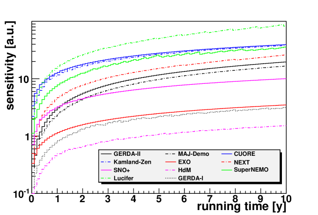
Figure 2: Relative experimental sensitivity for $0\nu\beta\beta$ life time limit versus running time.

A few comments should be made concerning the interpretation of Tab. 3 and Fig. 2.

• If one takes the spread of the data points in Fig. 1 the factor $f_{A}$ has a $\approx 20$% uncertainty.

• The $2\nu\beta\beta$ background is irreducible and can only be avoided with an energy resolution $\sigma<1-2$% at $Q_{\beta\beta}$. This requirement depends of course strongly on $T_{1/2}^{2\nu}$ which varies by a factor of 300 for the isotopes considered. For some experiments this background is not fully taken into account for the background index.

• All sensitivities given are the scales for $0\nu\beta\beta$ discovery. To get relative sensitivities for $m_{\beta\beta}$ the square root has to be taken.

• Of the running experiments, Kamland-Zen should have the largest potential. This is impressive if one takes into account that it was not specially built for this physics.

• Germanium experiments can be very competitive despite the fact that the phase space factor is so small. Especially if a positive signal will be claimed, a narrow peak at $Q_{\beta\beta}$ will be more convincing than a broad shoulder.

• The Lucifer approach with 100 kg is very competitive even in comparison to a ton scale Xe experiment like Kamland-Zen or NEXT.

• Systematic effects like the precision of the energy resolution or the background shape are not taken into account.

In case the neutrino masses are ordered in the inverted mass hierarchy, a lower bound of about 15 meV for $m_{\beta\beta}$ can be calculated using the current parameters from neutrino oscillation experiments. For ⁷⁶Ge this corresponds to half lives of $5-20\cdot 10^{27}$ years. These values should be compared to the expected sensitivity of GERDA-II or the Majorana Demonstrator of about 1.5$\cdot 10^{26}$ y. This demonstrates that exploring the entire mass band of the inverted hierarchy is a long term enterprise. With the numbers in Tab. 3 and a mass of 1000 kg, the required time for $5\cdot 10^{27}$ y is 13 years while a Lucifer like experiment would need to run for half the time.

6 Summary

Neutrinoless double beta decay is the best experimentally accessible method to test whether neutrinos are Majorana particles. This decay violates lepton number and is therefore on equal footing to proton decay searches. The motivation for several large efforts in this field is therefore obvious.

For a long time, the Heidelberg-Moscow experiment has dominated the field and its claim of a $0\nu\beta\beta$ signal has not been scrutinized since 2001. In 2011, EXO, Kamland-Zen, CANDLES and GERDA-I started to take data. All but CANDLES are more sensitive than Heidelberg-Moscow and especially Kamland-Zen is expected to answer this question in the next 12 months. EXO has already reported a first time measurement of $T_{1/2}^{2\nu}(^{136}{\rm Xe})=2.11\pm 0.04({\rm stat})\pm 0.21({\rm syst})\cdot 10^{21}$y which is considerably lower than previous limits [15].

Beyond this next step, experiments want to explore the $m_{\beta\beta}$ region for the inverted neutrino mass hierarchy. This will eventually require ton scale experiments. Which of the proposed solutions will be built is open at the moment.

References

References

- [1] Goeppert-Mayer M 1935 Phys. Rev. 48 512
- [2] Majorana E 1937 Nuovo Cim. 14 171
- [3] Furry W H 1939 Phys. Rev. 56 1184
- [4] Barabash A S 2011 Phys. Atom. Nucl. 74 603 (Preprint arXiv:1104.2714)
- [5] Tretyak V I 2011 conference MEDEX’11, Prague
- [6] Avignone F T, Elliott S R and Engel J 2008 Rev. Mod. Phys. 80 481 (Preprint arXiv:0708:1033)
- [7] Rodejohann W 2011 Int. J. Mod. Phys. E20 1833 (Preprint arXiv:1106.1334)
- [8] Gomez-Cadenas J J et al. 2012 Riv. Nuovo Cim. 35 29 (Preprint arXiv:1109:5515)
- [9] Suhonen J 2011 Phys. Lett. B 701 490 see also talk at TAUP 2011
- [10] Tretyak V 2011 conference TAUP 2011, Munich
- [11] Rukhadze N et al. 2011 Nucl. Phys. A 852 197 see also talk at TAUP 2011
- [12] Danevich F 2011 conference TAUP 2011, Munich, also arXiv:1110.3690
- [13] Nakamura K and others (Particle Data Group) 2010 J. Phys. G 37 075021
- [14] Barabash A S 2010 Phys. Rev. C81 035501 (Preprint arXiv:1003.1005)
- [15] Ackerman N et al. 2011 Phys. Rev. Lett. 107 212501 (Preprint arXiv:1108.4193)
- [16] Klapdor-Kleingrothaus H V et al. 2004 Phys. Lett. B 586 198
- [17] Menendez J et al. 2009 Nucl. Phys. A818 139 (Preprint arXiv:0801.3760)
- [18] Menendez J et al. 2009 Phys. Rev. C80 048501 (Preprint arXiv:0905.1705)
- [19] Faessler A et al. 2011 Phys. Rev. D83 113015 (Preprint arXiv:1103.2504)
- [20] Simkovic F et al. 2009 Phys. Rev. C79 055501 (Preprint arXiv:0902:0331)
- [21] Fang D L et al. 2011 Phys. Rev. C83 034320 (Preprint arXiv:1101:2149)
- [22] Suhonen J and Civitarese O 2010 Nucl. Phys A847 207
- [23] Rodriguez T R and Martinez-Pinedo G 2010 Phys. Rev. Lett. 105 252503 (Preprint arXiv:1008.5260)
- [24] Barea J and Iachello F 2009 Phys. Rev. C79 044301
- [25] Barea J and Iachello F 2011 Nucl. Phys. B (Proc. Suppl.) 217 5
- [26] Rath P K et al. 2010 Phys. Rev. C82 064310 (Preprint arXiv:1104.3965)
- [27] Rodin V 2011 conference TAUP 2011, Munich
- [28] Escuderos A et al. 2010 J. Phys. G37 125108 (Preprint arXiv:1001.3519)
- [29] Gomez-Cadenas J J et al. 2011 JCAP 2011 7 (Preprint arXiv:1010:5112)
- [30] Guess C J et al. 2011 Phys. Rev. C83 064318 (Preprint arXiv:1105.0677)
- [31] Schiffer J P et al. 2008 Phys. Rev. Lett. 100 112501 (Preprint arXiv:0710:0719)
- [32] Kay B P et al. 2009 Phys. Rev. C79 021301 (Preprint arXiv:0810.4108)
- [33] Simkovic F et al. 2009 Phys. Rev. C79 015502 (Preprint arXiv:0812:0348)
- [34] Suhonen J and Civitarese O 2008 Phys. Lett. B668 277
- [35] Hirsch M, Klapdor-Kleingrothaus H V and Kovalenko S G 1998 Phys. Rev. D57 1947 (Preprint arXiv:9707207)
- [36] Andreotti E et al. 2011 Astropart. Phys. 34 822
- [37] Simard L 2011 conference TAUP 2011, Munich
- [38] Kozlov A 2011 conference TAUP 2011, Munich
- [39] Cattadori C 2011 conference TAUP 2011, Munich
- [40] Ogawa I 2011 conference TAUP 2011, Munich
- [41] Capilla F M 2011 conference TAUP 2011, Munich, also arXiv:1106.3630
- [42] Gorla P 2011 conference TAUP 2011, Munich, also arXiv:1109.0494
- [43] Wilkerson J 2011 conference TAUP 2011, Munich, also arXiv:1111.5578
- [44] Hartnell J 2011 conference TAUP 2011, Munich
- [45] Barabash A 2011 conference TAUP 2011, Munich, also arXiv:1112.1784
- [46] Oldorf C 2011 conference TAUP 2011, Munich
- [47] Cardani L 2011 conference TAUP 2011, Munich
- [48] Ishikawa T et al. 2011 Nucl. Inst. Meth. A 628 209
- [49] Fushimi K et al. 2010 J. Phys. Conf. Ser. 203 012064
- [50] Yamashita M (XMASS) 2010 Prepared for 6th Patras Workshop on Axions, WIMPs and WISPs, Zurich, Switzerland, 5-9 Jul 2010
- [51] Kornoukhov V 2011 conference TAUP 2011, Munich
- [52] Barabash A S 2011 JINST 6 P08011 (Preprint arXiv:1108.2771)