Little-used Mathematical Structures
in Quantum Mechanics
II. Representations of the CCR and Superseparability

Abstract

It often goes unnoticed that, even for a finite number of degrees of freedom, the canonical commutation relations have many inequivalent irreducible unitary representations; the free particle and a particle in a box provide examples that are both simple and well-known. The representations are unitarily inequivalent because the spectra of the position and momentum operators are different, and spectra are invariant under unitary transformations. The existence of these representations can have consequences that run from the merely unexpected to the barely conceivable. To start with, states of a single particle that belong to inequivalent representations will always be mutually orthogonal; they will never interfere with each other. This property, called superseparability elsewhere, is well-defined mathematically, but has not yet been observed. This article suggests two single-particle interference experiments that may reveal its existence. The existence of inequivalent irreducibile representations may be traced to the existence of different self-adjoint extensions of symmetric operators on infinite-dimensional Hilbert spaces. Analysis of the underlying mathematics reveals that some of these extensions can be interpreted in terms of topological, geometrical and physical quantities that can be controlled in the laboratory. The tests suggested are based on these interpretations. In conclusion, it is pointed out that mathematically rigorous many-worlds interpretations of quantum mechanics may be possible in a framework that admits superseparability.

1 Introduction: Superseparability

In complete contrast to the representations of Lie groups, representations of the canonical commutation relations (hereafter CCR) for a finite number of degrees of freedom have attracted little attention from physicists. Although uncountably many pairwise-inequivalent irreducible unitary representations (hereafter IURs) of the CCR are routinely constructed in introductory texts on quantum mechanics, they are not given the recognition they deserve, for the mere existence of inequivalent IURs suffices to open the door to new and unexpected phenomena.

In von Neumann’s formulation of quantum mechanics, it is tacitly assumed that the pure states of a single particle always belong to a fixed irreducible unitary representation $\pi$ of the CCR. If this assumption is dropped, then a pure state of a single particle may have components that belong to inequivalent IURs of the CCR. This property has been called superseparability in [14]. In the simplest case, in which only two IURs are admitted, the single-particle Hilbert space will be

$$\mathfrak{H}=\mathfrak{H}_{1}\oplus\mathfrak{H}_{2},$$ (1.1)

where $\mathfrak{H}_{1,2}$ carry inequivalent IURs $\pi_{1,2}$ respectively. The generic single-particle state will be

$$\Psi=\Psi_{1}+\Psi_{2},$$ (1.2)

where

$$\Psi_{1}=\psi_{1}\oplus 0,\;\;\Psi_{2}=0\oplus\psi_{2},\quad\psi_{1}\in\mathfrak{H}_{1}\;\;\text{and}\;\;\psi_{2}\in\mathfrak{H}_{2}.\quad$$ (1.3)

We would then have

$$(\Psi_{1},\Psi_{2})=0\;\,\forall\;\,\psi_{1}\in\pi_{1}\;\text{and}\;\psi_{2}\in\pi_{2},$$ (1.4)

even if $\psi_{1}$ and $\psi_{2}$ have exactly the same dependence on the space coordinates at any given time! Note that, for (1.4) to hold, it is not necessary that $\pi_{1}$ and $\pi_{2}$ be inequivalent.

Is superseparability only a property of the mathematical formalism of quantum mechanics, or is it also reflected in nature? This question can be answered, if at all, only by experiment, and the aim of the present paper is to suggest two single-particle interference experiments that may be performable in the laboratory. The suggestions will based on an analysis of the mathematical conditions that give rise to inequivalent representations.

This analysis requires much more mathematical machinery than the preceding paper [15]. To devise an experiment, one has to identify entities that influence the phenomenon and can be controlled in the laboratory. In the case of superseparability, some of these entities appear to be hidden in the definitions of unbounded self-adjoint operators on a separable Hilbert space. In infinite dimensions the concept of self-adjointness has complexities that do not exist on finite-dimensional vector spaces. Although this concept was analyzed by von Neumann in 1929–30 [17] (and expounded in considerable detail in his book Mathematische Grundlagen der Quantenmechanik in 1932 [19]), only mathematical physicists specializing in functional-analytic methods may be assumed to be familiar with it. Additionally, the problem we wish to address intertwines geometrical questions concerning the relation between Lie groups and Lie algebras with functional-analytic questions concerning the notion of self-adjointness of operators on a separable Hilbert space. The present paper, which is addressed to experimental as well as theoretical physicists, will not assume this mathematical background, and will begin with a concise but adequate account of the material that will be called upon.

Mindful of what was said above, the present paper is organized as follows. Section 2 goes back to where it all began, and describes some work by Hermann Weyl in 1928 and John von Neumann in 1929-30 which set the stage for everything that followed. Apart from its intrinsic interest, the historical background also reveals the geometrical aspect of the problems that we have to address. Then comes the functional-analytic aspect, which is the theory of unbounded symmetric and self-adjoint operators. A brief summary of the material that is essential for our purposes is provided in Sec. 3. Inequivalent representations of the CCR are discussed in Sec. 4. The discussion, aimed at unearthing quantities that can be controlled in the laboratory rather than at mathematical complexities of the subject, is based on three examples: the one mentioned briefly in footnote 2, one due to Schmüdgen and one due to Reeh. Conditions under which superseparability may be revealed in one-particle interference experiments are discussed in Sec. 5. Based on this discussion, two experiments are suggested in Sec. 6: a “2+1-slit” far-field interferometry experiment, and one using Reeh’s observation on the Aharonov-Bohm effect. The concluding section discusses superseparability and the many-worlds interpretation of quantum mechanics.

2 Historical background

We begin by recalling two basic facts. (i) The Born-Jordan commutation relation $[p,q]=-\mathrm{i}\,\!I$ cannot be represented by finite-dimensional matrices if $I$ is required to be the identity matrix. (ii) If it is represented on an infinite-dimensional Hilbert space $\mathfrak{H}$ with $I$ as the identity operator, then at least one of $p$ and $q$ must be represented by an unbounded operator (see, for example, [14]). Recall that an infinite-dimensional Hilbert space is required to be complete, i.e., every Cauchy sequence has to converge, and separable, i.e. has to have a countable orthonormal base. These requirements are automatically satisfied by finite-dimensional Hilbert (or inner product) spaces. All our Hilbert spaces will be over the complex numbers.

Unbounded operators are not defined everywhere on a Hilbert space, and are discontinuous wherever they are defined. They give rise to mathematical phenomena that are not encountered in the theory of finite dimensional matrices, and it requires considerable effort to invest with meaning even the simplest of assertions, such as $[A,B]=0$, if $A$ and $B$ are unbounded. The basic structures of quantum mechanics, namely matrix mechanics, wave mechanics and transformation theory were laid down in 1925–27, but unbounded operators began to be explored only in 1929–1930 [17]. In retrospect, one is struck by the fact that transformation theory could be developed with scant understanding of the operators that were to be transformed. By what magic was this achieved?

In 1928, Weyl published his book Gruppentheorie und Quantenmechanik [20]. In this book he replaced the canonical commutation relations for $N$ degrees of freedom by a $2N$-parameter Lie group, which had the CCR as its Lie algebra; in one fell swoop, he eliminated the vexing problems associated with unbounded operators and brought the subject under the ambit of group theory. This group has become known as the Weyl group, and we shall denote it by $\mathscr{W}_{N}$. We shall give the argument for $N=1$; the general case merely requires a cumbersome modification of the notation (see [20], pp. 272–276).

Let $a,b\in\mathbb{R}$ and define, formally,

$$u(a)=\exp\,(\mathrm{i}ap),\qquad v(b)=\exp\,(\mathrm{i}bq).$$ (2.1)

From the properties of the exponential function, it follows that

$$u(a)u(a^{\prime})=u(a+a^{\prime}),\qquad v(b)v(b^{\prime})=v(b+b^{\prime}).$$ (2.2)

Set $u(0)=v(0)=\mathbf{1}$ and $u(a)^{-1}=u(-a)$, $v(b)^{-1}=v(-b)$. Formal computation yields the result

$$u(a)v(b)u(a)^{-1}v(b)^{-1}=\mathrm{e}^{\mathrm{i}ab}\mathbf{1}.$$ (2.3)

By definition, the Weyl group $\mathscr{W}_{1}$ consists of the elements $\{u(a),v(b)|a,b\in\mathbb{R}\}$, with multiplication defined by (2.2) and (2.3). The element $\mathbf{1}$ is the identity of the group. The group $\mathscr{W}_{1}$ is nonabelian and noncompact, with $\mathbb{R}^{2}$ as the group manifold, and is a Lie group. The same is true of the Weyl group $\mathscr{W}_{N}$ for $N$ degrees of freedom, except that its group manifold is $\mathbb{R}^{2N}$.

Being noncompact, Weyl groups have no finite dimensional unitary representations. In a unitary representation, the elements $u(a)$ and $v(b)$ of $\mathscr{W}_{1}$ are represented by unitary operators $U(a)$ and $V(b)$ on the Hilbert space $\mathfrak{H}$, and similar statements hold for $\mathscr{W}_{N}$. A result known as Stone’s theorem asserts that a one-parameter group of unitaries $\{U(t)\}$ on a Hilbert space has an infinitesimal generator $H$, so that $U(t)=\exp\,(\mathrm{i}Ht)$, where $H$ is self-adjoint. It is bounded if $\{U(t)\}$ is compact ($t\in S_{1}$, the circle) and unbounded if $\{U(t)\}$ is not compact ($t\in\mathbb{R}$). A representation of $\mathscr{W}_{N}$ defines, uniquely, a representation of its Lie algebra – the CCR – by self-adjoint operators. In the representation so defined, the operators $p$ and $q$ are unbounded.

In 1930 von Neumann proved that, for finite $N$, the Weyl group $\mathscr{W}_{N}$ has only one irreducible unitary representation [18]. He gave the name Schrödinger operators to the representatives of the canonical variables $p_{j},q_{j}$, $j=1,\ldots,N$, and titled his paper ‘Die Eindeutigkeit der Schrödingerschen Operatoren’ – Uniqueness of the Schrödinger Operators – a choice that has turned out to be misleading. His result has become known as ‘von Neumann’s uniqueness theorem’ (sometimes as the Stone-von Neumann uniqueness theorem).

A Lie group defines a unique Lie algebra, but the converse is not true. The simplest examples are the covering groups of compact non-simply-connected Lie groups. Examples of this phenomenon that are relevant to elementary particle physics were unearthed as early as 1962 by Michel [8]. The canonical commutation relations are not abstractly equivalent to the Weyl group; as we shall see below, the $p_{j},q_{k}$ will not even generate a Lie group unless they are represented by self-adjoint operators, and the requirement of self-adjointness cannot be met even in simple physical situations (such as spaces with boundaries, cuts or holes) in which $q_{j}$ is the operator of multiplication by $x_{j}$ and $p_{k}=-\mathrm{i}\partial/\partial x_{k}$.

3 Symmetric operators; self-adjointness

Let $\mathfrak{H}$ be a Hilbert space and $A:\mathfrak{H}\rightarrow\mathfrak{H}$ an operator on it. If there exists a positive number $K$ such that $||A\psi||\leq K||\psi||$ for all $\psi\in\mathfrak{H}$, then $A$ is said to be bounded. If no such $K$ exists, then $A$ is said to be unbounded. An unbounded operator $A$ is not defined everywhere on $\mathfrak{H}$; the subset $\mathfrak{D}(A)\subsetneq\mathfrak{H}$ on which it is defined is called the domain of $A$. If $\mathfrak{D}(A)$ is not dense in $\mathfrak{H}$ then $A$ is not yet mathematically manageable, and one generally assumes that $A$ is densely defined, i.e., $\mathfrak{D}(A)$ is dense in $\mathfrak{H}$. (The topology on $\mathfrak{H}$ is the metric topology defined by the metric on $\mathfrak{H}$.)

In the rest of this section we shall deal only with unbounded operators, and therefore the adjective ‘unbounded’ will be omitted.

In operator theory, an operator $A$ is called closed if the set of ordered pairs $\{(\psi;A\psi)|\psi\in\mathfrak{D}(A)\}$ is a closed subset of $\mathfrak{H}\times\mathfrak{H}$. An operator $A_{1}$ is an extension of $A$ if $\mathfrak{D}(A)\subset\mathfrak{D}(A_{1})$ and $A_{1}\psi=A\psi$ for $\psi\in\mathfrak{D}(A)$; one writes $A\subset A_{1}$. An operator is called closable if it has a closed extension. Every closable operator $A$ has a smallest closed extension, which is denoted by $\bar{A}$.

In matrix theory, the adjoint is defined by $(T\boldsymbol{x},\boldsymbol{y})=(\boldsymbol{x},T^{\star}\boldsymbol{y})$. In operator theory, one has to take domains into consideration. Let $\varphi,\xi\in\mathfrak{H}$ such that $(A\psi,\varphi)=(\psi,\xi)$ for all $\psi\in\mathfrak{D}(A)$, and define $A^{\star}$ by $A^{\star}\varphi=\xi$. Then $\mathfrak{D}(A^{\star})$ is precisely the set of these $\varphi$. One can show that if $A$ is densely defined, then $A^{\star}$ is closed. Furthermore, $A^{\star}$ is densely defined if and only if $A$ is closable, and if it is, then $(\bar{A})^{\star}=A^{\star}$.

We now come to the key definitions. If $\mathfrak{D}(A)\subset\mathfrak{D}(A^{*})$ and $A\varphi=A^{*}\varphi$ for all $\varphi\in\mathfrak{D}(A)$, then $A$ is called symmetric. If $\mathfrak{D}(A)=\mathfrak{D}(A^{*})$ and $A\varphi=A^{*}\varphi$ for all $\varphi\in\mathfrak{D}(A)$, then $A$ is called self-adjoint. Self-adjoint operators form a subclass of symmetric operators.

A symmetric operator may have no self-adjoint extension, it may have many self-adjoint extensions, or it may have only one. In the last case, it is called essentially self-adjoint. One can show that if $A$ is essentially self-adjoint, then its closure $\bar{A}$ is self-adjoint, i.e., $\bar{A}$ is the unique self-adjoint extension of $A$.

The fundamental differences between symmetric and self-adjoint operators are:

1. The spectrum of a self-adjoint operator is a subset of the real line, whereas the spectrum of a symmetric operator is a subset of the complex plane; a symmetric operator is self-adjoint if and only if its spectrum is a subset of the real line.

2. A self-adjoint operator can be exponentiated, i.e., if $A$ is self-adjoint then $\exp\,(\mathrm{i}tA)$ is defined for all $t\in\mathbb{R}$; a symmetric operator which is not self-adjoint cannot be exponentiated.

If $A$ and $B$ are self-adjoint, defined on a common dense domain $\mathfrak{D}$ and commute on $\mathfrak{D}$, then $\exp\,(\mathrm{i}aA)$ and $\exp\,(\mathrm{i}bB)$ are defined for all $a,b\in\mathbb{R}$ and commute. However, if $A$ and $B$ are merely essentially self-adjoint, are defined on $\mathfrak{D}$ and commute on $\mathfrak{D}$, then $\exp\,(\mathrm{i}a\bar{A})$ and $\exp\,(\mathrm{i}b\bar{B})$ do not necessarily commute. This fact, which is highly counterintuitive, was unearthed by Nelson in 1958, and is sometimes known as the Nelson phenomenon; for details and references, see Reed and Simon [10, 11].

We shall conclude this section with an example. The group of isometries of $\mathbb{R}^{2}$ consists of translations and rotations. The group of isometries of the punctured plane $\mathbb{R}^{2}\setminus\{O\}$ is the group of rotations about the origin $O$. What happens to the translation operators on $\mathbb{R}^{2}$, namely $\exp\,(\mathrm{i}ap_{x})$ and $\exp\,(\mathrm{i}bp_{y})$, $a,b\in\mathbb{R}$ (where $p_{x}=-\mathrm{i}\partial/{\partial x},\;p_{y}=-\mathrm{i}\partial/{\partial y}$), when the origin is excised?

The operators $\partial/{\partial x},\,\partial/{\partial y}$ are defined on sets of differentiable functions. A function which is differentiable on $\mathbb{R}^{2}$ is necessarily differentiable on $\mathbb{R}^{2}\setminus\{O\}$, but the converse is not true; the latter has a richer supply of differentiable functions than $\mathbb{R}^{2}$, e.g., the function $r^{-1}\exp\,(-r^{2}/2)$ (which is also square-integrable). Excising the origin has, in this case, enlarged the set of differentiable functions on which $p_{x}$ and $p_{y}$ are defined. We state without proof that this enlargement changes the spectra of these operators, which in turn leads to the failure of self-adjointness and exponentiability.

4 Inequivalent representations of the CCR

Inequivalent IURs of the relativity or internal symmetry groups used in physics are completely classified by values of the invariants of their Lie algebras, and these invariants can be determined in the laboratory. By contrast, the only invariant of the Lie algebra defined by the CCR is the identity, and a useful classification of IURs of the CCR is not yet known. If we want to distinguish between inequivalent IURs in the laboratory, then, in the present state of our knowledge, our only option is to examine the mathematical structures that give rise to inequivalent IURs in search of clues. As stated earlier, we shall confine our search to the analysis of specific examples.

4.1 An example from the textbooks

Consider first the free (spinless) particle on the real line. Its Hilbert space is $L^{2}(\mathbb{R},\mathrm{d}x)$. The operators $p$ and $q$ are self-adjoint and are defined on a common dense domain. Their spectra are continuous, and fill the real line. We shall denote this representation of the CCR by $\pi_{\mathbb{R}}$.

Consider now a particle which is constrained to lie in the interval $[0,\Lambda]\subset\mathbb{R}$. Its Hilbert space is the subspace $\mathfrak{H}_{\sf box}$ of $L^{2}([0,\Lambda],\mathrm{d}x)$ consisting of (equivalence classes of) functions that vanish at the boundaries. Denote the representation of the CCR on $\mathfrak{H}_{\sf box}$ by $\pi_{\Lambda}$.

One knows from textbook physics that the spectrum of $p$ in $\mathfrak{H}_{\sf box}$ is discrete; its eigenvalues are $n\pi/\Lambda,n=1,2,\ldots$ (we take $\hbar=1$). This is enough to establish that the representations $\pi_{\mathbb{R}}$ and $\pi_{\Lambda}$ of the CCR for one degree of freedom are unitarily inequivalent to each other, because the spectrum of an operator is invariant under unitary transformations. Furthermore, if $\Lambda^{\prime}$ is such that $\Lambda/\Lambda^{\prime}$ is irrational, then the representations $\pi_{\Lambda}$ and $\pi_{\Lambda^{\prime}}$ are unitarily inequivalent. Since there are infinitely many real numbers such that the quotient of any two of them is irrational, this example gives us infinitely many pairwise inequivalent IURs of the CCR for one degree of freedom. Note that the operators $p$ on the concrete Hilbert spaces $\mathfrak{H}_{\sf box}$ are determined by the boundary conditions at the ends of the intervals $[0,\Lambda]$.

These examples extend immediately to higher dimensions.

4.2 An example due to Schmüdgen

The example given below is Example 1 of §3 in [13]. We shall omit all computations and proofs.

Let $\mathfrak{H}=L^{2}(\mathbb{R}^{2})$ and $\varphi\in\mathfrak{H}$. Let $z$ be a complex number such that $|z|=1$ but $z\neq 1$. Define the unitary operators $U(t),V(s)$ by

$$\begin{array}[]{lcl}(U(t)\varphi)(x,y)&=&\mathrm{e}^{\mathrm{i}zx}\varphi(x,y+t),\quad t\in\mathbb{R}\\[5.69054pt] (V(s)\varphi)(x,y)&=&\left\{\begin{array}[]{rcl}\varphi(x+s,y)&\text{for}&y>0,x\geq 0\\ &&\text{and}\quad y>0,x+s<0\\[2.84526pt] z\varphi(x+s,y)&\text{for}&y>0,x<0\\ &&\text{and}\quad x+s\geq 0\\[2.84526pt] \varphi(x+s,y)&\text{for}&y\leq 0,x\in\mathbb{R}\end{array}\right.\end{array}$$ (4.1)

for $s>0$, and similarly for $s<0$. The operator $V(s)$ is a translation in the $x$-direction, with a certain modification: in the lower half-plane (including the $x$-axis), it takes $\varphi(x,y)$ to $\varphi(x+s,y)$, but, in the open upper half-plane, it multiplies the translated function $\varphi(x+s,y)$ by $z$ whenever the $y$-axis is crossed.

The sets $\{U(t)|t\in\mathbb{R}\}$ and $\{V(s)|s\in\mathbb{R}\}$ define two one-parameter groups. Their infinitesimal generators are given by

$$Q=x-\mathrm{i}\frac{\partial}{\partial y}\quad\text{and}\quad P=-\mathrm{i}\frac{\partial}{\partial x}\cdot$$ (4.2)

Formally, $[Q,P]=\mathrm{i}I$. Let now $\mathscr{R}(s,t)=\{(x,y)|0<x\leq s,0<y\leq t\}$, and denote by $\chi^{\mathscr{R}(s,t)}$ the characteristic function of $\mathscr{R}(s,t)$, i.e.,

$$\chi^{\mathscr{R}(s,t)}=\left\{\begin{array}[]{ll}1,&(x,y)\in{\mathscr{R}(s,t)}\\[5.69054pt] 0,&(x,y)\notin{\mathscr{R}(s,t)}.\end{array}\right.$$

Then, for $\varphi\in\mathfrak{H}$,

$$(I-\mathrm{e}^{-\mathrm{i}ts}V(-s)U(-t)V(s)U(t))\varphi=(1-z)\chi^{\mathscr{R}(s,t)}\varphi$$ (4.3)

Since $z\neq 1$, (4.3) shows that the $U(s)$ and $V(t)$ do not satisfy the relations (2.3) that define the Weyl group. The representation $\pi_{S}$ of the CCR for one degree of freedom determined by (4.1) turns out to be irreducible; it is clearly not equivalent to the representation $\pi_{\mathbb{R}}$.

There exist many examples of inequivalent irreducible representations of the CCR $[Q,P]=\mathrm{i}I$ in which $P$ and $Q$, defined on functions that are themselves defined on various two-dimensional spaces, have the form (4.2) or forms similar to it; we refer the reader to [13] for details, and for references to earlier works. As we have not found a way to relate these $P,Q$ to the degrees of freedom of a physical system, we shall not dwell on these representations.

4.3 Reeh’s example

In 1988, Helmut Reeh showed that that the Nelson phenomenon could be found in the Aharonov-Bohm effect [12]. The motion of a spinless particle of charge $q$ in a plane perpendicular to a magnetic flux trapped along the $z$-axis is two-dimensional. Its canonical operators may be written, formally, as

$$\boldsymbol{p}=-\mathrm{i}\frac{\partial}{\partial\boldsymbol{x}}+q\boldsymbol{A},\;\;\boldsymbol{q}=\text{multiplication by}\;\boldsymbol{x}.$$ (4.4)

Boldface symbols denote 2-vectors in the $XY$-plane. The vector potential $\boldsymbol{A}$ (up to a gauge) can be written, in terms of the magnetic flux $\Phi$, as

$$\boldsymbol{A}=\frac{\Phi}{2\pi r}\boldsymbol{e},$$ (4.5)

where $r=(x^{2}+y^{2})^{1/2}$ and $\boldsymbol{e}$ is the unit vector at $(x,y)$ tangent to the circle $r=\text{const}$:

$$\boldsymbol{e}=\left(-\frac{y}{r}\raisebox{2.15277pt}{,}{}\;\frac{x}{r}\right)\cdot$$

We shall set

$$\alpha=\frac{q{\Phi}}{{2\pi}}$$ (4.6)

and use (4.5) to rewrite the quantities $\boldsymbol{p}$ of (4.4) as

$$\boldsymbol{p}^{\alpha}=-\mathrm{i}\frac{\partial}{\partial\boldsymbol{x}}+\alpha\frac{\boldsymbol{e}}{r},$$ (4.7)

where the $\alpha$-dependence of $\boldsymbol{p}$ has been rendered explicit on the left. The problem is to define the formal quantities $p_{x}^{\alpha}$ and $p_{y}^{\alpha}$ in (4.7) as operators on the Hilbert space $L^{2}(\mathbb{R}^{2}\setminus O)=L^{2}(\mathbb{R}^{2})$; excision of a single point, here the origin $O$, has no real effect on an $L^{2}$-space, but – as we have seen earlier – changing the domains of differentiation operators ever so slightly can have drastic consequences. Reeh chose, for the common domain of $p_{x}^{\alpha},\,p_{y}^{\alpha}$, the space $\mathscr{D}(\mathbb{R}^{2}\setminus O)$ of smooth functions with compact support on $\mathbb{R}^{2}\setminus O$. The space $\mathscr{D}(\mathbb{R}^{2}\setminus O)$ is dense in $L^{2}(\mathbb{R}^{2})$, and $p_{x}^{\alpha}$ and $p_{y}^{\alpha}$ are operator-valued distributions on it. If $\varphi\in\mathscr{D}(\mathbb{R}^{2}\setminus O)$, then it follows from $\text{curl}\,\boldsymbol{A}=0$ that $[p_{x}^{\alpha},\,p_{y}^{\alpha}]\varphi=0$.

Consider now the equation

$${p}^{\alpha}_{x}\varphi=\left(-\mathrm{i}\frac{\partial}{\partial x}-\alpha\frac{y}{x^{2}+y^{2}}\right)\varphi=\lambda\varphi.$$ (4.8)

It is a linear homogeneous differential equation of the first order which can be solved explicitly for any $\lambda\in\mathbb{C}$, and the same holds for the equation ${p}_{y}^{\alpha}\psi=\lambda\psi$. The solutions do not have compact support. By exploiting these solutions, Reeh established the following results [12]:

1. The operators $p_{x}^{\alpha}$ and $p_{y}^{\alpha}$ are not self-adjoint; they are essentially self-adjoint.

2. Let $\bar{p}_{x}^{\alpha}$ and $\bar{p}_{y}^{\alpha}$ be their self-adjoint extensions, and define

   $$V_{x}^{\alpha}(a)=\exp\,(\mathrm{i}a\bar{p}_{x}^{\alpha}),\qquad V_{y}^{\alpha}(b)=\exp\,(\mathrm{i}b\bar{p}_{y}^{\alpha}).$$

   Reeh showed that

   $$V_{x}^{\alpha}(a)V_{y}^{\alpha}(b)V_{x}^{\alpha}(a)^{-1}V_{y}^{\alpha}(b)^{-1}=\mathrm{e}^{\mathrm{i}(\pi\alpha/2)\cdot[\epsilon(x)-\epsilon(x+a)][\epsilon(y)-\epsilon(y-b)]}\,I,$$ (4.9)

   where $I$ is the identity operator, and

   $$\epsilon(t)=\left\{\begin{array}[]{rl}1&\;\;t>1\\[5.69054pt] -1&\;\;t<1.\end{array}\right.$$

Note that the product $[\ldots][\ldots]$ in the exponent on the right-hand side of (4.9) can only assume the values $0,\pm 4$, so that the entire right-hand side can only assume the values $I,\exp\,(\pm 2\pi\mathrm{i}\alpha)I$. It follows that if $\alpha$ is an integer, then the right-hand side of (4.9) equals the identity operator $I$ for all admissible $x,y,a,b$, but not if $\alpha$ is not an integer; in this case the group generated by the operators $\{x,y,\bar{p}_{x}^{\alpha},\bar{p}_{y}^{\alpha}\}$ is no longer isomorphic with the Weyl group $W_{2}$. Clearly, the groups generated by these operators for $\alpha=\alpha_{1},\alpha_{2}$ are not isomorphic with each other if $\alpha_{1}-\alpha_{2}$ is not an integer, and therefore the representations of the CCR (for two degrees of freedom) they define are not unitarily equivalent.

Suppose now that the flux $\Phi$ is trapped inside a superconducting cylinder. It must then be an integral multiple of $\pi/e$, where $e$ is the electronic charge. Substituting $\Phi=n\pi/e$ in (4.6) and setting $q=e$, we find that $\alpha=n/2$. That is, if the trapped flux consists of an even number of flux quanta, the right-hand side of (4.9) will reduce to $I$, and the group of the CCR to $\mathscr{W}_{2}$. This will not happen if the trapped flux contains an odd number of flux quanta.

5 Controlling representations of the CCR

The preceding discussion has revealed several factors that appear to affect the representation of the CCR and can be manipulated by the experimentalist. They are:

1. Topology of the single-particle configuration space (last two paragraphs of Sec. 3).

2. Geometry of the single-particle configuration space, if the latter is compact (Sec. 4.1).

3. The vector potential, if the single-particle configuration space is not simply connected and the particle is charged.

In the following, we shall suggest two single-particle interference experiments with interferometers that have two asymmetric arms. In the first of these, the asymmetry is topological (as well as geometrical); the exit from one arm is through a single slit, and from the other arm through a double slit. The suggestion is based on the assumption that the representation of the outgoing wave is determined by the configuration space available to it, and will therefore be different for the two arms. The second is based on the assumption that the two arms can be magnetically shielded from each other. Then the interferometer can be so configured that one arm contains a solenoid whereas the other does not, and, from Reeh’s results, the outgoing waves from the different arms will generally be in inequivalent representations.

In these experiments, superseparability will be revealed by a major change in the interference pattern from the one that would be observed in its absence.

6 Suggested experiments

6.1 A 2+1-slit far-field I-D experiment

The device used for the experiment described below will be called a $2+1$-slit interferometer. The interference-diffraction (hereafter I-D) pattern produced by it will depend on the presence or absence of superseparability. If superseparability is absent, the I-D pattern will be the same as that produced by a triple-slit interferometer. That being the case, in the following the phrase ‘$2+1$-slit I-D pattern’ will imply the presence of superseparability. We begin by describing the device.

                ........................................................................................................................................................................................................................................................................................................................................................................................................................................................................$W$$C^{(1)}$$C^{(2)}$$P$$\theta$$b$$s$$x$$O^{(3)}$$O^{(2)}$$O^{(1)}$

Figure 1: Interferometer for $(2+1)$-slit experiment

A cross-section of the $2+1$-slit wavefront-division interferometer is shown in Fig. 1. The partition $W$ separates the chambers $C^{(1)}$ and $C^{(2)}$, which are topologically identical except for the fact that $C^{(1)}$ has only one exit slit whereas $C^{(2)}$ has two. The triple-slit interferometer $C^{(3)}$ is exactly the same as the above, but without the partition $W$. All devices have the same slit width $b$ and the same slit separation $s$.

The partition $W$ will divide the incoming wave into two. One of them will pass through the double slit, but not the single slit; the other will pass through the single slit, but not the double slit. The experiment is based on the assumption that, as a result, the outgoing waves that emerge from $C^{(1)}$ and $C^{(2)}$ will be in inequivalent representations of the CCR. (In the absence of superseparability, the presence or absence of the partition should make little difference to the observed I-D pattern.)

The source is not shown in the figure. It is assumed that the incoming wave, travelling in the direction of the arrows, can be approximated by a plane wave inside the interferometer. The wavelength will be denoted by $\lambda$. The detector is assumed to be distant enough for observing far-field interference effects. In this case we may base our theoretical discussion on the standard formulae for Fraunhofer diffraction.

We shall have to consider three I-D patterns: single-, double- and triple-slit. The centre of a slit system (in the plane of the paper) will be denoted by $O^{(1)},O^{(2)},O^{(3)}$ respectively for the single-, double- and triple-slit systems, as shown in Fig. 1. The angle between the line of sight $OP$ and the outward normal to the interferometer at $O$ will be denoted by $\theta$ for all cases.

The intensity at $P$ for an $N$-slit diffraction grating is given by the formula

$$I(P)=A\left(\frac{b}{x}\right)^{2}\cdot\frac{\sin^{2}\beta}{\beta^{2}}\cdot\frac{\sin^{2}N\gamma}{\sin^{2}\gamma}\raisebox{2.15277pt}{,}$$ (6.1)

where $A$ is a positive constant, $b$ the slit width, $x$ the distance between the interferometer and the detector, $P$ and $\theta$ are as shown in Fig. 1, and $\beta$ and $\gamma$ are defined by

$$\beta=\frac{b}{\lambda}{\pi\sin\theta}\quad\text{and}\quad\gamma=\frac{s+b}{\lambda}{\pi\sin\theta}.$$ (6.2)

In the above, $s$ is the slit separation, as shown in Fig. 1. For a single slit, the interference factor $\sin^{2}N\gamma/\sin^{2}\gamma=1$. For $N=2$ it reduces to $\cos^{2}\gamma$, and for $N=3$, to $(3-4\sin^{2}\gamma)^{2}$. Formula (6.1) is derived in most textbooks on physical optics, for example [6].

                ............................................................................................................................................................................................................................................................................................................................................................................................................................................................................................................................................................................................................................................................................$P^{(2)}_{L}$$P^{(2)}_{U}=P^{(1)}_{L}$................................................................................................................................................................................................................................................................................................................................................................................................................................................................................................................................................................................................................................................................................................................................................................................................................................................................................................................................................................................................................................................................................................................................................................................................................................................................................................................................................$P^{(1)}_{U}$.......................................................................................................................................................................................................................................................................................................................................................................................................................................................................................................................................................................................................................................................................................................................................................................................................................................................................................................................................................................................................................................................................................................................................................................................................................................................................................................................................$W$$C^{(2)}$$C^{(1)}$$Q^{(1)}$$Q^{(2)}$

Figure 2: Central maxima and first diffraction minima

The maxima of the diffraction factor $\sin^{2}\beta/\beta^{2}$ in (6.1) occur at $\tan\beta=\beta$, with the central maximum at $\beta=0$. Its minima (zeroes) occur at $\beta=n\pi,n\neq 0$, with the first minima at $\beta=\pm\pi$. Figure 2 – not drawn to scale – shows the positions of the central maxima and the first diffraction minima at the detection screen for $C^{(1)}$, $C^{(2)}$ and $C^{(3)}$. The central maxima are labelled by $Q$ and the first diffraction minima by $P$. The superscript indicates the number of slits. For the diffraction minima, the subscripts $U,L$ denote upper and lower respectively. The coincidence of $P^{(2)}_{U}$ and $P^{(1)}_{L}$ results from a choice of parameters that will be explained below. The dotted lines in the diagram indicate the diffraction cone for $C^{(3)}$, but, to avoid crowding, the labels $P^{(3)}_{L},\;P^{(3)}_{U},\;Q^{(3)}$ are not shown. Distances $d(A,B)$ between the points $A,B$ are as follows:

$$\delta=d(Q^{(1)},Q^{(2)})=\frac{3}{2}\cdot(s+b)=d(P^{(i)}_{L},P^{(i)}_{U}),\;\;i=1,2,3.$$ (6.3)

From (6.2) we see that for $N$-slit gratings ($N>1$) the slit separation $s$ has no effect on the distances between the diffraction minima, which are determined by the ratio $b/\lambda$ and the angle $\theta$. What the slit separation does affect is the number of interference maxima between two diffraction minima. Let $s=nb$. Then, in the double-slit pattern, there are $n-1$ interference maxima between the central maximum of the intensity and the first diffraction minimum on either side of it. In the triple-slit pattern, there are twice as many, but every other maximum is a secondary maximum, its intensity being roughly 11% of the intensities of the adjacent maxima. In the case of superseparability the amplitudes from $C^{(1)}$ and $C^{(2)}$ will not be added, but the intensities will. In the absence of superseparability the I-D pattern from $C^{(1)}+C^{(2)}$ will be the same as that from $C^{(3)}$.

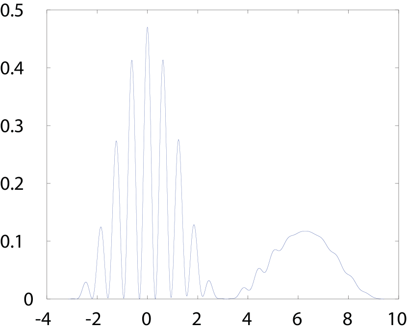
Figure 3: 2+1-slit pattern

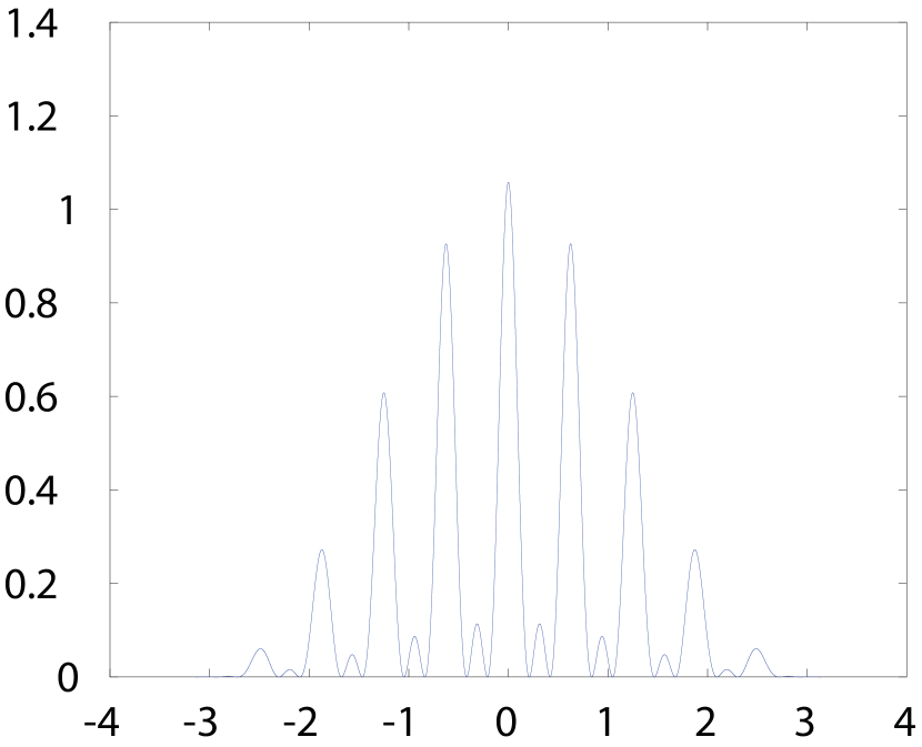
Figure 4: Triple-slit pattern

Figures 4 and 4 show the theoretical intensity plots from the $2+1$-slit ($-\pi\leq\beta\leq 3\pi$) and triple slit ($-\pi\leq\beta\leq\pi)$ interferometers, based on a set of parameters that will be discussed below. The graphs depict the I-D patterns that result when the number of counts from the single slit is half that from the double slit, and the number of counts from the triple slit equals that from the $2+1$-slit.

We shall call the envelopes of the interference patterns from the double and triple slits the diffraction patterns. For the single slit, there is no interference pattern, only a diffraction pattern. In figures 4 and 4, the interference maxima are clearly resolved, because $s/b=5$ is small. Were $s/b$ to be much larger, it would be impossible to resolve the interference maxima, but the $2+1$-slit pattern would continue to exhibit two clearly distinct diffraction maxima, whereas the triple-slit pattern would show only a single diffraction maximum.

Figures 4 and 4 are based on some of the parameters of the interferometry experiment with ⁸⁵Rb atoms reported by Dürr, Nonn and Rempe in [4]. These authors were able to resolve, very clearly, about four peaks per millimeter at the detector. The atoms of ⁸⁵Rb were moving at about 2m/sec, which translates to a wavelength of about $23$nm (nanometre). The parameters assumed for the plots of Figures 4 and 4 are as follows:

1. Wavelength $\lambda=100\text{nm}=10^{-4}\text{mm}$, corresponding to a velocity of 0.5m/sec for ⁸⁵Rb atoms.

2. Slit width $b=0.2\text{mm}$, so that $b/\lambda=2\times 10^{3}$.

3. Slit separation $s=1.0\text{mm}$.

Then from $\beta=(b/\lambda)\pi\sin\theta$ it follows that $\beta=\pm\pi\;\text{for}\;(2\times 10^{3})\sin\theta=\pm 1$. In this case $\sin\theta\approx\theta$ is an excellent approximation, and we find that for $\beta=\pi$, $\theta=\theta_{0}=5\times 10^{-4}$. Furthermore, we see from (6.3) and Fig. 2 that

$$\frac{x}{\delta/2}=\tan\theta_{0}\approx\sin\theta_{0}=\frac{b}{\lambda},$$

and from (6.3) we obtain $x=3b(s+b)/4\lambda$. Using the chosen values of $b,s$ and $\lambda$, we find that $x=1.8$m.

The quantity $\delta=3(s+b)/2=d(Q^{(1)},Q^{(2)})$ is the distance between the centres of the single-slit and double-slit systems in the interferometer. That is, if $x=1.8$m, Fig. 2 provides a faithful representation of the positions of the first diffraction minima at the detection screen. Figure 4 shows the $2+1$-slit intensity pattern on the detection screen between the points $P^{(2)}_{L},P^{(1)}_{U}$, and Fig. 4 the triple-slit pattern between the points $P^{(3)}_{L},P^{(3)}_{U}$ of Fig. 2. The detector used by Dürr, Nonn and Rempe should be able to resolve the interference maxima both in the double-slit and the triple-slit patterns.

6.1.1 Questions of feasibility

The experiment suggested above can, in principle, be carried out with photons, electrons, neutrons, atoms of different elements and even fullerene molecules – practically anything that has been used in an interferometric experiment. The major constraints appear to be:

1. Fabricating the $2+1$-slit interferometer. The slit separation $s$ places an upper limit on the thickness of the partitioning wall $W$. The value of $s$ chosen above was $1$mm, or, or $1000$ microns. The thickness of household aluminium foil is 8–25 microns, so that there is room for improvement here. On the other hand, the distance $\delta$ between the diffraction peaks is $\delta=3(s+b)/2$, so that decreasing $s$ will demand a proportional increase in detector sensetivity.

2. Monochromaticity of the incoming wave. This may be the dominant constraint. In a demonstration experiment with a sodium vapour lamp and a diffraction grating, $b/\lambda$ may be about $2\times 10^{-3}$, or even less. By contrast, with the parameters chosen above, $b/\lambda=2\times 10^{3}$, a difference of six orders of magnitude. In order to observe the interference effects shown in Fig. 4 and Fig. 4, the incoming beam will probably have to be monochromatic over the entire slit system. The magneto-optical trap used by Dürr, Nonn and Rempe as their source may have to be augmented by a suitable monochromator, which will result in a loss of beam intensity.

3. Small wavelength. The wavelength $\lambda$ may be increased by using ultracold atoms, at the cost of reducing the count rate. Using lighter atoms such as ¹²C rather than ⁸⁵Rb would produce a seven-fold increase in the wavelength for the same count rate. Apart from affecting the count rate, increasing the wavelength has the same effect as decreasing the slit width. For the same speed, the wavelength of an electron will be $\approx 1.56\times 10^{4}$ times the wavelength of an ⁸⁵Rb atom.

4. Detector resolution. A tenfold increase in detector resolution will allow $s$ and $b$ to be reduced by factors of 10. For the same $\lambda$, $\theta_{0}$ will increase to $5\times 10^{-3}$, $\sin\theta_{0}\approx\theta_{0}$ will still be true, and $x$ will be reduced by a factor of 10, to 18cm.

To sum up, it would appear that an experiment such as the one suggested above is not unfeasible. An experiment with photons may be the easiest, but for the mathematically-minded theorist photons may be the hardest objects to understand.

Near-field effects depending on Fresnel diffraction or Talbot’s bands may offer other possibilities for the observation of superseparability, but they require separate analysis, and have not been considered here.

6.2 An experiment based on Reeh’s example

The experiment suggested below, based on Reeh’s example, is a single-particle interference experiment with charged particles (typically electrons). The scheme of the experiment is shown in Fig. 5. The source $P$ is far away. $C_{0}$ and $C_{\Sigma}$ are two chambers separated by a wall; they form the arms of the interferometer. $\Sigma$ is a long thin solenoid, perpendicular to the plane of the paper. The current through it is controlled by the experimentalist. The configuration should be such that clearly discernible interference fringes build up at the detector $D$ when there is no current through the solenoid. However, when a current is flowing through the solenoid then, if the phenomenon of superseparability exists, the interference pattern should disappear, to be replaced by two separate diffraction peaks.

                    .......................................................................................................................................................................................................................................................................................................................................................................................................................................................................................................................................$P$$\Sigma$$S_{\Sigma}$$S_{0}$$C_{\Sigma}$$C_{0}$$D$

Figure 5: Interference experiment based on Reeh’s example

From the remarks at the end of Sec. 4.3, one sees that the experiment can also be performed with a superconducting solenoid, provided that the trapped flux is an odd multiple of the flux quantum.

The experiment is based on the assumption that waves emerging from the slits $S_{\Sigma}$ and $S_{0}$ belong to inequivalent irreducible representations of the CCR. The solenoid $\Sigma$ is assumed to control the representation of the wave emerging from the slit $S_{\Sigma}$, and, at the same time, to have no effect on the representation of the one emerging from the slit $S_{0}$. Therefore the first question we have to ask is the following: what are the conditions under which the latter assumption may be valid?

The assumption will be valid if the vector potential due to the solenoid is ‘confined’ to the chamber $C_{\Sigma}$. The fact that a material can confine magnetic fields does not imply that it can also confine vector potentials that cannot be gauged away.

Suppose now that an experiment is performed with the apparatus shown in Fig. 5 (in which the path taken by the wave forms a loop around the solenoid). Then, if the wall separating the chambers $C_{0}$ and $C_{\Sigma}$ were not present, the experiment would simply be one to detect the magnetic Aharonov-Bohm effect. If the configuration shown in Fig. 5 does confine the vector potential due to the solenoid to $C_{\Sigma}$, then the wave through $C_{0}$ would not suffer a phase shift. Therefore, if the influence of stray fields is small, this experiment can have three results:

1. Superseparability is detected.

2. Superseparability is not detected; the interference pattern shows the fringe shift to be expected from the Aharonov-Bohm effect.

3. Superseparability is not detected; the interference pattern shows half the fringe shift to be expected from the Aharonov-Bohm effect.

If superseparability is detected, it would imply that the material which confines the magnetic field also confines the vector potential. If superseparability is not detected and the full Aharonov-Bohm phase shift is observed, it would imply that the vector potential cannot be confined by the material that confines the fields – the experiment is incapable of detecting superseparability. But, if a fringe shift is observed which is only half of what would be expected from the Aharonov-Bohm effect, it would imply that (a) the material does confine the vector potential, and therefore (b) the phenomenon of superseparability does not exist under the given conditions.

Since the chambers $C_{0}$ and $C_{\Sigma}$ cannot be completely closed – each will have an entrance and an exit – the question of stray fields, which was raised to cast doubts on the results of early experiments on the Aharonov-Bohm effect, may be raised again. In retrospect one sees that the effect was clearly observed, most particularly by Möllensted and Bayh, well before the definitive experiment by Tonomura. For details, the reader is referred to the monograph by Peshkin and Tonomura [9]. We therefore believe that in the experiment suggested above, the effect of stray fields will be negligible. However, in view of the smallness of the flux quantum, it may be necessary to shield the apparatus from the earth’s magnetic field.

7 Superseparability and many worlds

If single-particle states can exist in inequivalent IURs of the CCR, it would be natural to ask how states in inequivalent IURs interact with each other. One unexpected possibility will be briefly discussed in the following.

Consider the single-particle Hilbert space $\mathfrak{H}=\mathfrak{H}_{1}\oplus\mathfrak{H}_{2}$ of Sec. 1. Denote by $\mathscr{O}_{\sf max}$ the set of all self-adjoint operators on $\mathfrak{H}$. This set contains operators $O$ such that the matrix element $(\Psi_{1},O\Psi_{2})\neq 0$, where $\Psi_{1,2}$ are defined by (1.3); the particle appears to be changing representations, from $\pi_{1}$ to $\pi_{2}$ and back, due to self-interaction. It is evident that the subset $\mathscr{O}_{\sf min}\subset\mathscr{O}_{\sf max}$ defined by $\mathscr{O}_{\sf min}=\{A_{1}\oplus A_{2}\}$, where $A_{1,2}$ are self-adjoint operators on $\mathfrak{H}_{1,2}$ respectively, does not contain any self-interaction operator. Therefore excluding such self-interactions is equivalent to taking out of consideration the self-adjoint operators in the difference set $\mathscr{O}_{\sf max}\setminus\mathscr{O}_{\sf min}$.

Consider now a two-particle system in the presence of superseparability. Let $\mathfrak{H}=\mathfrak{H}_{1}\otimes\mathfrak{H}_{2}$ be a Hilbert space which carries the representation $\pi_{1}\otimes\pi_{2}$, where $\pi_{1,2}$ are inequivalent IURs of the CCR. One would like to identify the set of admissible interaction operators on $\mathfrak{H}$. At one extreme is the set $\mathscr{C}_{\sf max}$ of all self-adjoint operators on $\mathfrak{H}$. In the absence of restrictions other than self-adjointness on a Hilbert space carrying a single IUR, the other extreme would appear to be the set

$$\mathscr{C}_{\sf min}=\{A_{1}\otimes A_{2}\,|\,A_{k}\;\text{self-adjoint on}\;\mathfrak{H}_{k},\;k=1,2\}.$$ (7.1)

The set (7.1) clearly excludes all operators that can mediate a quantum-mechanical interaction between particles belonging to IURs $\pi_{1}$ and $\pi_{2}$ that are not equivalent to each other. It is as if inequivalent IURs describe different quantum-mechanical worlds. Note that the two particles can still interact classically with each other! Note also that the inequivalence of $\pi_{1}$ and $\pi_{2}$ is crucial; if $\pi_{1}=\pi_{2}$, then the admissible set cannot be $\mathscr{C}_{\sf min}$; it has to be a set $\mathscr{C}$ such that $\mathscr{C}_{\sf max}\supset\mathscr{C}\supsetneq\mathscr{C}_{\sf min}$.

We shall not speculate any further, except for pointing out one intriguing possibility: the existence of inequivalent irreducible representations of the CCR may allow a mathematically rigorous formulation of the many-worlds interpretation of quantum mechanics.

Acknowledgements The author would like to thank Professor H Roos for his comments on an earlier version of this article, and Dr M Goldberg for preparing Figs. 4 and 4.

References

- [1]
- [2]
- [3] Dirac, P A M (1958). The Principles of Quantum Mechanics, Fourth edition (Oxford: The Clarendon Press). First edition, 1930.
- [4] Dürr, S, Nonn, T and Rempe, G (1998). Origin of quantum-mechanical complementarity probed by a ‘which-way’ experiment in an atom interferometer, Nature, 395, 33–37.
- [5] Heisenberg, W (1930). The Physical Principles of Quantum Theory (Chicago: University of Chicago Press). English translation of Die physikalischen Prinzipien der Quantenmechanik, 1930 (Leipzig: Hirzel-Verlag).
- [6] Jenkins, F A and White, H E (1957). Principles of Optics, 3rd ed (New York: McGraw-Hill).
- [7] Mackey, G W (1968). Induced Representations of Groups and Quantum Mechanics (New York-Torino: W A Benjamin-Editore Boringhieri).
- [8] Michel, L (1964). Invariance in quantum mechanics and group extension, in Group-Theoretical Concepts and Methods in Elementary Particle Physics, Lectures of the Istanbul Summer School of Theoretical Physics 1962, Ed F Gürsey (New York: Gordon and Breach) pp 135-200.
- [9] Peshkin, M and Tonomura, A (1989). The Aharonov-Bohm Effect (Berlin: Springer-Verlag) Lecture Notes in Physics Vol 340.
- [10] Reed, M and Simon, B (1972). Methods of Modern Mathematical Physics I Functional Analysis (New York: Academic Press).
- [11] Reed, M and Simon, B (1975). Methods of Modern Mathematical Physics, II Fourier Analysis, Self-Adjointness (New York: Academic Press).
- [12] Reeh, H (1988). A remark concerning canonical commutation relations, J Math Phys 29 1535-1536.
- [13] Schmüdgen, K (1983). On the Heisenberg commutation relation II, Publ. Res. Inst. Math. Sci. Kyoto 19 601-671.
- [14] Sen, R N (2010). Causality, Measurement Theory and the Differentiable Structure of Space-Time (Cambridge: Cambridge University Press).
- [15] Sen, R N (201?). Little-used Mathematical Structures in Quantum Mechanics, I. Galilei Invariance and the welcher Weg Problem (preceding paper).
- [16] Streater, R F and Wightman, A S (1964). PCT, Spin and Statistics, and All That (New York: W A Benjamin).
- [17] von Neumann, J (1929-1930). Allgemeine Eigenwerttheorie Hermitescher Funktionaloperatoren, Math Ann 102 49–131.
- [18] von Neumann, J (1930). Die Eindeutigkeit der Schrödingerschen Operatoren, Math Ann 104 570-578.
- [19] von, Neumann, J (1932). Mathematische Grundlagen der Quantenmechanik (Berlin: Julius Springer). English translation (revised by the author): Mathematical Foundations of Quantum Mechanics, 1955 (Princeton: Princeton University Press).
- [20] Weyl, H (1950?). The Theory of Groups and Quantum Mechanics (New York: Dover Press). Translated from the 2nd German edition. [The first German edition of Gruppentheorie und Quantenmechanik was published in 1928.]