The structure of Hi in galactic disks: Simulations vs observations

Abstract

We generate synthetic Hi Galactic plane surveys from spiral galaxy simulations which include stellar feedback processes. Compared to a model without feedback we find an increased scale height of Hi emission (in better agreement with observations) and more realistic spatial structure (including supernova blown bubbles). The synthetic data show Hi self-absorption with a morphology similar to that seen in observations. The density and temperature of the material responsible for Hi self-absorption is consistent with observationally determined values, and is found to be only weakly dependent on absorption strength and star formation efficiency.

1 Introduction

Hi emission, from the 21-cm line of atomic hydrogen, is widely used as a tracer of large scale Galactic structure (Kalberla & Kerp, 2009) but also reveals smaller scale structure in the interstellar medium. This smaller scale structure includes shells formed by stellar feedback processes, which inject kinetic and thermal energy, along with heavy elements. Such feedback is instrumental in determining the evolution of a galaxy and its effects can be seen in our own Galaxy (Heiles, 1979, 1984; Taylor et al., 2003) and also in nearby external galaxies (Fukui et al., 2009; Bagetakos et al., 2011). Hence feedback processes are seen to play an important role in the formation of smaller scale structure and its appearance in Hi emission. Numerical simulations of the interstellar medium (ISM) in disk galaxies are becoming increasingly sophisticated and can now include the effects of stellar feedback processes (Wada, 2008; Shetty & Ostriker, 2008; Dobbs et al., 2011b; Tasker & Tan, 2011). At the same time advances are being made in the generation of synthetic observations from simulations (Hennebelle et al., 2007; Douglas et al., 2010; Parkin, 2011, and references therein). These synthetic observables allow a direct comparison between simulation results and real observations, and as the models become increasingly sophisticated we can expect the synthetic observations to compare more favourably with real observations. As well as testing whether models can produce realistic observables, such synthetic observations also allow features to be related more directly to underlying physical processes than is possible with real observations. Hence synthetic observations can be used to test physical mechanisms proposed to explain features seen in observations.

The transition of hydrogen gas from the atomic phase to the molecular phase is a key step to molecular cloud, and ultimately star formation. In order for this transition to occur the gas must become cooler and denser than typical ISM material. The passage of material through the shocks associated with the density waves in a grand design spiral galaxy results in substantial compression (Roberts, 1972), which allows the gas to cool efficiently down to low temperatures (Cowie, 1981; Bergin et al., 2004; Dobbs et al., 2008; Kim et al., 2008). The high density, low temperature material in a spiral shock provides favourable conditions for the formation of molecular clouds (although molecular clouds can also form in the absence of spiral shocks). Whilst CO traces molecular clouds, cold Hi with a low molecular fraction is more difficult to detect. It can however be detected as Hi self-absorption (HISA). HISA is observed when colder, denser foreground material is located along the same line of sight, and at the same line of sight velocity, as warmer background material (Li & Goldsmith, 2003; Gibson et al., 2005). Given these requirements, using HISA is not a suitable method to obtain a complete map of cold Hi. However HISA can provide information in cases where other tracers of star forming clouds (such as the J=1–0 rotational transition of the CO molecule) are not effective (Douglas & Taylor, 2007), for example shortly after passing through a shock (Bergin et al., 2004), or in photon dominated regions where there is less effective self-shielding of CO against the interstellar radiation field compared to $\rm{H}_{2}$ (Kaufman et al., 1999; Allen et al., 2004; Shetty et al., 2011). Thus although HISA is found to correlate with emission from molecular species (Goldsmith & Li, 2005; Kavars et al., 2005) the correspondence between HISA and tracers of star forming clouds is not straightforward. Synthetic observations provide a valuable way of examining tracers such as HISA in a more controlled environment.

In this paper we present synthetic Hi Galactic plane surveys derived from simulations of galaxies which include stellar feedback and compare the Hi emission and HISA structure with similar features found in observations. We begin in Section 2 by outlining the method used to make the synthetic Hi surveys. In Section 3 we assess the effect of feedback on the observable properties of the Hi gas by comparing our synthetic data with observational data and with a previous synthetic survey which did not include feedback. The distribution of HISA in our synthetic observations is discussed in Section 4.1 and the properties of the material producing HISA are investigated in Section 4.2. We finish by presenting our conclusions in Section 5.

2 Method

Our synthetic observations are generated from an SPH (smoothed particle hydrodynamics) simulation of a spiral galaxy. The variable spatial resolution of the SPH method permits a large range of density and spatial scales to be resolved. This enables a simulation with a domain covering a whole galaxy, which can still resolve individual molecular clouds. SPH is a Lagrangian method which means that the material associated with an SPH particle retains its identity as the simulation progresses. Consequently we can track material as it passes thorough a spiral arm and determine its fate at a later time. A synthetic Galactic plane survey was previously presented by Douglas et al. (2010) (hereafter Paper 1) using an SPH model without feedback processes. The new results presented here include stellar feedback processes in the SPH model, which was proposed as an important mechanism to resolve differences between Paper 1 results and observations.

The SPH simulations used for this work are models C and D from Dobbs et al. (2011b) which include stellar feedback and self-gravity of the gas, which were not included in the simulation of Dobbs (2008) used in Paper 1. In all the simulations the gas is assumed to orbit in a fixed potential, composed of halo, disc and four armed spiral components. The resulting rotation curve is comparable to that of the Milky Way, which allows structures in the simulations to be compared to observed structures in our own Galaxy. For example the simulations have spiral arms which are similar to those in our Galaxy which allows us to generate synthetic images analogous to observations of the nearby Perseus arm in our Galaxy. The total surface density (including Helium) is constant with values of $8~{}\rm{M}_{\sun}pc^{-2}$ for models including feedback and $10~{}\rm{M}_{\sun}pc^{-2}$ for the model without feedback used in Paper 1. This is comparable to the surface density in the solar neighbourhood (Wolfire et al., 2003).

Stellar feedback is inserted as kinetic and thermal energy, where gas is assumed to have formed stars, although sink or star particles are not introduced. For feedback to occur the density of a gas particle in a converging flow must exceed 1000 $\rm{cm}^{-3}$, whilst the surrounding region of gas (within a radius of $\sim 20$ pc) must be gravitationally bound and in an energetically favourable state (Dobbs et al., 2011a). The number of supernovae is estimated from the mass of gas in the computed region, adopting a certain star formation efficiency and a Salpeter initial mass function (IMF). For each feedback event, the total amount of energy deposited is given by equation 1 from Dobbs et al. (2011a), which computes the number of massive stars expected to form, and assumes each supernova injects $10^{51}$ erg of energy. The number of stars formed (and therefore the amount of energy deposited) depends on a star formation efficiency parameter, $\epsilon$, which represents the fraction of the molecular mass in each bound region assumed to be turned into stars. The star formation efficiency is an absolute value and does not depend on the free-fall time. The energy is distributed according to a snowplough solution, which describes the pressure-driven phase of a supernova after the blast wave (Woltjer, 1972; Chevalier, 1974; McKee & Ostriker, 1977) and is deposited as 2/3 kinetic energy, and 1/3 thermal energy. The feedback is assumed to be instantaneous, and although we consider supernova explosions, the energy could account for numerous feedback processes, such as stellar winds, radiation and supernovae.

Model data at a simulated time of 250 Myr are used, at which time the simulated galaxy has reached a state of quasi-equilibrium. In Model C approximately one third of the ISM is in each of the cold ($<150\rm{K}$), unstable (150–5000K) and warm ($>5000\rm{K}$) phases. With a higher star formation efficiency there is more material in the warm phase and less material in the cold phase. The thermal evolution of the gas is modelled according to the thermodynamics of Dobbs et al. (2008). The gas exhibits a maximum temperature of $2\times 10^{6}$K. A lower limit of 20K is imposed prior to the temperature update in the model. This limit prevents material from becoming too cold for the simulation to treat accurately but allows some cooling below 20K to occur. The simulation follows the evolution of molecular gas, although only a small fraction ($\lesssim$ 10 percent) is molecular. Energy is injected as soon as the criteria for feedback are met, which results in dense gas being rapidly disrupted. Including a delay before injecting energy from feedback would enable longer for molecular gas to form.

The SPH data provide three dimensional distributions of Hi density, temperature and velocity which are used to set up an adaptive mesh refinement (AMR) grid for the torus radiative transfer code (Harries, 2000). torus carries out non-parallel ray traces (one per image pixel and velocity channel) to solve the radiative transfer equation and generate three-dimensional spectral data cubes of 21 cm Hi emission in Galactic longitude-latitude-velocity co-ordinates.

The AMR grid is generated by splitting the grid cells so that there is never more than one SPH particle per cell. Mapping temperature, density and velocity onto the AMR grid is carried out as described in Paper 1 and Acreman et al. (2010) using the method of Rundle et al. (2010). The observer is placed within the model galaxy, at a location analogous to that of the Sun within our own Galaxy, and the synthetic survey is generated as if it were the Galactic second quadrant ($90^{\circ}<l<180^{\circ}$). The ray tracing uses the density sub-sampling method of Rundle et al. (2010) to linearly interpolate density values within a cell on the AMR grid. Density sub-sampling was not required in Paper 1 as the spatial resolution of the SPH simulation and AMR grid were finer (the computational demands of adding feedback processes require that a lower spatial resolution is used). The data cubes have a velocity resolution of 0.5 km/s and an angular resolution of 1 arcmin in longitude and latitude.

Each cell on the AMR grid is assigned a thermal line width, which does not include any additional turbulent component to account for unresolved structure. This avoids adding an ad-hoc parameter but will tend to under-estimate the line width if unresolved structure makes a significant contribution to the velocity dispersion (Hennebelle et al., 2007). The velocity dispersion of the gas and clouds in the simulations are discussed in Dobbs et al. (2011b).

3 Effect of feedback on Hi structure

3.1 Latitude-longitude structure

Figure 1 shows latitude-longitude plots of Hi emission for simulations with and without feedback, and also for the Canadian Galactic Plane Survey (CGPS) observations (Taylor et al., 2003). The CGPS data are from a velocity channel which contains emission from Perseus arm material. In the synthetic observations the observer has been positioned so that at similar velocities we see a spiral arm analogous to the Perseus arm. Fig. 1(a) shows synthetic observations from a simulation without feedback from Paper 1 (hereafter referred to as NoFeedback). Figure 1(b) is from Run C of Dobbs et al. (2011b) and has feedback included with 5% star formation efficiency (hereafter referred to as Feedback5), and Fig. 1(c) is from Run D of Dobbs et al. (2011b) and has feedback included with 10% star formation efficiency (hereafter referred to as Feedback10). The star formation efficiency referred to here is the $\epsilon$ parameter described in Section 2.

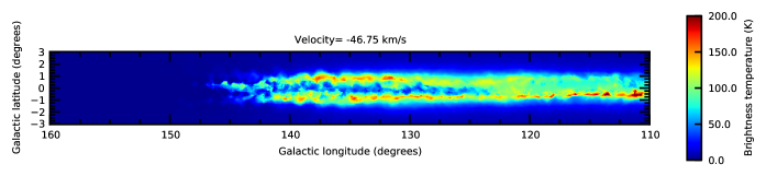
(a) NoFeedback

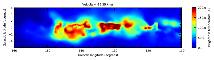
(b) Feedback5

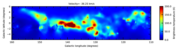
(c) Feedback10

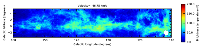
(d) CGPS

Figure 1: Brightness temperature of Hi emission, in Galactic latitude and longitude co-ordinates, from the Perseus arm in the CGPS and Perseus arm analogues in the synthetic data. The longitude coverage is the same in each case but the latitude coverage varies according to the extent of Hi emission (synthetic data) or survey coverage (CGPS). Fig. 1(a) is from a model galaxy without feedback, Fig. 1(b) is from a model galaxy with feedback and 5 per cent star formation efficiency, Fig. 1(c) is from a model galaxy with feedback and 10 per cent star formation efficiency, and Fig. 1(d) is from the Canadian Galactic Plane Survey.

The CGPS data show a broad region of emission which, in places, extends beyond $\pm 2$ degrees outside the mid-plane. In contrast the NoFeedback run has emission which is much more confined to the mid-plane, with bright ridges of emission at $\pm 1$ degree which are not seen in the CGPS data. Without feedback the gas in the model galaxy is overly confined to the mid-plane, resulting in large mid-plane optical depths. In the NoFeedback model the column density is highest within $\pm 1$ degree of the mid-plane but the accumulation of cold, dense material results in excessively high absorption and correspondingly low levels of Hi emission (in the optically thick limit the brightness temperature will saturate at the spin temperature). When feedback is included (Fig. 1(b) and 1(c)) the gas in the model galaxy is much less confined to the mid-plane and the bright ridges of emission, seen in Fig. 1(a) at about 1 degree above and below the mid-plane, are not present. The Hi emission now extends further out of the mid-plane, in better agreement with the CGPS observations.

Feedback results in significant holes in Hi emission, with Feedback10 in particular having much less contiguous emission than the CGPS observations. The CGPS observations have small scale filamentary structure, which is not seen in the synthetic observations, however, we do not expect to reproduce this structure at the current SPH resolution. The resolution of the SPH simulation is governed by the smoothing lengths of the particles. The density threshold for feedback to occur is at a number density of $1000\rm{cm}^{-3}$ which corresponds to a smoothing length of 5.6 pc (with a particle mass of $2500\rm{M}_{\odot}$). At a distance of 2.5 kpc (typical of material seen in Fig.1) this corresponds to an angular size of 0.13 degrees (or 7.8 arcmin). Structure on this scale is seen in the synthetic data (e.g. at $l=120$ in Fig 1(c)) but is spherical, rather than filamentary.

3.2 Vertical distribution of Hi emission

In order to allow a quantitative comparison of the vertical distribution of Hi emission, longitudinally averaged profiles of brightness temperature against latitude were extracted for the longitude range 126–144 degrees, in the same velocity channels shown in Fig. 1. Emission seen in this longitude and velocity range is from spiral arm material at a distance of approximately 2.5 kpc from the observer. At this distance material at a latitude of 1 degree is 44 pc out of the mid-plane.

The spiral arms in the simulations have a narrow velocity width, compared to the observed Perseus arm, and this results in emission from the simulated spiral arms being distributed over fewer velocity channels but with increased brightness temperatures (the structure of the arms in longitude-velocity space is discussed further in Section 3.3). Consequently the synthetic surveys have higher brightness temperatures than the CGPS data and the shape of the raw profiles cannot easily be compared. To facilitate a quantitative comparison the synthetic profiles were scaled by a constant scaling factor chosen to minimise the RMS difference from the CGPS data. The expression used to find the best value of the scaling factor $f$ was

$$\rm{RMS}=\sqrt{\frac{1}{N}\sum_{i=1}^{N}\left(C_{i}-fS_{j}\right)^{2}}$$ (1)

where $N$ is the number of points in the CGPS profile, $C_{i}$ is the brightness temperature in bin $i$ of the CGPS profile, and $S_{j}$ is the brightness temperature in bin $j$ of the synthetic profile, where bin $j$ and bin $i$ correspond in latitude. Every point in the brightness temperature profile was then scaled by the value of $f$ which minimised the expression in Eqn. 1. As the profiles are asymmetric the fit was repeated with the latitude axis inverted. The scaling factors and resultant RMS differences from the CGPS profile are shown in Table 1.

Table 1: Scaling factors applied to latitude profiles from synthetic data and the corresponding RMS differences from the CGPS profile.

Simulation	Scale factor	RMS	Reversed axis
		difference (K)	axis?
NoFeedback	0.82	28.6	No
Feedback5	0.535	8.86	No
Feedback10	0.762	8.20	No
NoFeedback	0.821	28.5	Yes
Feedback5	0.539	3.39	Yes
Feedback10	0.767	3.51	Yes

The scaled profiles and the unmodified CGPS profile are plotted in Fig. 2(a) and in Fig. 2(b) (with a reversed latitude axis in the second plot).

(a) Latitude axis not inverted

(b) Latitude axis inverted

Figure 2: Profiles of Hi brightness temperature with latitude. The solid line is from the CGPS, the dashed line is from the NoFeedback model, the dotted line is from Feedback5 and the dot-dashed line is from Feedback10. The normalisation of the synthetic profiles has been scaled to fit the CGPS data, so that the shape of the profiles can be readily compared. In Fig. 2(b) the latitude axis is inverted so that the synthetic profiles better match skewness of the CGPS profiles.

The fit for both the feedback runs is significantly better when the latitude axis is reversed, as the skewness of the profile better matches the skewness of the CGPS data. Both Feedback5 and Feedback10 fit the CGPS data well, provided the normalisation of the profile is scaled, and it is not possible to infer from these results whether 5% or 10% efficiency is a better fit to the data. Conversely the NoFeedback model does not fit the CGPS data well as the profile shows a large dip around the mid-plane giving a qualitatively different profile to that observed.

Although the star formation efficiency is different in Feedback5 and Feedback10, the rate of star formation is comparable at 250 Myr, as the process is largely self-regulating (as shown in fig. 11 of Dobbs et al. 2011a). Consequently the energy input from stellar feedback is similar for Feedback5 and Feedback10 (as the supernova rate is proportional to the star formation rate) and we expect the impact on the vertical distribution of Hi to be similar. Conversely a synthetic survey from a simulation with twice the surface density (run M10 from Dobbs et al. 2011a, not shown here) has a larger scale height than Feedback5 and Feedback10. This is consistent with the higher star formation rate (approximately four times higher) and an increased level of stellar feedback.

The amount of energy injected into the ISM in the simulations is directly proportional to the star formation rate. The star formation rate (SFR) in the Feedback5 and Feedback10 models is $\sim 0.7{\rm{M}}_{\odot}/{\rm{year}}$, which is consistent with the lower limit of the observationally determined Galactic star formation rate of Robitaille & Whitney (2010) but approximately a factor 2 less than the SFR of Murray & Rahman (2010). We note that SFRs determined from both observations and models are sensitive to assumptions about the slope and limits of the IMF (Calzetti et al., 2009). Additionally we can only insert feedback on a resolvable scale in the simulations, and cannot take into account all the sub-resolution processes which may dissipate or radiate energy. Hence we cannot definitively say how well energy injection in the models is similar to that in the Milky Way. However the effect of feedback has clearly been to make the models more realistic in this regard.

3.3 Longitude-velocity structure

Longitude-velocity plots in the Galactic mid-plane are shown in Fig. 3.

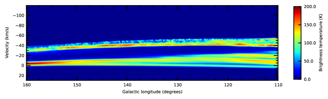
(a) NoFeedback

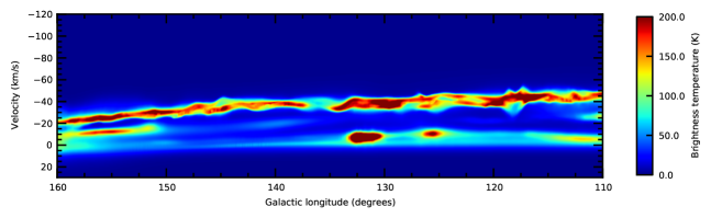
(b) Feedback5

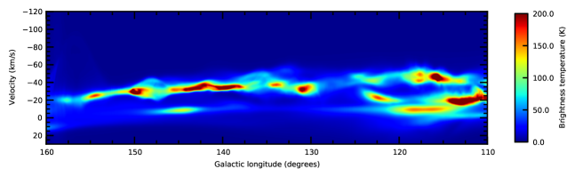
(c) Feedback10

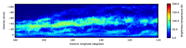
(d) CGPS

Figure 3: Brightness temperature of Hi emission, in Galactic longitude-velocity co-ordinates in the Galactic mid-plane. Fig. 3(a) is from a model galaxy without feedback, Fig. 3(b) is from a model galaxy with feedback and 5 per cent star formation efficiency, Fig. 3(c) is from a model galaxy with feedback and 10 per cent star formation efficiency, and Fig. 3(d) is from the Canadian Galactic Plane Survey.

These plots show local material around v=0 and Perseus arm material at more negative velocities (between $-20$ and $-60$ km/s). The inclusion of feedback results in much more structure in the spiral arms in longitude-velocity space. In Feedback5 the Perseus arm material is contiguous but structured, whereas in Feedback10 the Perseus arm material appears less contiguous. The local material is highly disrupted by feedback but as this material is close to the observer the angular size of the SPH smoothing length is large and the material is poorly resolved.

The CGPS data show material at more negative velocities than the simulations (beyond $-60$ km/s) but we would not expect to see material in this velocity range in the synthetic data because the model galaxies do not have a sufficiently large radial extent to represent this material. For gas in axisymmetric circular rotation the line of sight velocity (from equation 1 of Kalberla & Kerp (2009)) is

$$v\left(R,z\right)=\left[\frac{R_{\odot}}{R}\Theta\left(R,z\right)-\Theta_{\odot}\right]\sin l\cos b$$ (2)

where $v\left(R,z\right)$ is the line of sight velocity at point $\left(R,z\right)$, $\Theta\left(R,z\right)$ is the tangential velocity at $\left(R,z\right)$, $\Theta_{\odot}$ is the observer’s tangential velocity, $R_{\odot}$ is the distance of the observer from the Galactic centre, and $l$ and $b$ are Galactic latitude and longitude. In our synthetic surveys the observer is located at $R_{\odot}=7.1~{}\rm{kpc}$ within a model galaxy with an outer extent of 10 kpc, and at both these locations the tangential velocity is close to 220 km/s. Hence for material in the Galactic plane ($b=0$) the line of sight velocity at the outer edge of the model galaxy is

$$v\left(R,z\right)=-63.8\sin l~{}\rm{km/s}$$ (3)

At $l=110$ the maximum extent in velocity space is expected to be $-60~{}{\rm{km/s}}$ decreasing to $-22~{}{\rm{km/s}}$ at $l=160$. This is in agreement with the most extreme negative velocities seen in the synthetic data in Fig. 3.

3.4 Expanding shells

Several shells of material are seen in the synthetic observations (see Fig. 4 for an example from the Feedback5 model), similar to shells seen in Hi observations (Heiles, 1979, 1984; Hu, 1981; McClure-Griffiths et al., 2002; Ehlerová & Palouš, 2005). Such structures are expected as a consequence of energy feedback from massive stars and the feature in Fig. 4 is associated with a feedback event which occurred 1.2 Myr earlier. The feedback event comprised 20 supernovae, an atypically energetic event, which injected a total of $2\times 10^{52}$ erg of energy into the ISM.

In longitude-latitude space (Fig. 4(a)) an expanding shell appears as a variable radius ring with a maximum radius at the central velocity of the material. The radius of the shell decreases in velocity channels away from the central value and terminates with two “caps” of emission from the front and back of the bubble. By calculating the average surface brightness in concentric annuli about the centre of the shell, the structure can be plotted in velocity-radius space. A plot of this type, made using the kshell tool from the karma software package, is shown in Fig. 4(b). In velocity-radius space the structure is an arch shape which confirms that this structure is indeed expanding.

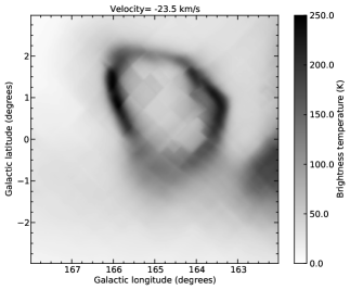
(a) Shell in longitude-latitude space

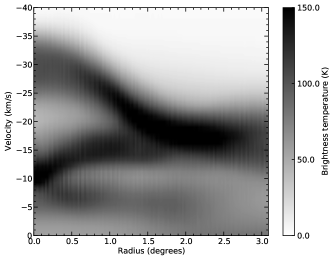
(b) Shell in velocity-radius space

Figure 4: An expanding shell of Hi emission from the Feedback5 model. The velocity-radius plot (right) shows the arch shape which is expected from an expanding shell. The angular offset is the radius of an annulus about the centre of the cell, where the centre is determined by eye.

Figure 4(b) shows that the shell has an expansion velocity of approximately 10 km/s and a maximum angular radius of approximately 2 degrees, which corresponds to 80 pc at 2.3 kpc (the distance from the observer’s position). The shell radius and expansion velocity are smaller than typical values from the samples of Heiles (1979) and Heiles (1984), however Heiles (1984) notes a bias towards selecting larger shells and our shell is more typical of the shells found by Hu (1981). The size of our shell is also consistent with the smaller shells in the sample of McClure-Griffiths et al. (2002), observed in the Southern Galactic Plane Survey.

4 Hi self-absorption

When generating synthetic observations the calculation of Hi intensity can be split into separate emitting and absorbing components. This allows us to produce a data cube containing only the absorption component, in order to identify where HISA is present. Furthermore, each cell of the AMR grid is identified as either a net source of emission or a net source of absorption by calculating the change in intensity due to the grid cell, normalised by the column density of the cell. The SPH particles are then associated with the change in emission from the AMR cell in which they reside, thus we are able to determine which SPH particles are responsible for HISA. Compared to observers we are in the privileged position of being able to unambiguously identify absorbing components in the data cube and furthermore we can identify absorption with specific SPH particles. In Section 4.1 we use the absorption-only data cubes to examine the distribution of HISA on the plane of the sky, then in Section 4.2 we use the identification of absorbing SPH particles to investigate the properties of the material which causes HISA.

4.1 HISA distribution

The velocity integrated absorption component is plotted in Fig. 5 for the NoFeedback, Feedback5 and Feedback10 models. Equivalent plots from the CGPS data are shown in figure 1 of Gibson et al. (2005).

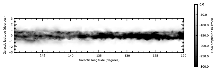
(a) NoFeedback

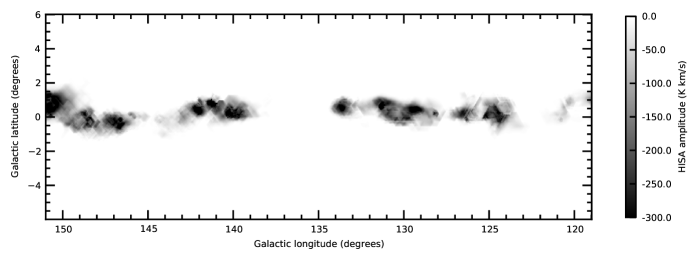
(b) Feedback5

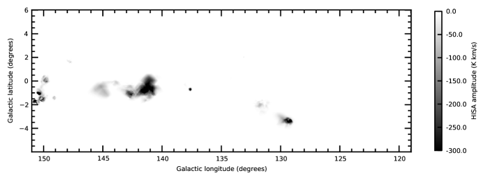
(c) Feedback10

Figure 5: Hi self-absorption amplitude, calculated from the synthetic observations, where the absorption is integrated over all velocity channels. Fig. 5(a) is from a model galaxy without feedback, Fig. 5(b) is from a model galaxy with feedback and 5 per cent star formation efficiency, Fig. 5(c) is from a model galaxy with feedback and 10 per cent star formation efficiency

In the NoFeedback model (Fig. 5(a)) there is a broad band of strong HISA, due to an over concentration of Hi in the mid-plane. HISA in the NoFeedback case is confined to $\pm 1$ degree from the mid-plane, whereas observed HISA has a greater vertical extent. The HISA morphology in the Feedback5 model is more realistic, with extended, low intensity HISA surrounding knots of stronger absorption. Both the morphology and vertical extent of the Feedback5 model are more similar to the CGPS observations of Gibson et al. (2005). Although the Feedback5 HISA has less substructure in the strong HISA complexes this is to be expected, given the small spatial scale of the observed structures relative to the model resolution. In the Feedback10 model the HISA has a much reduced diffuse component, compared to the other models. Gibson et al. (2005) find nearly ubiquitous weak HISA and in this regard the Feedback10 model does not match the observations. Models with higher star formation efficiencies have less material in the cold phase, as shown in fig. 4 of Dobbs et al. (2011a), so Feedback10 is expected to have less HISA than Feedback5 as there is less cold atomic hydrogen. We conclude that the Feedback5 model has a more realistic HISA morphology than either of the other models, albeit with limited spatial resolution.

4.2 Properties of material responsible for HISA

Figure 6 shows a histogram of number densities (Fig. 6(a)) and temperatures (Fig. 6(b)) for absorbing particles from Feedback5, located in the region used to generate the synthetic survey. The solid line is for all particles in a cell with net absorption (6% of particles in region), the dashed line is for particles associated with absorption stronger than $1\times 10^{-23}$ erg/s/sr (2% of particles in region) and the dotted line is for particles associated with absorption stronger than $2\times 10^{-23}$ erg/s/sr (1% of particles in region).

(a) Feedback5 number density

(b) Feedback5 temperature

(c) Feedback10 number density

(d) Feedback10 temperature

Figure 6: Number density and temperature distributions of SPH particles associated with Hi self-absorption (HISA). For the Feedback5 model three different absorption thresholds are used to define HISA particles: $dI<0$ (solid line), $dI<-1\times 10^{-23}$ erg/s/sr (dashed line), and $dI<2\times 10^{-23}$ erg/s/sr (dotted line). For the Feedback10 model there are fewer HISA particles and only one line is plotted (particles with $dI<0$).

There is no evidence for particles associated with stronger HISA to be higher density or at a lower temperature, indeed the temperature range is 10-100K (typical of the cold neutral interstellar medium) for almost all the absorbing particles. For these histograms the mean Hi number density is 130–190 $\rm{cm}^{-3}$ and the mean temperature is 32–36 K.

The density and temperature distributions for absorbing particles from Feedback10 are shown in Fig. 6(c) and Fig. 6(d) respectively. Particles associated with net absorption are plotted as a solid line but no other thresholds are used, as the number of absorbing particles is much smaller than for Feedback5 (1% of particles are absorbing in Feedback10). For Feedback10 the mean Hi number density is 490 $\rm{cm}^{-3}$ and the mean temperature is 27K. The range of temperatures and densities seen in Feedback10 are similar to those seen in Feedback5, although the HISA in Feedback10 is from slightly colder and denser material. The star formation efficiency has only a modest effect on the properties of material seen in HISA, even though the morphology of the HISA is significantly different.

In their study of HISA clouds in Perseus, Klaassen et al. (2005) found number densities between $100~{}\rm{cm}^{-3}$ and $1200~{}\rm{cm}^{-3}$, and spin temperatures in the range 12K–24K, in an extended HISA cloud which they term the “complex”. In a smaller, isolated HISA feature, which they term the “globule”, the spin temperatures were in the range 8K–22K (no density determination was made for the globule.) The globule is a compact structure (unresolved in the 1 arcmin main beam of the CGPS) and is much smaller than the resolution limit of our synthetic observations (see section 3.1). The complex region is much larger and hence is more like the HISA clouds seen in our synthetic data. The density of HISA producing material in Feedback5 and Feedback10 is consistent with the density of the complex region found by Klaassen et al. (2005). Although the mean temperature of our HISA producing material is slightly higher than the temperatures found by Klaassen et al. (2005) we note that there is sufficient spread in our temperature values to encompass their observationally determined temperatures (see Fig. 6(b) and Fig. 6(d)). Material can drop out of the gas phase and form supernovae above a density of $1000~{}\rm{cm}^{-3}$, so the densest and coldest regions of HISA producing gas (seen in the observations) are at the limit of the SPH simulations’ representation.

The next point to be addressed is whether particles which contribute to HISA are in a different phase to other particles at similar temperatures, and whether HISA producing material is in pressure balance with other material. In Fig. 7 we plot pressure against number density for HISA particles (Fig. 7(a)) and for all other particles with a temperature below 150K (Fig. 7(b)). There are approximately five times as many particles in Fig. 7(b) as in Fig. 7(a), indicating that there is a significant amount of cold, dense Hi which is not observed in HISA.

(a) HISA particles

(b) Other particles

Figure 7: Plots of pressure against number density for particles producing Hi self-absorption (Fig. 7(a)) and all other particles with temperatures below 150K (Fig. 7(b)), showing that HISA particles are not over-pressured compared to other cold particles.

For particles with a number density above $10^{2}\rm{cm}^{-3}$ there is no apparent difference between the two populations. At lower densities the distributions are also similar but there is more spread (towards higher pressures) in the non-HISA particles. The thermal pressure of HISA material does not appear to be significantly different to other material, although we note that the effect of velocity dispersion has not been included here, which would provide support against gravity in addition to thermal pressure.

Although the material responsible for HISA is identifiable as the cold neutral medium, which is expected to go on to form stars, we can be more specific about the fate of the SPH particles responsible for HISA. Particles which are in giant molecular clouds (GMCs) are identified, using the clump finding algorithm of Dobbs et al. (2008), and correlated with whether the material is also observed in HISA. In the Feedback5 model 4.0% of the HISA particles are in GMCs, compared to 2.2% of material in GMCs for the galaxy as a whole, and 70% of HISA material is involved in a feedback event (i.e. involved in star formation) within the next 20 Myr. The fraction of HISA material in clouds, and the fraction which forms stars, is not found to vary with HISA strength. For Feedback10 we find that 2.5% of HISA material is in GMCs, compared to 0.9% in the galaxy as a whole, and 57% of HISA material goes on to be involved in star formation.

5 Conclusions and Discussion

The inclusion of feedback in the galaxy models has a significant effect on the derived synthetic Hi Galactic plane surveys. In the model without feedback (NoFeeback) gas is overly confined to the mid-plane, which results in excessive absorption. Consequently there are bands of bright emission above and below the mid-plane (which are not seen in observations) and the vertical extent of the Hi emission is too small. The two models which include feedback (Feedback5 and Feedback10) both have a larger vertical extent of Hi emission and their profiles of Hi emission with latitude match the CGPS observations well (provided the normalisation is allowed to vary). Based on the vertical distribution of Hi emission alone it is not possible to determine whether Feedback5 or Feedback10 is more realistic.

When feedback is included more structure is seen in Hi emission, including bubbles of material associated with supernova events, however the model does not yet have sufficient spatial resolution to capture the very fine scale structure seen in the CGPS data. With increases in available computing power it will be feasible to run the SPH simulations using more particles, giving a higher spatial resolution. This should result in more realistic small scale structure in the synthetic observations. However if the filamentary structure is due to the presence of magnetic fields then these too will need to be included before a good match with the observed Hi morphology on a small scale can be expected.

One further respect in which the synthetic data are more realistic is the properties of HISA. The NoFeedback model has a broad band of strong HISA, unlike HISA seen in observations. When feedback is included with 5 per cent star formation efficiency the HISA structure is much more like that in the observations of Gibson et al. (2005). However if the star formation efficiency is increased to 10 per cent there is insufficient HISA, in particular there is no ubiquitous weak HISA as found by Gibson et al. (2005). Based on the HISA morphology we conclude that a 5 per cent star formation efficiency is more realistic than a 10 per cent star formation efficiency.

With the simulations with feedback the HISA distribution is more realistic and it is meaningful to examine the properties of material which is seen in HISA. The temperature and density properties are confined to a well defined range (typical of cold Hi) which is independent of how strongly the material is absorbing, and only weakly dependent on the star formation efficiency. Although the correspondence between HISA and molecular clouds is not one-to-one it is clear that HISA preferentially selects material in GMCs. However the nature of clouds is dynamic and a given cloud will not be composed of the same material as it evolves. Consequently material which is seen in HISA at any given time may become part of a GMC later, and HISA material currently in a GMC can leave the cloud at a later time. Understanding the complex relationships between HISA, GMC material and star formation could be facilitated with a time series of synthetic observations, which would track particles, determine when they are observable as HISA, and correlate this with the molecular gas fraction.

References

- Acreman et al. (2010) Acreman D. M., Douglas K. A., Dobbs C. L., Brunt C. M., 2010, MNRAS, 406, 1460
- Allen et al. (2004) Allen R. J., Heaton H. I., Kaufman M. J., 2004, ApJ, 608, 314
- Bagetakos et al. (2011) Bagetakos I., Brinks E., Walter F., de Blok W. J. G., Usero A., Leroy A. K., Rich J. W., Kennicutt Jr. R. C., 2011, AJ, 141, 23
- Bergin et al. (2004) Bergin E. A., Hartmann L. W., Raymond J. C., Ballesteros-Paredes J., 2004, ApJ, 612, 921
- Calzetti et al. (2009) Calzetti D., Sheth K., Churchwell E., Jackson J., 2009, in The Evolving ISM in the Milky Way and Nearby Galaxies Star Formation Rate Determinations in the Milky Way and Nearby Galaxies
- Chevalier (1974) Chevalier R. A., 1974, ApJ, 188, 501
- Cowie (1981) Cowie L. L., 1981, ApJ, 245, 66
- Dobbs (2008) Dobbs C. L., 2008, MNRAS, 391, 844
- Dobbs et al. (2011a) Dobbs C. L., Burkert A., Pringle J. E., 2011a, MNRAS, 417, 1318
- Dobbs et al. (2011b) Dobbs C. L., Burkert A., Pringle J. E., 2011b, MNRAS, 413, 2935
- Dobbs et al. (2008) Dobbs C. L., Glover S. C. O., Clark P. C., Klessen R. S., 2008, MNRAS, 389, 1097
- Douglas et al. (2010) Douglas K. A., Acreman D. M., Dobbs C. L., Brunt C. M., 2010, MNRAS, 407, 405
- Douglas & Taylor (2007) Douglas K. A., Taylor A. R., 2007, ApJ, 659, 426
- Ehlerová & Palouš (2005) Ehlerová S., Palouš J., 2005, A&A, 437, 101
- Fukui et al. (2009) Fukui Y., Kawamura A., Wong T., Murai M., Iritani H., Mizuno N., Mizuno Y., Onishi T., Hughes A., Ott J., Muller E., Staveley-Smith L., Kim S., 2009, ApJ, 705, 144
- Gibson et al. (2005) Gibson S. J., Taylor A. R., Higgs L. A., Brunt C. M., Dewdney P. E., 2005, ApJ, 626, 195
- Goldsmith & Li (2005) Goldsmith P. F., Li D., 2005, ApJ, 622, 938
- Harries (2000) Harries T. J., 2000, MNRAS, 315, 722
- Heiles (1979) Heiles C., 1979, ApJ, 229, 533
- Heiles (1984) Heiles C., 1984, ApJS, 55, 585
- Hennebelle et al. (2007) Hennebelle P., Audit E., Miville-Deschênes M.-A., 2007, A&A, 465, 445
- Hu (1981) Hu E. M., 1981, ApJ, 248, 119
- Kalberla & Kerp (2009) Kalberla P. M. W., Kerp J., 2009, ARA&A, 47, 27
- Kaufman et al. (1999) Kaufman M. J., Wolfire M. G., Hollenbach D. J., Luhman M. L., 1999, ApJ, 527, 795
- Kavars et al. (2005) Kavars D. W., Dickey J. M., McClure-Griffiths N. M., Gaensler B. M., Green A. J., 2005, ApJ, 626, 887
- Kim et al. (2008) Kim C.-G., Kim W.-T., Ostriker E. C., 2008, ApJ, 681, 1148
- Klaassen et al. (2005) Klaassen P. D., Plume R., Gibson S. J., Taylor A. R., Brunt C. M., 2005, ApJ, 631, 1001
- Li & Goldsmith (2003) Li D., Goldsmith P. F., 2003, ApJ, 585, 823
- McClure-Griffiths et al. (2002) McClure-Griffiths N. M., Dickey J. M., Gaensler B. M., Green A. J., 2002, ApJ, 578, 176
- McKee & Ostriker (1977) McKee C. F., Ostriker J. P., 1977, ApJ, 218, 148
- Murray & Rahman (2010) Murray N., Rahman M., 2010, ApJ, 709, 424
- Parkin (2011) Parkin E. R., 2011, MNRAS, 410, L28
- Price & Monaghan (2007) Price D. J., Monaghan J. J., 2007, MNRAS, 374, 1347
- Roberts (1972) Roberts Jr. W. W., 1972, ApJ, 173, 259
- Robitaille & Whitney (2010) Robitaille T. P., Whitney B. A., 2010, ApJL, 710, L11
- Rundle et al. (2010) Rundle D., Harries T. J., Acreman D. M., Bate M. R., 2010, MNRAS, 407, 986
- Shetty et al. (2011) Shetty R., Glover S. C., Dullemond C. P., Klessen R. S., 2011, MNRAS, 412, 1686
- Shetty & Ostriker (2008) Shetty R., Ostriker E. C., 2008, ApJ, 684, 978
- Tasker & Tan (2011) Tasker E. J., Tan J. C., 2011, in J. Alves, B. G. Elmegreen, J. M. Girart, & V. Trimble ed., IAU Symposium Vol. 270 of IAU Symposium, Star Formation and the Properties of Giant Molecular Clouds in Global Simulations. pp 377–380
- Taylor et al. (2003) Taylor A. R., Gibson S. J., Peracaula M., Martin P. G., Landecker T. L., Brunt C. M., Dewdney P. E., Dougherty S. M., Gray A. D., Higgs L. A., Kerton C. R., Knee L. B. G., Kothes R., Purton C. R., Uyaniker B., Wallace B. J., Willis A. G., Durand D., 2003, AJ, 125, 3145
- Wada (2008) Wada K., 2008, ApJ, 675, 188
- Wolfire et al. (2003) Wolfire M. G., McKee C. F., Hollenbach D., Tielens A. G. G. M., 2003, ApJ, 587, 278
- Woltjer (1972) Woltjer L., 1972, ARA&A, 10, 129