Radioscience simulations in General Relativity and in alternative theories of gravity

Abstract

This paper deals with tests of General Relativity in the Solar System using tracking observables from planetary spacecraft. We present a new software that simulates the Range and Doppler signals resulting from a given space-time metric. This flexible approach allows one to perform simulations in General Relativity as well as in alternative metric theories of gravity. The outputs of this software provide templates of anomalous residuals that should show up in real data if the underlying theory of gravity is not General Relativity. Those templates can be used to give a rough estimation of constraints on additional parameters entering alternative theory of gravity and also signatures that can be searched for in data from past or future space missions aiming at testing gravitational laws in the Solar System. As an application of the potentiality of this software, we present some simulations performed for Cassini-like mission in Post-Einsteinian Gravity and in the context of MOND External Field Effect. We derive signatures arising from these alternative theories of gravity and estimate expected amplitudes of the anomalous residuals.

1 Introduction

Testing General Relativity (GR) is a long standing and worthy effort in the scientific community. From a theoretical point of view, the different attempts to quantize gravity or to unify it with the other fundamental interactions always predict deviations from GR. From an observational point of view, cosmological data cannot be explained by the combination of GR and the standard model of particles. In the most accepted cosmological model, the so-called $\Lambda$CDM model, these observations are explained by the presence of two puzzling ingredients: Dark Matter and Dark Energy, representing respectively about 22 % and 74 % of the Universe. Until today, these two dark components have not been observed directly. Therefore these cosmological observations can be a hint that General Relativity may not be the correct theory of gravitation at large scales.

Up to now, GR has passed all the critical tests in the different situations where it has been tested. In the Solar System, the tests of gravitation mainly rely on the parameterized Post-Newtonian (PPN) formalism [1, 2] or on a search for a deviation from the Newtonian potential of the Yukawa type (the so-called fifth force search). In the PPN framework the space-time metric is parameterized by 10 constant coefficients (the most important ones being $\gamma$ that characterizes the spatial curvature and $\beta$ that characterizes the non-linearity of the theory). The current constraints on these coefficients are very stringent as described in Will [2]. For example, the $\gamma$ parameter is constrained at the level of $10^{-5}$ by the measurement of the Shapiro delay using the Cassini spacecraft [3] while the $\beta$ parameter is now constrained at the level of $10^{-5}$ with planetary ephemeris [4], Lunar Laser Ranging [5] and with the tracking of Mars orbiters [6]. In the fifth force framework (described in [7, 8, 9, 10]), the gravitation theory is very well tested at almost all scales as can be seen from figure 31 of [6]. Nevertheless, there are still two main open windows where potential deviations can be expected: at small scales in the laboratory and at outer solar-system scales. In this context, let us mention the existence of an anomalous acceleration recorded on Pioneer 10/11 probes during their flight to the outer solar system [11, 12, 13] (for a review, see [14] and references therein). If recent publications [15, 16] seem to indicate that part of the secular anomaly could be accounted by thermal effects, other features such as modulations call for another explanation.

Given the existing stringent constraints, there are strong motivations to move forward in the search for deviations from GR in the Solar System. First of all, to push for higher precision experiments remains a valuable challenge. This is motivated by some scenarios of alternative theories of gravity producing deviations smaller than the current constraints. Let us mention in this context certain types of tensor-scalar theories where the cosmological evolution exhibits an attractor mechanism that attracts the theory towards GR [17, 18] or chameleon theories [19, 20, 21] where the deviations from GR are hidden in the region of the Universe where the matter density is high (as inside the solar system). Both of these alternative theories of gravity produce a deviation of the $\gamma$ PPN parameter smaller than the current constraint. There exist also open windows in existing frameworks where deviations can be searched at very small distances and at very large distances (in the outer Solar System). Finally, it is useful to analyze experimental results in new extended frameworks. Indeed, even if observations lie very close to GR when analyzed within the PPN or fifth force framework, this does not mean that this has to be true in any other framework. The existing frameworks indeed cover a limited set of alternative theories of gravity. A formalism based on a non-local Einstein field equation more adapted for quantization has thus been developed in a series of recent papers [22, 23, 24, 25, 26]. In this extension of GR, the modification of the space-time metric in the Solar System is phenomenologically described by two functions depending on position. As is also the case in $f(R)$ theories exhibiting a chameleon mechanism [27, 28, 29], the PPN parameters are then promoted to functions depending on position. A last example is given by the Standard Model Extension (SME) framework where Lorentz symmetry is broken. In the gravitational sector, SME is characterized by a metric which goes beyond the existing framework [30, 31].

In this paper, we focus on Solar System tests of gravity. In this context, the gravitational observations rely either on astrometric observations (right ascension and declination), with the advantage of very long measurement time, or on spacecraft tracking (radioscience measurement : Range, Doppler, VLBI), with the advantage of very high precision but limited time span. Here, we only consider radioscience measurements based on Range and Doppler (future work will consider angular measurements).

Our present work is part of a long term project aiming at allowing, systematic and versatile scanning of data from solar system observations (e.g. spacecraft Range, Doppler, VLBI, angular measurements, astrometry, …) looking for possible violations of the known laws of gravitation (General Relativity). By this we mean that the same basic procedure can be systematically applied to all different types of data, or their combination; and by versatile we mean that the procedure is easily adapted to any alternative theory that is tested for, provided the space-time metric of that theory is available.

The basic procedure, when completed, will consist of the following steps:

1. Simulate the observables of a given physical situation (eg. an arc of spacecraft tracking from Earth) in the alternative theory. In this step, a simplified version of the physical situation can be considered: only the elements that can give rise to leading order deviations due to the alternative theory need to be simulated.

2. Analyze the resulting observables using the usual procedure in GR: fit a GR model on the data by adjusting the initial conditions of the different bodies and the parameters entering the modeling [32]. The residuals of that analysis provide the incompressible signal that should be present in the residuals of the real data of the considered physical situation if the gravitation theory in the solar system is not GR but the one used in the first step. These residuals are called incompressible in the sense that this part of the signal can not be absorbed anymore by a fit of real or simulated (in an alternative theory of gravity) data using a GR model.

3. Analyze the real data using the usual procedure in GR (including all known systematic effects eg solar radiation, thermal effects, all gravitational perturbations, etc…). This analysis provides residuals of a fit of real data using a GR model.

4. Systematically search the residuals of step (iii) (obtained from real data) using the ”template” obtained in step (ii). This can be done by optimal filtering, matched filtering or any other statistical method best adapted to the data and template. If the template is found with a S/N $>$ 1 the alternative theory considered is better supported by the data than GR. Depending on the S/N one can then consider the result significant or not, and start searching for systematic effects that might explain it (helped by the detailed signature of the template) and/or try other physical situations (other spacecraft, other types of observation, etc…) to confirm the result.

In this paper we present a first version of the step (i) and a simplified version of the step (ii). The simulation software is built in the spirit that everything is computed from the space-time metric (computation of trajectories, clock behavior, light propagation). This software allows simulation of spacecraft Range and Doppler observations in any alternative theory for which a metric is available. Note that in the first step only the leading order effects need to be considered, as we expect the modifications of second order effects (eg. solar radiation, thermal effects, gravitational perturbations, …) by the alternative theory to be negligible with respect to the leading order. However, step (ii) needs to include all effects that could absorb some of the anomalous residuals by fitted parameters of the perturbations. Some care is required concerning the coherence between steps (i) and (ii), to ensure that no ”false” signals are generated by perturbations included in step (ii) but not in (i). As an example, including perturbations by an additional planet in only step (ii) (but not (i)) will significantly modify the residuals (obtained from simulated data), but including it in both or neither gives rise to essentially the same residuals (cf. section 5.1 for an explicit example using Jupiter). In the simplified version presented here the second step uses only the main features of a full analysis in GR (neglecting eg. solar radiation pressure, thermal effects, planetary gravitational fields, etc…).

Nonetheless this allows us to derive the general form of the expected templates for a given physical situation in alternative theory, although some of the features of those templates will be modified (absorbed by additional parameters) when carrying out a complete fit in the second step. Furthermore, we can compare the maximum amplitude of those templates to the typical rms noise of residuals from real spacecraft tracking, thereby giving a rough order of magnitude of the expected constraints when a full analysis of the type above is applied to existing data. On one hand the constraints in a full analysis will be more stringent than these rough orders of magnitude because optimum filtering will perform better than a simple comparison of the residual rms to the template amplitude. On the other hand they will be less stringent because some of the features of the signature will be absorbed by additional parameters that are not present in our simplified version of step (ii). Finally, for future missions our procedure will allow optimizing the mission characteristics (trajectories, periods of observation, maneuvers, etc…) for optimum tests of alternative theories by maximizing the signatures in the templates.

The procedure presented above is significantly easier to apply (once the software for steps (i) and (ii) exists) and more versatile, than to write a complete data analysis software in an alternative theory. The main reason for that is that in steps (i) and (ii) a simplified situation is sufficient to obtain the correct template. It is not necessary to include all perturbing effects (solar radiation pressure, all planets and asteroids, thermal radiation, etc…) at this stage. The full analysis including all effects is carried out in step (iii) using existing software in GR. Furthermore residuals from step (iii) are in general more readily available and easier to handle than raw data from the observations.

2 Outline

The method used to simulate Range and Doppler observations directly from the space-time metric is presented in detail in section 3. The definitions of the observables (Range and Doppler) are given and the methodology used to simulate such observables is presented step by step: the derivation and the integration of the equations of motion, the behavior of the clocks and the propagation of light in curved space-time. With this software, it is possible to simulate radioscience signals in alternative theories of gravity.

In section 4, we explain the method used to analyze signals obtained. In particular, the least-square fit of the initial conditions is briefly described and an estimation of the numerical accuracy of the whole process (simulation and fit procedure) is presented.

Section 5 presents the original results of this paper. Explicit simulations are performed for Range and two-way Doppler between Earth and the Cassini spacecraft during its cruise between Jupiter and Saturn (from May 2001). In this paper, we focus on two classes of alternative theories: the Post-Einsteinian Gravity and MOND External Field Effect [33, 34]. We now briefly introduce these two alternative theories of gravity in the remainder of this section.

2.1 Post-Einsteinian Gravity (PEG):

The first alternative metric theory considered is Post-Einsteinian Gravity (PEG in the following) [22, 23, 24, 25, 26]. In this theory, the geometric features of general relativity such as the identification of gravitational fields with the metric and the equivalence principle are preserved but the form of the Einstein equations is modified. This theory relies on the existence of a quantized gravitation and is non-local because of radiative corrections. The relation between the curvature and the stress energy tensor (which is local in GR) is generalized such that it takes the form of a non local response relation [24]. The Einstein equations for a static spherical body are characterized by two running constants which take the place of the Newton gravitation constant [22]. Within the perturbative approximation valid in the Solar System, the metric is characterized by two potentials $\phi_{N}$ and $\phi_{P}$. In isotropic gauge, the metric tensor for a spherical source can be written as

$$g_{00} = 1+2\phi_{N}=1+2\phi(r)+2\phi(r)^{2}+2\delta\phi_{N}(r)$$ (1a)

$$g_{ij} = \delta_{ij}\left(-1+2\phi_{N}-2\phi_{P}\right)=\delta_{ij}\left(-1+2\phi(r)+2\delta\phi_{N}-2\delta\phi_{P}\right)$$ (1b)

where $\phi(r)=-\frac{GM}{rc^{2}}$ is the Newtonian potential with $G$ the Newton constant, $M$ the mass of the central body, $c$ the speed of light, $r$ the radial coordinate while $\delta\phi_{N}(r)$ and $\delta\phi_{P}(r)$ are two functions of the position characterizing the deviation from GR. The Post-Newtonian formalism (PPN) is recovered for particular potentials

$$\delta\phi_{N}(r) = (\beta-1)\phi(r)^{2}$$

$$\delta\phi_{P}(r) = -(\gamma-1)\phi(r)+(\beta-1)\phi(r)^{2}\cdot$$

In order to derive constraints on these functions, we will consider a series expansion of the two potentials [35]

$$\delta\phi_{N}(r) = \alpha_{1}r+\alpha_{2}r^{2}+\frac{GM}{c^{2}\Lambda}\log\frac{r}{\Lambda}$$ (1ba)

$$\delta\phi_{P}(r) = \chi_{1}r+\chi_{2}r^{2}-\delta\gamma\frac{GM}{c^{2}r}$$ (1bb)

where $\alpha_{1,2}$, $\chi_{1,2}$ and $\Lambda$ are PEG parameters and $\delta\gamma=\gamma-1$ is the traditional PPN parameter. These coefficients are related to coefficients appearing in the generalized Einstein field equations which have the form of a non-local relation between the curvature and the stress energy tensor.

The expansion (1ba-1bb) can also be seen from the perspective of the Ricci tensor. In vacuum, the GR Ricci tensor vanishes, the spatial part of the PPN Ricci tensor decreases as $1/r^{3}$. The extension to the above metric gives a Ricci tensor with a spatial part decreasing as $1/r^{2}$ (for the logarithmic term), as $1/r$ (for the linear term) or remaining constant (for the quadratic term). It can be noted that a linear and a quadratic term in the space-time metric naturally appear in conformal theory of gravity [36] and in this context can also be invoked to explain certain galactic observations requiring dark matter. The logarithmic term produces a $1/r$ modification of the Newtonian gravitational force which can be used to explain certain observations requiring dark matter [37, 38, 39].

2.2 MOND External Field Effect (EFE):

The second alternative theory of gravity considered is the External Field Effect (EFE in the following) produced by MOND theory. The MOND theory [40] consists in a modification of the gravity law at low acceleration. Naively one would therefore expect no significant modification in the solar system, where the gravitational acceleration is large. Nevertheless Milgrom [41] and later Blanchet and Novak [33] have shown that MOND theory predicts a violation of the strong equivalence principle which implies that the dynamics of a system is influenced by an external gravitational field. This EFE implies the presence of an anomalous quadrupolar correction in the Newtonian potential  [33, 41]

$$\phi=-\frac{GM}{r}-\frac{Q_{2}}{2}x^{i}x^{j}\left(e_{i}e_{j}-\frac{1}{3}\delta_{ij}\right)$$ (1bc)

where $e_{i}$ is a unitary vector pointing towards the galactic center. The value of the quadrupole $Q_{2}$ can be computed from the theoretical model of MOND and depends on the MOND interpolating function. Let us mention that in Blanchet and Novak [33], the value of $Q_{2}$ has been determined numerically and is framed by two limits,

$$2.1\times 10^{-27}\ s^{-2}\leq Q_{2}\leq 4.1\times 10^{-26}\ s^{-2}$$ (1bd)

depending on the MOND function used. The modification of the metric deriving from this modification of the Newtonian potential can be expressed using the metric parametrization (1a-1b) with

$$\delta\phi_{N} = -\frac{Q_{2}}{2c^{2}}x^{i}x^{j}\left(e_{i}e_{j}-\frac{1}{3}\delta_{ij}\right)$$ (1bea)

$$\delta\phi_{P} = 0.$$ (1beb)

Blanchet and Novak [33, 34] have also shown that this quadrupolar term implies the existence of a secular precession of planetary perihelia. New improved INPOP results [4] on planetary perihelion precession put an even more stringent constraint on the quadrupole [34].

3 Numerical simulations of observables from the space-time metric

In this section, we present the numerical methods used to simulate Range and Doppler signals directly from the space-time metric. First of all covariant definitions of the observables are given. After, we explain in detail the different steps needed to simulate signals from the metric. This includes the derivation and integration of the equations of motion, the derivation and integration of the equation of proper-time and the computation of the propagation of light in curved space-time and the determination of the observables.

3.1 Tracking observables

Observables, that is to say measured quantities, are by definition gauge invariant : they do not depend on the choice of a coordinate system. The simulations, for example the integration of the equations of motion, are necessarily done in a particular coordinate system (different equations of motion representing the same situation in different coordinates system can be found in [42, 43]). A reduction of coordinates, that is to say a transformation of coordinate-dependent quantities to measurable quantities (observables) is done in the software and presented below.

The situation corresponding to traditional radioscience measurements is the following : an electromagnetic signal is sent by an emitter (denoted by subscript $e$), eventually re-transmitted by a transponder (denoted by $t$) and received by an observer (denoted by $r$) which is often the same as the emitter. The emitted signal is characterized by its proper frequency $\nu_{e}$ and by the emission proper time $\tau_{e}$ (time when the signal is sent as given by an ideal clock moving with the emitter). Similarly the received signal is characterized by its proper frequency $\nu_{r}$ and by the reception proper time $\tau_{r}$.

The Range signal (evaluated at reception) is related to the signal propagation time between the emitter and the receiver:

$$R(\tau_{r})=c(\tau_{r}-\tau_{e})\cdot$$ (1bef)

The Doppler signal is related to the frequency shift between the emitter and the receiver:

$$D(\tau_{r})=\frac{\nu_{r}}{\nu_{e}}\cdot$$ (1beg)

These definitions are based on proper quantities that are measurable.

3.2 Equations of motion

The equations of motion are directly derived from the metric using the geodesic equations [44, 43], integrated with respect to coordinate time $t$:

$$\frac{1}{c^{2}}\frac{d^{2}x^{i}}{dt^{2}}=-\Gamma^{i}_{00}-2\Gamma^{i}_{0j}\beta^{j}-\Gamma^{i}_{jk}\beta^{j}\beta^{k}+\Gamma^{0}_{00}\beta^{i}+2\Gamma^{0}_{0j}\beta^{i}\beta^{j}+\Gamma^{0}_{jk}\beta^{i}\beta^{j}\beta^{k}$$ (1beh)

where $x^{i}$ are the spatial coordinates of the test particle, $\beta^{i}=v^{i}/c$ is the reduced coordinate velocity, $\Gamma^{\alpha}_{\beta\gamma}$ are the Christoffel symbols of the considered metric (Greek indices run from $0$ to $3$ while Latin indices from $1$ to $3$) and $t$ is coordinate time. The Christoffel symbols are computed using the metric and its first derivatives

$$\Gamma^{\alpha}_{\beta\gamma}=\frac{1}{2}g^{\alpha\delta}\left(g_{\delta\gamma,\beta}+g_{\beta\delta,\gamma}-g_{\beta\gamma,\delta}\right)$$ (1bei)

with $g^{\alpha\delta}$ the inverse of the metric $g_{\alpha\delta}$, $g^{\alpha\delta}g_{\delta\beta}=\delta^{\alpha}_{\beta}$. In our approach, we choose to implement analytically the derivative of the metric so that the Christoffel symbols and the right hand side of Equation (1beh) can be computed exactly. Let us mention the other possibility consisting in implementing a numerical derivative of the space-time metric [45]. Nevertheless, the numerical accuracy of the derivative can be problematic and is time-consuming.

The software is independent of any ephemerides. This choice is justified since external ephemerides (such as INPOP [46, 4], DE [47] or EPM [48]) are computed in General Relativity or within PPN formalism [49, 50, 51] and the goal of our approach is to go beyond the latter. In order to be fully consistent, we produce the ephemerides needed by integrating the equations of motion of all bodies considered in the problem, here the spacecraft, the Sun and the Earth (observer), in the theory considered.

3.3 Clock behavior

In the process of reduction to relativistic observables, the proper time equation is integrated for each body considered, and in particular for the clocks used in the Doppler/Range measurements. This equation is

$$\frac{d\tau}{dt}=\sqrt{g_{00}+2g_{0i}\beta^{i}+g_{ij}\beta^{i}\beta^{j}}$$ (1bej)

where $g_{\mu\nu}$ is the space-time metric and $\tau$ the proper time. This integration is performed on the trajectory of the clock (this trajectory has been computed before, see previous section). As a result of this integration, we get the relation between proper time and coordinate time for the different clocks $\tau_{i}(t)$.

3.4 Light propagation

Finally, the signal propagation in the gravitational field has to be modelled. This is done thanks to the Synge World function formalism and the use of the time transfer function [52, 53]. Within this formalism, the time transfer (and the frequency shift) can be expressed as an integral of some function defined from the metric (and its derivatives) along the Minkowski path of the photon. From a theoretical point of view, this method is equivalent to finding the solution of the null geodesic but from a practical point of view, this method avoids the explicit resolution of the null geodesic. More precisely, instead of solving the null geodesic (which is a boundary value problem), we can integrate some functions defined by the metric and its derivatives over the Minkowski path of the photon (the form of the function to integrate is given to all orders in [53]). In this section, we briefly describe how to compute the coordinate propagation time.

Following [53], the reception time transfer function $\mathcal{T}_{r}$ is defined by

$$t_{r}-t_{e}=\mathcal{T}_{r}(\bm{x}_{e},t_{r},\bm{x}_{r})$$ (1bek)

where $t_{r}$ and $t_{e}$ are coordinate times related to the reception and the emission of the signal, $\bm{x}_{e}$ and $\bm{x}_{r}$ are the coordinate positions of the emitter (at emission time) and of the receiver (at reception time). The expression of the time transfer function is given in [53]:

$$\mathcal{T}_{r}(\bm{x}_{e},t_{r},\bm{x}_{r})=\frac{1}{c}R_{er}+\frac{1}{c}\Delta_{r}(\bm{x}_{e},t_{r},\bm{x}_{r})$$ (1bel)

with $R_{er}$ the Euclidean distance between the emission and reception points $R_{er}=\left|\bm{x}_{r}(t_{r})-\bm{x}_{e}(t_{e})\right|$ and $\Delta_{r}$ the gravitational contribution to the time transfer, that is the traditional Shapiro time delay. In the case of a moving source, the last equation is implicit since the position of the emitter (at emission time) depends on the time transfer function: $\bm{x}_{e}(t_{e})=\bm{x}_{e}(t_{r}-\mathcal{T}_{r})$. In the following, the determination of the time transfer is performed up to order $1/c^{3}$. This is sufficient for most of current space missions but the same approach can be implemented to higher order. The software proceeds in two steps: first, it computes the Minkowskian emission time $t_{em}$ and then the gravitational time delay $\Delta_{r}$.

The first step is the determination of $t_{em}$, the Minkowskian emission time computed in flat space-time, which is solution of

$$t_{r}-t_{em}=\frac{\left|\bm{x}_{e}(t_{em})-\bm{x}_{r}(t_{r})\right|}{c}\cdot$$ (1bem)

The last equation is implicit and can be solved numerically by iteration. The iterative procedure is standard:

$${Start:} t_{em}^{(0)}=t_{r}-\frac{\left|\bm{x}_{e}(t_{r})-\bm{x}_{r}(t_{r})\right|}{c}$$ (1ben)

$${Loop:} t_{em}^{(i+1)}=t_{r}-\frac{\left|\bm{x}_{e}(t_{em}^{(i)})-\bm{x}_{r}(t_{r})\right|}{c}$$ (1beo)

$${End:} {when}\;\;\left|t_{em}^{(i+1)}-t_{em}^{(i)}\right|<\epsilon$$ (1bep)

with $\epsilon$ being the desired accuracy. In practice, this procedure is very efficient and converges in two or three iterations. An alternative method to determine the Minkowskian emission time consists in expanding Equation (1bem) up to order $1/c^{3}$ [54]. This gives

$$t_{em} = t_{r}-\frac{D_{er}}{c}-\frac{\bm{D}_{er}\cdot\bm{v}_{e}(t_{r})}{c^{2}}$$ (1beq)

$$-\frac{D_{er}}{2c^{3}}\left[v_{e}(t_{r})^{2}+\left(\frac{\bm{D}_{er}\cdot\bm{v}_{e}(t_{r})}{D_{er}}\right)^{2}-\bm{a}_{e}(t_{r})\cdot\bm{D}_{er}\right]+\mathcal{O}(1/c^{4})$$

where $\bm{D}_{er}=\bm{x}_{r}(t_{r})-\bm{x}_{e}(t_{r})$ and $D_{er}=\left|\bm{D}_{er}\right|$, $\bm{v}_{e}$ is the emitter velocity at reception and $\bm{a}_{e}$ its acceleration. We checked that the two methods give the same results. Nevertheless, the iterative method is more precise (and also valid to higher order).

The second step is the computation of the gravitational time delay $\Delta_{r}/c$. To this aim, we introduce a post-Minkowskian decomposition of the metric $h_{\mu\nu}=g_{\mu\nu}-\eta_{\mu\nu}$ with $\eta_{\mu\nu}$ the Minkowski metric. The post-Minkowskian metric $h_{\mu\nu}$ is of order $G/c^{2}$ where $G$ is the gravitational constant. With these definitions, the gravitational correction of Equation (1bel) to first post-Minkowkian order (that is to say to order $G/c^{2}$) is given by [53]

$$\Delta_{r}(\bm{x}_{e},t_{r},\bm{x}_{r})=\frac{R_{er}}{2}\int_{0}^{1}f(z^{\alpha}(\mu))d\mu$$ (1ber)

where $R_{er}=\left|\bm{x}_{r}(t_{r})-\bm{x}_{e}(t_{e})\right|$,

$$f(z^{\alpha})=-h_{00}-2N^{i}_{er}h_{0i}-N^{i}_{er}N^{j}_{er}h_{ij}$$ (1bes)

and the integration path $z^{\alpha}(\mu)$ is the Euclidean straight line between the emitter and the receiver

$$z^{0}(\mu) = ct_{r}-\mu R_{er}$$ (1beta)

$$z^{i}(\mu) = x^{i}_{r}(t_{r})-\mu R_{er}N^{i}_{er}.$$ (1betb)

The unit vector $N^{i}_{er}$ points from the emitter to the receiver

$$\bm{N}_{er}=\frac{\bm{x}_{r}(t_{r})-\bm{x}_{e}(t_{e})}{R_{er}}\cdot$$ (1betu)

Let us recall that the previous formulas can be extended to higher order if necessary.

From Equation (1bes), one sees that $\Delta_{r}$ is of order $1/c^{2}$. Writing $t_{e}=t_{em}+\delta t_{e}$, Equation (1bel) gives

$$t_{r}-t_{em}-\delta t_{e}=\frac{\left|\bm{x}_{r}(t_{r})-\bm{x}_{e}(t_{em}+\delta t_{e})\right|}{c}+\frac{1}{c}\Delta_{r}(\bm{x}_{e}(t_{em}+\delta t_{e}),t_{r},\bm{x}_{r}(t_{r}))$$ (1betv)

Since $\Delta_{r}/c$ is already of order $1/c^{3}$, we can drop the $\delta t_{e}$ term in $\Delta_{r}$. After expanding the first term, we get

$$\delta t_{e}=-\frac{1}{c}\Delta_{r}(\bm{x}_{e}(t_{em}),t_{r},\bm{x}_{r}(t_{r}))\left(1-\frac{\bm{v}_{e}(t_{em})\cdot\bm{N}_{er}}{c}\right)^{-1}$$

Up to order $1/c^{3}$, we finally obtain

$$t_{e}=t_{em}-\frac{1}{c}\Delta_{r}(\bm{x}_{e}(t_{em}),t_{r},\bm{x}_{r}(t_{r}))+\mathcal{O}(c^{-4})$$ (1betw)

where $t_{em}$ is computed iteratively by (1ben-1bep) and $\Delta_{r}$ is determined by the integral (1ber) performed on the Euclidean path between the emitter and the receiver.

As an example, if the metric used is the Schwarzschild metric in isotropic coordinates $ds^{2}=(1-2\frac{m}{r})c^{2}dt^{2}-(1+2\gamma\frac{m}{r})d\bm{x}^{2}$ (with $m=GM/c^{2}$), the integration of $\Delta_{r}$ gives the usual logarithmic term in the Shapiro delay

$$\Delta_{r}=(1+\gamma)m\ \ln\left[\frac{r_{e}+r_{r}+R_{er}}{r_{e}+r_{r}-R_{er}}\right]\cdot$$ (1betx)

The method based on the time transfer function $\mathcal{T}_{r}$ is very efficient and easy to implement numerically. This method as presented above is valid only to $1/c^{3}$ but can be generalized to higher order (see [53]). Moreover, this method avoids the explicit resolution of the null geodesic in curved space-time. The computation of the null geodesic is more delicate since it is a boundary value problem (BVP) that needs to be solved by a shooting method [55].

3.5 Range observable

From the coordinate propagation time determined in the last section, it is straightforward to determine the Range observable as a function of the reception proper time

$$R(\tau_{r})=c(\tau_{r}-\tau_{e}(\tau_{r}))\cdot$$ (1bety)

The determination of $\tau_{e}$ from $\tau_{r}$ is done in three steps:

1. conversion from the reception proper time $\tau_{r}$ to the reception coordinate time $t_{r}$;

2. computation of the coordinate time transfer using (1betw);

3. transformation from the coordinate emission time $t_{e}$ to the emission proper time $\tau_{e}$.

The transformation from proper time $\tau_{r}$ to coordinate time $t_{r}$ is done by inverting numerically the relation $\tau(t)$ given by the integration of (1bej). This inversion is done by a Newton method. The transformation from coordinate time $t_{e}$ to proper time $\tau_{e}$ is simply done by the evaluation of the relation $\tau(t)$.

3.6 Doppler observable

The Doppler is modeled as the ratio between the received signal frequency and the emitted signal frequency. Following [56], we can write the Doppler signal as

$$D(\tau_{r})=\frac{\nu_{r}}{\nu_{e}}=\frac{d\tau_{e}}{d\tau_{r}}=\left(\frac{d\tau}{dt}\right)_{e}\frac{dt_{e}}{dt_{r}}\left(\frac{dt}{d\tau}\right)_{r}$$ (1betz)

where $d\tau_{e/r}$ represents the proper period of the emitted/received photon.

The first and the last factor of the previous equation are easily determined from the metric through Equation (1bej). The second term of (1betz) is more difficult. From (1bek), we can write $t_{e}=t_{r}-\mathcal{T}_{r}(\bm{x}_{e},t_{r},\bm{x}_{r})$. The derivative of this relation gives

$$\frac{dt_{e}}{dt_{r}} = 1-\frac{d\mathcal{T}_{r}(\bm{x}_{e},t_{r},\bm{x}_{r})}{dt_{r}}$$

$$= 1-\frac{\partial\mathcal{T}_{r}}{\partial\bm{x}_{e}}\cdot\bm{v}_{e}(t_{e})\frac{dt_{e}}{dt_{r}}-\frac{\partial\mathcal{T}_{r}}{\partial t_{r}}-\frac{\partial\mathcal{T}_{r}}{\partial\bm{x}_{r}}\cdot\bm{v}_{r}(t_{r}).$$

This gives

$$\frac{dt_{e}}{dt_{r}}=\frac{1-\frac{\partial\mathcal{T}_{r}}{\partial t_{r}}-\frac{\partial\mathcal{T}_{r}}{\partial\bm{x}_{r}}\cdot\bm{v}_{r}(t_{r})}{1+\frac{\partial\mathcal{T}_{r}}{\partial\bm{x}_{e}}\cdot\bm{v}_{e}(t_{e})}\cdot$$ (1betaa)

This expression was already derived in [25] and is consistent with Eq. (A.46) of Blanchet et al. [56]

$$\frac{dt_{e}}{dt_{r}}=\frac{(k_{0})_{r}}{(k_{0})_{e}}\frac{1+\left(\frac{k_{i}}{k_{0}}\right)_{r}\frac{v^{i}_{r}}{c}}{1+\left(\frac{k_{i}}{k_{0}}\right)_{e}\frac{v^{i}_{e}}{c}}$$ (1betab)

where $k^{\mu}$ is the photon wave vector, and with the expressions of the photon wave vector given in Teyssandier and Le Poncin-Lafitte (relations (40-42) from [53])

$$\left(\frac{k_{i}}{k_{0}}\right)_{r} = -c\frac{\partial\mathcal{T}_{r}}{\partial x^{i}_{r}}\left[1-\frac{\partial\mathcal{T}_{r}}{\partial t_{r}}\right]^{-1}$$ (1betac)

$$\left(\frac{k_{i}}{k_{0}}\right)_{e} = c\frac{\partial\mathcal{T}_{r}}{\partial x^{i}_{e}}$$ (1betad)

$$\frac{(k_{0})_{r}}{(k_{0})_{e}} = 1-\frac{\partial\mathcal{T}_{r}}{\partial t_{r}}.$$ (1betae)

The last four equations are equivalent to (1betaa). Finally, the quantities $\partial\mathcal{T}_{r}/\partial\bm{x}_{e/r}$ and $\partial\mathcal{T}_{r}/\partial t_{r}$ are obtained from (1bel)

$$c\frac{\partial\mathcal{T}_{r}}{\partial\bm{x}_{e/r}} = \mp\bm{N}_{er}\mp\frac{\bm{N}_{er}}{R_{er}}\Delta_{r}$$

$$+ \frac{R_{er}}{2}\int_{0}^{1}\left[\frac{\partial f}{\partial z^{\alpha}}\frac{\partial z^{\alpha}}{\partial\bm{x}_{e/r}}+\frac{\partial f}{\partial N^{i}_{er}}\frac{\partial N^{i}_{er}}{\partial\bm{x}_{e/r}}\right]d\mu$$

$$\frac{\partial\mathcal{T}_{r}}{\partial t_{r}} = \frac{R_{er}}{2}\int_{0}^{1}\frac{\partial f}{\partial z^{0}}d\mu$$ (1betag)

where the integrals are performed over the Euclidean straight line between emitter and receiver as parameterized by (1beta-1betb). The derivatives appearing in the integrand can easily be expressed using the expression (1bes) of the function $f$ and (1beta-1betb)

$$\frac{\partial f}{\partial z^{\alpha}} = -h_{00,\alpha}-2h_{0i,\alpha}N^{i}_{er}-h_{ij,\alpha}N^{i}_{er}N^{j}_{er}$$ (1betaha)

$$\frac{\partial f}{\partial N^{i}_{er}} = -2h_{0i}-2h_{ij}N^{j}_{er}$$ (1betahb)

$$\frac{\partial z^{0}}{\partial x^{i}_{e/r}} = \pm\mu N^{i}_{er}$$ (1betahc)

$$\frac{\partial z^{j}}{\partial x^{i}_{e}} = \mu\delta_{i}^{j}$$ (1betahd)

$$\frac{\partial z^{j}}{\partial x^{i}_{r}} = (1-\mu)\delta_{i}^{j}$$ (1betahe)

$$\frac{\partial N^{j}_{er}}{\partial x^{i}_{e/r}} = \mp\frac{\delta_{i}^{j}-N^{i}_{er}N^{j}_{er}}{R_{er}}\cdot$$ (1betahf)

In summary, the observable frequency shift can be computed from

$$D(\tau_{r})=\frac{\left[\sqrt{g_{00}+2g_{0i}v^{i}+g_{ij}v^{i}v^{j}}\right]_{x_{e}}}{\left[\sqrt{g_{00}+2g_{0i}v^{i}+g_{ij}v^{i}v^{j}}\right]_{x_{r}}}\times\quad\frac{1-\frac{\partial\mathcal{T}_{r}}{\partial t_{r}}-\frac{\partial\mathcal{T}_{r}}{\partial\bm{x}_{r}}\cdot\bm{v}_{r}(t_{r})}{1+\frac{\partial\mathcal{T}_{r}}{\partial\bm{x}_{e}}\cdot\bm{v}_{e}(t_{e})}$$ (1betahai)

where the derivatives of the time transfer function are computed with integrals (3.6-1betag) and the relations (1betaha-1betahf).

As an example, with the Schwarzschild metric $ds^{2}=(1-2\frac{m}{r})c^{2}dt^{2}-(1+2\gamma\frac{m}{r})d\bm{x}^{2}$, the computation of the integrals  (3.6-1betag) gives

$$\frac{dt_{e}}{dt_{r}} = \frac{q_{r}}{q_{e}}$$ (1betahaja)

$$q_{e} = 1-\frac{\bm{N}_{er}\cdot\bm{v}_{e}}{c}-\frac{2(1+\gamma)GM}{c^{3}}\frac{\bm{N}_{er}\cdot\bm{v}_{e}(r_{e}+r_{r})+R_{er}\frac{\bm{x}_{e}\cdot\bm{v}_{e}}{r_{e}}}{(r_{e}+r_{r})^{2}-R_{er}^{2}}$$ (1betahajb)

$$q_{r} = 1-\frac{\bm{N}_{er}\cdot\bm{v}_{r}}{c}-\frac{2(1+\gamma)GM}{c^{3}}\frac{\bm{N}_{er}\cdot\bm{v}_{r}(r_{e}+r_{r})-R_{er}\frac{\bm{x}_{r}\cdot\bm{v}_{r}}{r_{r}}}{(r_{e}+r_{r})^{2}-R_{er}^{2}}$$ (1betahajc)

which is exactly equivalent to the results of Blanchet et al [56]. But we recall that simply using (1betahaja)-(1betahajc) is not sufficient for our case, as we want to keep a formulation which remains valid for any metric, hence the use of the general formulation (1betahai).

The Doppler is evaluated by the integrating functions defined from the metric and its first derivative over the Euclidean straight line between the emitter and the receiver. Once again, this method avoids the computation of the null geodesic in curved space-time and can be extended to higher order if necessary.

The implementation of the different steps presented above allows us to simulate radioscience observables directly from the space-time metric. With this approach, it is easy to change the underlying gravitation theory, and therefore produce signals that would be observed in general relativity and alternative theories of gravity.

4 Comparison between signals produced in different theories

The previous sections presented how to simulate Range and Doppler signals of different space missions in general relativity and in alternative theories of gravity. In this section, we will describe the method used to compare the signal in an alternative theory of gravity with the signal in General Relativity. A direct comparison does not provide useful information. Indeed, even if the Range and Doppler are observables (i.e. measured quantities) that are independent of any coordinate system (see section 3.1), the simulations depend on the initial conditions of the different bodies (Earth and spacecraft) which are coordinate dependent. The procedure to extract the influence of the initial conditions on the observables consists of performing a fit of the initial conditions of the spacecraft, the Earth, and the mass of the Sun (in fact the product $GM$). More precisely, we treat signals simulated in an alternative theory of gravity as “real” observations and we analyze them in GR. This analysis consists in a least-squares fit of the different parameters. The residuals of this fit then display an incompressible deterministic signature directly related to the modification of the considered alternative gravitation theory independently of any coordinate system. In a next step (cf. Introduction) this template can be systematically searched for in the residuals from real data.

4.1 Least-squares fit

As mentioned, the Range/Doppler signals generated in an alternative theory of gravity will be analyzed in GR with a fit of the initial conditions and of the mass of the Sun. This fit consists in minimizing the quantity

$$S=\sum_{i}\frac{(R_{s}(\tau_{i})-R_{GR}(\tau_{i},p_{l}))^{2}}{\sigma_{Ri}^{2}}+\sum_{i}\frac{(D_{s}(\tau_{i})-D_{GR}(\tau_{i},p_{l}))^{2}}{\sigma_{Di}^{2}}$$ (1betahajak)

where $R_{s}(\tau_{i})$ and $D_{s}(\tau_{i})$ are the simulated Range and Doppler in an alternative theory of gravity at observation time $\tau_{i}$, $R_{GR}(\tau_{i},p_{l})$ and $D_{GR}(\tau_{i},p_{l})$ are the Range and Doppler (at observation time $\tau_{i}$) simulated in General Relativity with the different parameters $p_{l}$ ($p_{l}$ represents the different parameters to be fitted, i.e. the initial conditions and the masses of the planets) and $\sigma^{2}_{Ri/Di}$ are the Range/Doppler variances at time $\tau_{i}$. Would the fit be performed with real data, these variances would correspond to the accuracy of the measurements. In our case, since we work with simulations and not real data, we will assume constant uncertainties $\sigma_{Ri}=\sigma_{R}$ and $\sigma_{Di}=\sigma_{D}$ corresponding to Range and Doppler accuracies of the considered mission.

The scenario to perform the fit is standard and can be found in [32, 57, 58, 59]. The fit is produced by an iterative procedure. At each iteration, the quantity to minimize $S$ is linearized with respect to the parameters $p_{l}$. Denoting by $O$ either one of the observables $R$ or $D$ and denoting by $\sigma_{i}$ either $\sigma_{Ri}$ or $\sigma_{Di}$, we can write

$$S = \sum_{i}\frac{(O_{s}(\tau_{i})-O_{GR}(\tau_{i},p_{l}))^{2}}{\sigma_{i}^{2}}$$

$$= \sum_{i}\frac{\left(O_{s}(\tau_{i})-O_{GR}(\tau_{i},p_{l}^{(0)})-\frac{\partial O_{GR}(\tau_{i},p_{l}^{(0)})}{\partial p_{j}}\delta p_{j}\right)^{2}}{\sigma_{i}^{2}}$$

The variation of the parameters minimizing this quantity is given by

$${\delta p_{l}}=(B^{T}B)^{-1}B^{T}\left(O_{s}-O_{GR}(p_{l}^{(0)})\right)$$ (1betahajam)

where $B$ is the matrix of the partial derivatives

$$B_{ij}=\frac{\partial O_{GR}}{\partial p_{j}}(\tau_{i},p_{l}^{(0)}),$$ (1betahajan)

$O_{s}$ is the vector containing the simulated observations ($O_{s}(\tau_{i})$) and $O_{GR}(p_{l}^{(0)})$ is the vector containing the values simulated in General Relativity with the initial conditions $p_{l}^{(0)}$ ($O_{GR}(\tau_{i},p_{l}^{(0)})$).

The analysis of a signal simulated in an alternative theory of gravity $O_{s}$ consists in iterating the least-squares fit (1betahajam).

4.2 Simulations of the observables and of the partial derivatives in General Relativity

The least-squares fit needed in order to compare signals in different theories involves the computation of the observable in GR ($O_{GR}$ in (1betahajam)). This simulation can be done using the software developed in section 3 with GR space-time metric. Nevertheless, since the derivative of the observable is also needed, we develop analytically the equations used for the fit and we compute analytically the partial derivatives of these equations.

The equations of motion in GR are the Einstein-Infeld-Hoffman (EIH) equations obtained from the 1PN metric (in harmonic coordinates) for point masses [44, 42]. The derivatives of these equations of motion with respect to the parameters involved in the fit give the variational equations, which are obtained after lengthy but straightforward calculations.

The equation of proper time is also obtained from the 1PN metric in harmonic coordinates and is given by the IAU 2000 resolutions [60]. The variational equations of the proper time have also been computed analytically.

The integration of the equations of motion, of the equation of proper time and of the variational equations are performed numerically.

Finally, the computation of the light propagation has been done with the same spacetime metric. The resulting formulas can be found in the literature [56, 52] and are also given in Equations (1betx) and (1betahaja-1betahajc). The partial derivatives of these expressions have also been computed analytically.

These computations provide the quantity $O_{GR}$ and its partial derivatives which are needed for the fit.

4.3 What can be fitted ?

In the previous section, we showed that the comparison of signals coming from different theories of gravity requires a least-squares fit of the different parameters involved in the problem. The main parameters are the initial conditions of the bodies (planets and spacecraft) and the Sun $GM$. One has to be careful when fitting the initial conditions of the bodies because of correlations between the parameters. In some cases, these correlations can become theoretically equal to one. As a consequence, the matrix $B^{T}B$ becomes degenerate and is not invertible which poses difficulties for the solution of the least-squares problem (1betahajam). This problem of rank deficiency is more general and is associated with symmetries [61]. In the case considered in this paper (simulations of Cassini spacecraft, the Earth and the Sun), the Range/Doppler signals are invariant under global translations and rotations. Therefore, we have a rank deficiency of order 9. In practice, we fit the 6 initial conditions of Cassini spacecraft, 3 initial conditions of the Earth and the Sun $GM$. The 9 others initial conditions (6 for the Sun and 3 for the Earth) are fixed to avoid any degeneracy and correspond to fixing the origin and the orientation of the axes.

4.4 Numerical accuracy

A consistency test has been performed in order to check the numerical accuracy of our simulations. The test consists in a simulation of observations in General Relativity with the software presented in section 3 followed by an analysis of these simulations with the least-squares fit in GR after changing the initial conditions. The obtained residuals are only due to numerical errors. Figure 1 represents the residuals obtained for a simulation of a two-way Range/Doppler link from Earth to a spacecraft during 3 years. The initial conditions in the simulation were chosen to be those of Cassini on 1st May 2001. The Range accuracy is of the order of a centimeter while the Doppler accuracy is of the order of $10^{-17}$ (in terms of velocity this corresponds to about a nanometer per second). To have an idea of the relative uncertainty, the Range signal is of the order of $10^{9}$ km and the Doppler signal is of the order of $10^{-4}$ which means that the relative accuracy of the simulation and of the fit is around $10^{-13}-10^{-14}$. This relative accuracy corresponds to the expected accuracy of the numerical integrator. In our software, two integrators are implemented and can be used: a Rung-Kutta 45 and a Radau integrator. Finally, two independent programs have been built and compared with the same level of accuracy.

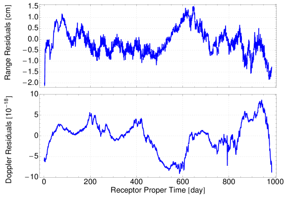
Figure 1: Representation of the Range (top) and Doppler (bottom) residuals for a simulation done in GR followed by a least-squares fit of the initial conditions using a GR model. These residuals are only due to numerical error. The orders of magnitude of the signals are $10^{9}$ km for the Range and $10^{-4}$ for the Doppler which means that the relative accuracy of the software is around $10^{-13}-10^{-14}$. This simulation has been performed for a two-way link to the Cassini spacecraft starting from May 2001.

5 Simulations in alternative theories of gravity

In this section, we present results obtained with our software (see also [62, 63]). The situation considered is the Cassini 3-years cruise from Jupiter to Saturn. We take the planetary initial conditions from ephemerides and the Cassini initial conditions from the SPICE and simulate a Range and a two-way Doppler link between Earth and Cassini spacecraft. We do not use any real data coming from the Cassini mission. Instead, we produce data in alternative theories of gravity and analyze them in GR in order to compare the expected deterministic signature in the (simulated) residuals with the Cassini precision. The simplified situation considered is the following: the Sun, the Earth and the Cassini spacecraft. We will show below that the addition of another planet (Jupiter for example) does not change significantly the results.

The correct analysis in GR is to fit initial conditions (eg. Earth and spacecraft positions/velocities, sun mass, etc…) to the simulated data, then the residuals of the fit (green continuous lines on figures 2, 3 and 7) are the incompressible physically observable signals expected in the residuals of the real data if the theory of gravity in nature is not GR (eg. PEG with $\delta\gamma=10^{-5}$ in figure 2, PEG with $\chi_{1}=10^{-21}\ m^{-1}$ in figure 3 or with an External Field Effect in figure 7). An alternative could be to not fit initial conditions in the GR analysis, but use the same initial conditions as in the simulation. The result then represents the difference in observables when starting from the same initial conditions but using different theories, and can give rise to signatures which are significantly larger than when fitting initial conditions (illustrated by the blue dash-dot curves on figures 2, 3 and 7), as the fit of initial conditions always absorbs some of the signal. We show these curves for illustration of that difference, but stress that drawing conclusions from these curves as to the expected signatures in the residuals of a real GR data analysis is incorrect, as in reality it is always necessary to fit initial conditions (they are unknown a priori).

Moreover, we only focus on two alternative theories of gravity presented in section 2: PEG theory and MOND EFE. In each of the simulations presented below, only one of the PEG and MOND EFE parameters is not vanishing. A more general study considering variations of several parameters is postponed to future work.

5.1 Simulations in Post-Einsteinian Gravity (PEG)

We use the metric (1a-1b) with the expansion of the potentials (1ba-1bb) to determine effects due to PEG on the Cassini signals. As can be seen from the expression of the metric (1a-1b), only corrections coming from the central body (the Sun) are considered, because these provide the most dominant contribution in the signature of the residuals. Different simulations were performed with different values of the PEG parameters and then analyzed in GR by fitting the initial conditions of the Earth, the initial conditions of Cassini spacecraft and the Sun mass. For example, figure 2 represents the Range and Doppler differences between a simulation in a theory with $\delta\gamma=\gamma-1=10^{-5}$ (and all other PEG parameters vanishing) and in GR. The three peaks occur during solar conjunctions. The blue (dash-dot) curves are the direct differences of signals generated in PEG theory with signals generated in GR. On the other hand, the green (continuous) lines represent the residuals obtained from simulated data in the alternative theory after the fit of the initial conditions. These signals are the ones expected to be detected in the residuals of the analysis of the real data if the theory of gravity is PEG theory (with $\delta\gamma=10^{-5}$) and if the analysis is performed with traditional GR theory.

On figure 2, we can see that the signal due to the conjunction is not absorbed at all by the fit of the initial conditions which nevertheless absorbs modulations between the conjunctions. Another example is given in figure 3 where the influence of a linear term in the spatial part of the metric is shown. As can be seen, in this case, the fit of the initial conditions absorbs a big part of the signal (the signal is absorbed by a factor 100).

In order to illustrate that the simplified situation considered here is sufficient to obtain correct residual templates, we performed simulations by adding Jupiter. figure 4 represents the difference between the residuals obtained by taking into account Jupiter and without the giant planet in the PEG simulation and in the GR analysis. Comparing the order of magnitude of figure 3 and figure 4, we can see that the addition of Jupiter does not change the residuals by more than roughly 5 %.

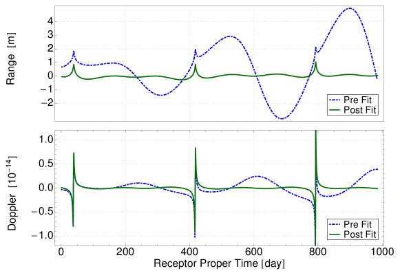
Figure 2: Representation of the Range (top) and Doppler (bottom) signals due to an alternative theory with $\gamma-1=10^{-5}$ (and all other PEG parameters vanishing). The blue (dash-dot) line is the difference between a simulation in the alternative theory and a simulation in GR (with the same initial conditions) and is for illustration purposes only (see text at the beginning of section 5). The green (continuous) line is the residuals obtained after analyzing the simulated data in GR (which means after the fit of the different initial conditions using a GR model) and represents the expected physical signal.

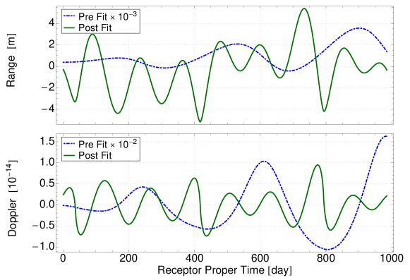
Figure 3: Representation of the Range (top) and Doppler (bottom) signals due to an alternative theory with $\chi_{1}=10^{-21}\ m^{-1}$ (and all other PEG parameters vanishing). The blue (dash-dot) line is the difference between a simulation in the alternative theory and a simulation in GR (with the same initial conditions) and is for illustration purposes only (see text at the beginning of section 5). The green (continuous) line is the residuals obtained after analyzing the simulated data in GR (which means after the fit of the different initial conditions using a GR model) and represents the expected physical signal.

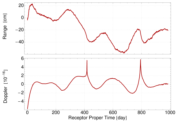
Figure 4: Representation of the difference of the Range (top) and Doppler (bottom) residuals between residuals computed with and without the presence of Jupiter for an alternative theory with $\chi_{1}=10^{-21}\ m^{-1}$ (and all other PEG parameters vanishing). The order of magnitude has to be compared with the order of magnitude of the residuals (green continuous lines) presented in figure 3: the presence of Jupiter changes the residuals obtained by only few %.

Figure 5 represents the residuals obtained for each PEG parameter considered. These are the signatures that need to be searched for systematically in the residuals of the GR analysis of real satellite data. Figure 6 summarizes all the simulations done. These figures represent the maximal difference between the Doppler generated in different PEG theories and the Doppler generated in GR. The different PEG theories are characterized by the values of their six parameters $\alpha_{1}$, $\alpha_{2}$, $\Lambda$, $\chi_{1}$, $\chi_{2}$, $\delta\gamma$. The blue (dash-dot) lines represent the maximal differences between simulations in PEG theory and simulations in GR with the same initial conditions. The green (continuous) lines represent the maximal residuals obtained after analyzing the signal generated in PEG theory in GR (i.e. after the fit of the initial conditions). More precisely, the green lines represent the maximal Doppler signal that we expect to see in the Cassini residuals if the theory of gravity is PEG theory with the considered parameters. Assuming a Cassini Doppler precision of roughly $10^{-14}$ (represented by the red (dashed) curves on figure 6), we derive the order of magnitude of the uncertainties one would obtain on the parameters of the theory when carrying out a search on the residuals from a complete GR analysis of real data. These uncertainties are given in table 1. Were one of these six PEG parameters larger than the value indicated in the table, a signal larger than Cassini precision would appear in the Doppler residuals (under the assumption that the signal is not completely absorbed by a fit of additional parameters of effects that are not considered here (eg. thermal radiation, solar pressure,…). . Clearly, a complete realistic data analysis would be necessary if an anomalous signal showed up with the right signature in the data. Then, a refined treatment taking into account the temporal signature of the signals and the spectral signature would be necessary. The boundary obtained on $\gamma$ is of the same order of magnitude as the one obtained by Bertotti et al [3] with the analysis of the real data ($\gamma-1=(2.1\pm 2.3)\times 10^{-5}$). The other values are completely new. It is also interesting to note that the boundary value on $\Lambda$ is of the order of $10\ kpc$ which corresponds to the galactic distance.

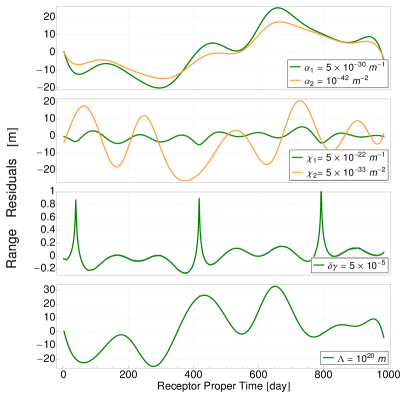
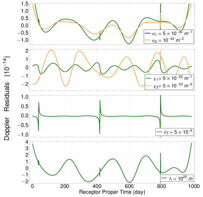
Figure 5: Representation of the Range (left) and Doppler (right) residuals for all the PEG parameters considered. These residuals are anomalous signals produced if the gravitation theory is PEG but if the data were analyzed in GR. These templates can be searched in residuals of an analysis of real data.

	smaller than
$\alpha_{1}$	$1.9\times 10^{-30}\ m^{-1}=5.9\times 10^{-11}\ kpc^{-1}$
$\alpha_{2}$	$6.2\times 10^{-43}\ m^{-2}=5.9\times 10^{-4}\ \ kpc^{-2}$
$\Lambda^{-1}$	$2.6\times 10^{-21}\ m^{-1}=0.08\ kpc^{-1}$
$\chi_{1}$	$5.3\times 10^{-22}\ m^{-1}=0.02\ kpc^{-1}$
$\chi_{2}$	$1.9\times 10^{-33}\ m^{-2}=1.8\times 10^{6}\ kpc^{-2}$
$\delta\gamma$	$3.7\times 10^{-5}$

Table 1: Estimate of the uncertainties on the six PEG parameters considered in this paper obtainable in a complete analysis with real data. These values are obtained by requesting the maximal residuals generated by the alternative theory to be smaller than the assumed Cassini Doppler precision. In the computation of these values, we vary only one parameter at a time independently of the others (set to zero).

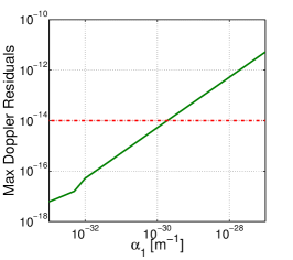
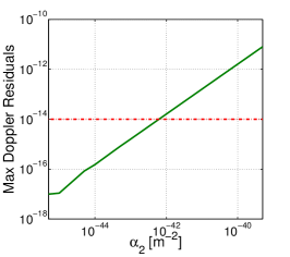
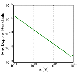
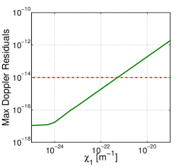
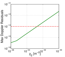
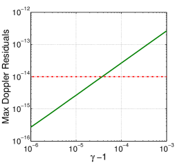
Figure 6: Representation of the maximal Doppler signal due to PEG theory (parameterized by the 6 parameters as indicated by the expansion (1ba-1bb) for the Cassini mission between Jupiter and Saturn. The green (continuous) lines represent the maximum residuals obtained after analyzing the simulated data in GR (i.e. after the fit of the initial conditions). The red (dashed) lines represent the assumed Cassini precision. Each subfigure represents the maximum of the Doppler residuals with respect to one PEG parameter (with all other PEG parameters vanishing).

5.2 Simulations with MOND external field effect

To analyze the influence of the MOND EFE, we use the metric (1a-1b) with the modifications of the potentials given by (1bea). Figure 7 represents the Range and Doppler difference between a simulation including MOND EFE (with the maximum value of the quadrupole allowed $Q_{2}=4.1\times 10^{-26}\ s^{-2}$) and a pure GR simulation. The residuals are too small to be detected with the considered arc of the Cassini mission. For this reason, the Cassini radioscience experiment (when the cruise was between Jupiter and Saturn) is not sensitive enough to the MOND EFE. However, it may well be visible with a longer arc of data, or when combining arcs from several spacecraft and possibly planetary observations. This will be the subject of future work. Finally, let us recall that the MOND EFE is very well constrained by the planetary ephemerides as indicated in section 2.

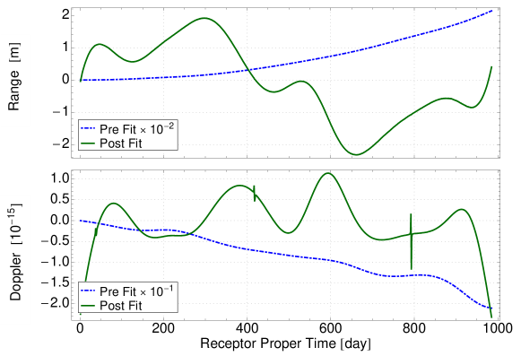
Figure 7: Representation of the Range (top) and Doppler (bottom) signals due to the MOND external field effect with $Q_{2}=4.1\times 10^{-26}\ s^{-2}$. The blue (dash-dot) line is the difference between a simulation in the alternative theory and a simulation in GR (with the same initial conditions) and is for illustration purposes only (see text at the beginning of section 5). The green (continuous) line is the residuals obtained after analyzing the simulated data in GR (which means after the fit of the different initial conditions) and represents the expected physical signal.

6 Conclusion

It is still an important challenge to test GR in the Solar System. Here, we focussed on the possibility to test GR with radioscience measurements. As emphasized in the introduction, it is essential to test GR in regimes not yet explored. This means looking either for deviations smaller than the current constraints (for example on the Post Newtonian Parameters) or for deviations in a more general framework than the ones used until today (mainly the PPN and the fifth force frameworks).

The work presented in this paper part of a project whose goal is to scan data from solar system observations for eventual violations of GR. Once completed, the full procedure will consist of four steps: simulations of observables in an alternative theory of gravity considering a simplified situation where only elements producing significant deviations from GR are simulated; analysis of these simulated observables using the usual procedure in GR to obtain the incompressible residuals due to the theory considered [32]; analysis of the real data using standard procedure in GR (including all known systematic effects); systematical search of the residuals of step (iii) using the template obtained in step (ii). In this paper, we have focussed on the two first steps. In particular, concerning the first step, we have presented a software aiming at simulating Range/Doppler observables directly from the space-time metric. This tool makes it easy to change the theory of gravity (the only thing to change is the metric). The method used to simulate Range and Doppler from the metric has been presented into detail. Moreover, concerning the second step of the procedure, we have used a software doing a simplified version of the traditional analysis in GR by means of a least-square fit of the different initial conditions involved in the problem.

While being very general, this approach has some limitations which are nevertheless justified since we are considering only the leading terms in the deviation from GR. Therefore, the gravitating bodies (Sun and Earth) are approximated as point masses. Note that if necessary, multipolar expansions could be taken into account. Nevertheless, the impact due to a modification of the gravitation theory on the multipolar expansion should be negligible (the effect of an alternative theory on the monopole term is already expected to be small). Considering point masses also means we suppose the observer to be located at the center of the Earth. The second simplification done is to neglect effects coming from a hypothetical violation of the Strong Equivalence Principle (SEP). A violation of the SEP implies a Nordtvedt term (parameterized by the Nordtvedt parameter $\eta$) in the equations of motion [64, 65] which can be added in the software if necessary. Finally, an implicit assumption done using the least-squares fit is that the error distribution of the measurements to be Gaussian.

Our results correspond to simulations in two alternative theories of gravity: Post-Einsteinian Gravity and the External Field Effect due to a MOND theory of gravity. The simulations have been performed for the Cassini spacecraft during its cruise between Jupiter and Saturn. The Range and Doppler residuals due to these theories have been presented in figure 5. These residuals furnished templates for signatures that can be searched for in real data analysis. The parameters uncertainties reachable in a complete analysis with real data have been estimated and are given in table 1.

The External Field Effect due to a MOND theory of gravity on the considered arc of the Cassini mission is just too small to be observed. This arc can not give a significant constraint on the MOND theory, astrometric data based on perihelia precessions giving better constraints [4].

Let us summarize the innovative points of this work. The approach followed by deriving radioscience signals from the space-time metric is very general and makes it possible to obtain observables in alternative theories of gravity independently from the coordinate systems used and independently from any exterior data treated in GR (for example without any reference to ephemerides computed in GR). The fit of the initial conditions which is quite often forgotten in the analysis of anomalies can reduce the deviations produced in the observables quite significantly depending on the theory considered. A first crude limit on PEG parameters can be derived by using the Cassini spacecraft. Finally, this software can be used to test other alternative theories of gravity.

The method presented here can be generalized to non metric theories provided the equations of motion of massive bodies and the equations of light propagation are known. In general, these equations can be derived from the field equations. Simulations in nearly every alternative theory of gravity (for example Standard Model Extension, TeVeS, …) can thus be made. Another perspective is to extend the software to simulate observations related to angular measurements (VLBI, position of star in the sky, position of planets) which constitutes the other type of measurement done in the Solar System. Such an extension will allow one to simulate all the observations done in the Solar System in any metric theory of gravity and to derive the expected signals in the residuals when analyzing those observables in GR.

Finally, radioscience data from existing and future space missions could be analyzed to derive more precise constraints on alternative theories of gravity.

References

References

- [1] C. M. Will. Theory and Experiment in Gravitational Physics. March 1993.
- [2] C. M. Will. The Confrontation between General Relativity and Experiment. Living Reviews in Relativity, 9:3, March 2006.
- [3] B. Bertotti, L. Iess, and P. Tortora. A test of general relativity using radio links with the Cassini spacecraft. Nature, 425:374–376, September 2003.
- [4] A. Fienga, J. Laskar, P. Kuchynka, H. Manche, G. Desvignes, M. Gastineau, I. Cognard, and G. Theureau. The INPOP10a planetary ephemeris and its applications in fundamental physics. Celestial Mechanics and Dynamical Astronomy, 111(3):363–385, September 2011.
- [5] J. G. Williams, S. G. Turyshev, and D. H. Boggs. Lunar Laser Ranging Tests of the Equivalence Principle with the Earth and Moon. International Journal of Modern Physics D, 18:1129–1175, 2009.
- [6] A. S. Konopliv, S. W. Asmar, W. M. Folkner, Ö. Karatekin, D. C. Nunes, S. E. Smrekar, C. F. Yoder, and M. T. Zuber. Mars high resolution gravity fields from mro, mars seasonal gravity, and other dynamical parameters. Icarus, 211(1):401 – 428, 2011.
- [7] E. G. Adelberger, B. R. Heckel, and A. E. Nelson. Tests of the Gravitational Inverse-Square Law. Annual Review of Nuclear and Particle Science, 53:77–121, December 2003.
- [8] E. G. Adelberger, J. H. Gundlach, B. R. Heckel, S. Hoedl, and S. Schlamminger. Torsion balance experiments: A low-energy frontier of particle physics. Progress in Particle and Nuclear Physics, 62:102–134, January 2009.
- [9] C. Talmadge, J.-P. Berthias, R. W. Hellings, and E. M. Standish. Model-independent constraints on possible modifications of Newtonian gravity. Physical Review Letters, 61:1159–1162, September 1988.
- [10] E. Fischbach and C. L. Talmadge. The Search for Non-Newtonian Gravity. Aip-Press Series. Springer, 1999.
- [11] J. D. Anderson, P. A. Laing, E. L. Lau, A. S. Liu, M. M. Nieto, and S. G. Turyshev. Indication, from Pioneer 10/11, Galileo, and Ulysses Data, of an Apparent Anomalous, Weak, Long-Range Acceleration. Physical Review Letters, 81:2858–2861, October 1998.
- [12] J. D. Anderson, P. A. Laing, E. L. Lau, A. S. Liu, M. M. Nieto, and S. G. Turyshev. Study of the anomalous acceleration of Pioneer 10 and 11. Phys. Rev. D, 65(8):082004, April 2002.
- [13] A. Levy, B. Christophe, P. Bério, G. Métris, J.-M. Courty, and S. Reynaud. Pioneer 10 Doppler data analysis: Disentangling periodic and secular anomalies. Advances in Space Research, 43:1538–1544, May 2009.
- [14] S. G. Turyshev and V. T. Toth. The Pioneer Anomaly. Living Reviews in Relativity, 13:4, September 2010.
- [15] S. G. Turyshev, V. T. Toth, J. Ellis, and C. B. Markwardt. Support for Temporally Varying Behavior of the Pioneer Anomaly from the Extended Pioneer 10 and 11 Doppler Data Sets. Physical Review Letters, 107(8):081103, August 2011.
- [16] S. G. Turyshev, V. T. Toth, G. Kinsella, S.-C. Lee, S. M. Lok, and J. Ellis. Support for the thermal origin of the Pioneer anomaly. Physical Review Letters, 108(24):241101, June 2012.
- [17] T. Damour and K. Nordtvedt. Tensor-scalar cosmological models and their relaxation toward general relativity. Phys. Rev. D, 48:3436–3450, October 1993.
- [18] T. Damour and K. Nordtvedt. General relativity as a cosmological attractor of tensor-scalar theories. Physical Review Letters, 70:2217–2219, April 1993.
- [19] J. Khoury and A. Weltman. Chameleon cosmology. Phys. Rev. D, 69(4):044026, February 2004.
- [20] J. Khoury and A. Weltman. Chameleon Fields: Awaiting Surprises for Tests of Gravity in Space. Phys. Rev. Lett., 93(17):171104, October 2004.
- [21] A. Hees and A. Füzfa. Combined cosmological and solar system constraints on chameleon mechanism. Phys. Rev. D, 85(10):103005, May 2012.
- [22] M.-T. Jaekel and S. Reynaud. Post-Einsteinian tests of linearized gravitation. Classical and Quantum Gravity, 22:2135–2157, June 2005.
- [23] M.-T. Jaekel and S. Reynaud. Gravity Tests in the Solar System and the Pioneer Anomaly. Modern Physics Letters A, 20:1047–1055, 2005.
- [24] M.-T. Jaekel and S. Reynaud. Post-Einsteinian tests of gravitation. Classical and Quantum Gravity, 23:777–798, February 2006.
- [25] M.-T. Jaekel and S. Reynaud. Radar ranging and Doppler tracking in post-Einsteinian metric theories of gravity. Classical and Quantum Gravity, 23:7561–7579, December 2006.
- [26] S. Reynaud and M.-T. Jaekel. Long Range Gravity Tests and the Pioneer Anomaly. International Journal of Modern Physics D, 16:2091–2105, 2007.
- [27] T. Faulkner, M. Tegmark, E. F. Bunn, and Y. Mao. Constraining f(R) gravity as a scalar-tensor theory. Phys. Rev. D, 76(6):063505, September 2007.
- [28] S. Capozziello and S. Tsujikawa. Solar system and equivalence principle constraints on f(R) gravity by the chameleon approach. Phys. Rev. D, 77(10):107501, May 2008.
- [29] A. de Felice and S. Tsujikawa. f(R) Theories. Living Reviews in Relativity, 13(3), June 2010.
- [30] Quentin G. Bailey and V. Alan Kostelecký. Signals for lorentz violation in post-newtonian gravity. Phys. Rev. D, 74:045001, Aug 2006.
- [31] Quentin G. Bailey. Time delay and doppler tests of the lorentz symmetry of gravity. Phys. Rev. D, 80:044004, Aug 2009.
- [32] O. Zarrouati. Trajectoires spatiales. Editions Cépaduès, 1987.
- [33] L. Blanchet and J. Novak. External field effect of modified Newtonian dynamics in the Solar system. MNRAS, 412:2530–2542, April 2011.
- [34] L. Blanchet and J. Novak. Testing MOND in the Solar System. In E. Augé, J. Dumarchez, and J. Trân Thanh Vân, editors, Proceedings of the XLVIth Rencontres de Moriond and GPhys Colloquium 2011: Gravitational Waves and Experimental Gravity, page 295, Vietnam, May 2011. Thê Giói Publishers.
- [35] B. Lamine, J. M. Courty, S. Reynaud, and M. T. Jaekel. Testing gravity law in the solar system. In N. Capitaine, editor, Proceedings of the Journées 2010 ”Systèmes de Référence Spatio-Temporels”. Observatoire de Paris, May 2011.
- [36] P. D. Mannheim and D. Kazanas. Exact vacuum solution to conformal Weyl gravity and galactic rotation curves. ApJ, 342:635–638, July 1989.
- [37] J. E. Tohline. Stabilizing a cold disk with a 1/r force law. In E. Athanassoula, editor, Internal Kinematics and Dynamics of Galaxies, volume 100 of IAU Symposium, page 205, 1983.
- [38] J. R. Kuhn and L. Kruglyak. Non-Newtonian forces and the invisible mass problem. ApJ, 313:1–12, February 1987.
- [39] F. W. Hehl and B. Mashhoon. Formal framework for a nonlocal generalization of Einstein’s theory of gravitation. Phys. Rev. D, 79(6):064028, March 2009.
- [40] M. Milgrom. A modification of the Newtonian dynamics as a possible alternative to the hidden mass hypothesis. ApJ, 270:365–370, July 1983.
- [41] M. Milgrom. MOND effects in the inner Solar system. MNRAS, 399:474–486, October 2009.
- [42] M. H. Soffel. Relativity in Astrometry, Celestial Mechanics and Geodesy. 1989.
- [43] V. A. Brumberg. Essential relativistic celestial mechanics. Adam Hilger, 1991.
- [44] C. W. Misner, K. S. Thorne, and J. A. Wheeler. Gravitation. Physics Series. W. H. Freeman, 1973.
- [45] A. Hees and S. Pireaux. A relativistic motion integrator: numerical accuracy and illustration with BepiColombo and Mars-NEXT. In S. A. Klioner, P. K. Seidelmann, & M. H. Soffel, editor, IAU Symposium, volume 261 of IAU Symposium, pages 144–146, January 2010.
- [46] A. Fienga, J. Laskar, T. Morley, H. Manche, P. Kuchynka, C. Le Poncin-Lafitte, F. Budnik, M. Gastineau, and L. Somenzi. INPOP08, a 4-D planetary ephemeris: from asteroid and time-scale computations to ESA Mars Express and Venus Express contributions. A&A, 507:1675–1686, December 2009.
- [47] X. X. Newhall, E. M. Standish, and J. G. Williams. DE 102 - A numerically integrated ephemeris of the moon and planets spanning forty-four centuries. A&A, 125:150–167, August 1983.
- [48] E. V. Pitjeva. High-Precision Ephemerides of Planets EPM and Determination of Some Astronomical Constants. Solar System Research, 39:176–186, May 2005.
- [49] A. Fienga, J. Laskar, P. Kuchynka, C. Le Poncin-Lafitte, H. Manche, and M. Gastineau. Gravity tests with INPOP planetary ephemerides. In S. A. Klioner, P. K. Seidelmann, & M. H. Soffel, editor, IAU Symposium, volume 261 of IAU Symposium, pages 159–169, January 2010.
- [50] W. M. Folkner. Relativistic aspects of the JPL planetary ephemeris. In S. A. Klioner, P. K. Seidelmann, & M. H. Soffel, editor, IAU Symposium, volume 261 of IAU Symposium, pages 155–158, January 2010.
- [51] E. V. Pitjeva. EPM ephemerides and relativity. In S. A. Klioner, P. K. Seidelmann, & M. H. Soffel, editor, IAU Symposium, volume 261 of IAU Symposium, pages 170–178, January 2010.
- [52] C. Le Poncin-Lafitte, B. Linet, and P. Teyssandier. World function and time transfer: general post-Minkowskian expansions. CQG, 21:4463–4483, September 2004.
- [53] P. Teyssandier and C. Le Poncin-Lafitte. General post-Minkowskian expansion of time transfer functions. CQG, 25:145020, July 2008.
- [54] G. Petit and P. Wolf. Relativistic theory for picosecond time transfer in the vicinity of the Earth. Astron. Astrophys., 286:971–977, June 1994.
- [55] A. San Miguel. Numerical determination of time transfer in general relativity. General Relativity and Gravitation, 39:2025–2037, December 2007.
- [56] L. Blanchet, C. Salomon, P. Teyssandier, and P. Wolf. Relativistic theory for time and frequency transfer to order . A&A, 370:320–329, April 2001.
- [57] C. F. Peters. Numerical integration of the satellites of the outer planets. Astron. Astrophys., 104:37–41, December 1981.
- [58] V. Lainey, L. Duriez, and A. Vienne. New accurate ephemerides for the Galilean satellites of Jupiter. I. Numerical integration of elaborated equations of motion. A&A, 420:1171–1183, June 2004.
- [59] V. Lainey, J. E. Arlot, and A. Vienne. New accurate ephemerides for the Galilean satellites of Jupiter. II. Fitting the observations. A&A, 427:371–376, November 2004.
- [60] M. Soffel, S. A. Klioner, G. Petit, P. Wolf, S. M. Kopeikin, P. Bretagnon, V. A. Brumberg, N. Capitaine, T. Damour, T. Fukushima, B. Guinot, T.-Y. Huang, L. Lindegren, C. Ma, K. Nordtvedt, J. C. Ries, P. K. Seidelmann, D. Vokrouhlický, C. M. Will, and C. Xu. The IAU 2000 Resolutions for Astrometry, Celestial Mechanics, and Metrology in the Relativistic Framework: Explanatory Supplement. Astronomical Journal, 126:2687–2706, December 2003.
- [61] C. Bonanno and A. Milani. Symmetries and Rank Deficiency in the Orbit Determination Around Another Planet. Celestial Mechanics and Dynamical Astronomy, 83:17–33, May 2002.
- [62] A. Hees, P. Wolf, B. Lamine, S. Reynaud, M.-T. Jaekel, C. Le Poncin-Lafitte, V. Lainey, A. Füzfa, and V. Dehant. Radioscience simulations in General Relativity and in alternative theories of gravity. In E. Augé, J. Dumarchez, and J. Trân Thanh Vân, editors, Proceedings of the XLVIth Rencontres de Moriond and GPhys Colloquium 2011: Gravitational Waves and Experimental Gravity, page 259, Vietnam, May 2011. Thê Giói Publishers.
- [63] A. Hees, P. Wolf, B. Lamine, S. Reynaud, M. T. Jaekel, C. Le Poncin-Lafitte, V. Lainey, and V. Dehant. Testing gravitation in the Solar System with radio science experiments. In G. Alecian, K. Belkacem, R. Samadi & D. Valls-Gabaud, editor, SF2A-2011: Proceedings of the Annual meeting of the French Society of Astronomy and Astrophysics, pages 653–658, December 2011.
- [64] K. Nordtvedt. Equivalence Principle for Massive Bodies. I. Phenomenology. Physical Review, 169:1014–1016, May 1968.
- [65] K. Nordtvedt. Equivalence Principle for Massive Bodies. II. Theory. Physical Review, 169:1017–1025, May 1968.