The motion of the 2D hydrodynamic Chaplygin sleigh
in the presence of circulation

Abstract

We consider the motion of a planar rigid body in a potential flow with circulation and subject to a certain nonholonomic constraint. This model is related to the design of underwater vehicles.

The equations of motion admit a reduction to a 2-dimensional nonlinear system, which is integrated explicitly. We show that the reduced system comprises both asymptotic and periodic dynamics separated by a critical value of the energy, and give a complete classification of types of the motion. Then we describe the whole variety of the trajectories of the body on the plane.

1 Introduction and outline

In this paper, we consider the motion of a planar rigid body surrounded by an irrotational perfect fluid. It ia assumed that there is a given amount $\kappa$ of circulation around the body, and that the body is subject to a certain nonholonomic constraint, which models a very effective keel or fin attached to the body. In the absence of circulation this system was termed the hydrodynamic Chaplygin sleigh in [11], since in the absence of the fluid, the nonholonomic constraint models the effect of a sharp blade in the classical Chaplygin sleigh problem [7] which prevents the sleigh from moving in the lateral direction.

The hydrodynamic Chaplygin sleigh in the presence of circulation was recently considered in [12], where it was shown that it is an LL system on a certain central extension of $SE(2)$ by $\mathbb{R}^{3}$, where the cocycle encodes the effects of the circulation on the body.

Our model for the nonholonomic constraint, which respects the Lagrange-D’Alembert principle, has been considered in the aerospace engineering community [23], while robotic models for underwater vehicles taking into account the effects of circulation were considered in [15].

History of the Kirchhoff equations.

The motion of a rigid body in a potential fluid in the absence of external forces was first described by Kirchhoff [16]. His crucial observation was that the effect of the fluid on the body could be described entirely in terms of the added mass and added inertia terms, which depend on the geometry of the body only, and can be calculated analytically for a wide class of body shapes. Kirchhoff’s solution was extended to the case of rigid bodies moving in potential flow with circulation by, among others, Chaplygin [6] and [17], who derived the equations of motion for this system, provided an explicit integration in terms of elliptic functions, and described qualitative features of the dynamics, such as periodic motions. In recent years, these ideas have been extended to the case of rigid bodies interacting with point vortices [26, 2], vortex rings [27] and other vortical structures, and they have been used to describe underwater vehicles [18] and the motion of bio-organisms [4, 5]. A comprehensive overview of the history of these equations can be found in [3].

Contributions of this paper.

We show that the hydrodynamic Chaplygin sleigh with circulation is a new example of a completely integrable nonholonomic system: we discuss qualitative features of the dynamics, and we explicitly integrate the reduced equations of motion.

Contents of the paper.

In section 2 we recall Kirchhoff’s equations for a planar rigid body moving in a potential fluid and consider the Chaplygin-Lamb equations for the motion of the body in the presence of circulation. For the purpose of completeness, the added masses are computed explicitly for a body of elliptical shape.

In section 3, the reduced equations of motion on the coalgebra $se(2)^{*}$ are written explicitly in terms of the added masses and the coefficient $\alpha$ that depends on the position and orientation of the fin (or blade) on the body. Again, for the purpose of completeness, we give explicit formulas for the parameters that enter the equations for a body having an elliptical shape. It is shown that the presence of circulation around the body adds new features to the motion of the hydrodynamic Chaplygin sleigh, and that there exists a critical value of the kinetic energy of the fluid-body system that divides periodic from asymptotic behavior. Indeed, for small, subcritical energy values, the reduced dynamics are periodic. In this case the circulation effects drive the dynamics (via the so-called Kutta-Zhukowski force). On the contrary, if the initial energy is supercritical, then the inertia of the body overcomes the circulation effects and it evolves asymptotically from one circular motion to another, where the limit circumferences have different radius. This resembles the motion of the body in the absence of circulation treated in [11]. Moreover, we identify 7 regions in the reduced phase space that yield distinct qualitative dynamics of the motion of the sleigh on the plane.

In section 4 the reduced equations of motion for the hydrodynamic Chaplygin sleigh with circulation are integrated explicitly for a generic sleigh. The form of the solution varies according to the energy regime. If the energy is subcritical, the solution is a quotient of trigonometric functions and we give an explicit expression for the period in terms of the energy. We also give a closed expression for the angular part of the monodromy matrix that is involved in the reconstruction process. This formula allows us to show that the qualitative behavior of the sleigh on the plane is very sensitive to initial conditions for energy values that are slightly subcritical.

On the other hand, for the critical value of the energy, the solution of the reduced equations is given as a rational function of time. The closed expression for the solution is used to show that the motion of the sleigh on the plane in this case is bounded and evolves from one circular motion to another, where the limit circumferences have equal radius. Finally, the solution of the reduced equations for supercritical energies is given as a quotient of hyperbolic functions. In this case we also express the distance between the centers of the limit circumferences in terms of integrals generalizing the Beta-function.

In Conclusions we motivate a further study of the hydrodynamic Chaplygin sleigh in the presence of point vortices.

2 Preliminaries: Fluid-structure interactions

In this section, we give an overview of the Kirchhoff equations describing the dynamics of a rigid body in potential flow, and of the Chaplygin-Lamb equations dealing with rigid bodies in the presence of circulation. Most of the material covered in this section can be found, for instance, in [14] as well as in the classical works of Lamb [17] and Milne-Thomson [20].

2.1 Kinematics of rigid bodies and ideal fluids

Following Euler’s approach, consider an orthonormal body frame $\{{\bf E}_{1},{\bf E}_{2}\}$ that is attached to the body. This frame is related to a fixed space frame $\{{\bf e}_{1},{\bf e}_{2}\}$ by a rotation by an angle $\theta$ that specifies the orientation of the two dimensional body at each time. We will denote by ${\bf x}=(x,y)\in\mathbb{R}^{2}$ the spatial coordinates of the origin of the body frame (see Figure 1). The configuration of the body at any time is completely determined by the element $g$ of the two dimensional Euclidean group $SE(2)$ given by

$$g=\left(\begin{array}[]{ccc}\cos\theta&-\sin\theta&x\\ \sin\theta&\cos\theta&y\\ 0&0&1\end{array}\right)\in SE(2).$$

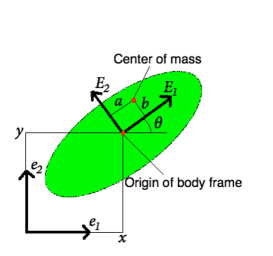
(a) Body frame is aligned with axes of symmetry of the body

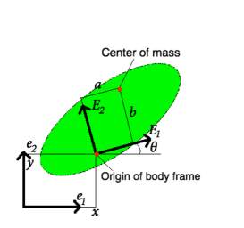
(b) Arbitrary position and orientation of the body frame.

Figure 1: Two different choices of the body frame for an elliptical two-dimensional rigid body. In both cases the origin of the body frame does not coincide with the center of mass.

We will often denote the above element in $g\in SE(2)$ by $g=(R_{\theta},{\bf x})$ where $R_{\theta}\in\operatorname{SO}(2)$ is the rotation matrix determined by the angle $\theta$. Let $(v_{1},v_{2})\in\mathbb{R}^{2}$ be the linear velocity of the origin of the body frame written in the body coordinates, and denote by $\omega=\dot{\theta}$ the body’s angular velocity. They define the element $\xi$ in the Lie algebra $se(2)$ given by

$$\xi=g^{-1}\dot{g}=\left(\begin{array}[]{ccc}0&-\omega&v_{1}\\ \omega&0&v_{2}\\ 0&0&0\end{array}\right)\in se(2).$$

Explicitly we have

$$\dot{\theta}=\omega,\qquad v_{1}=\dot{x}\cos\theta+\dot{y}\sin\theta,\quad v_{2}=-\dot{x}\sin\theta+\dot{y}\cos\theta.$$ (2.1)

For convenience, we will sometimes denote $\xi\in se(2)$ as the column vector $(\omega,v_{1},v_{2})^{T}\in\mathbb{R}^{3}$. The Lie algebra commutator takes the form

$$\left[\,(\omega,v_{1},v_{2})\,,\,(\omega^{\prime},v_{1}^{\prime},v_{2}^{\prime})\,\right]_{\mathfrak{se}(2)}=(\,0\,,\,v_{2}\omega^{\prime}-\omega v_{2}^{\prime}\,,\,\omega v_{1}^{\prime}-v_{1}\omega^{\prime}\,).$$

The kinetic energy of the body is given by

$$T_{\mathcal{B}}=\frac{1}{2}\left((\mathcal{I}_{\mathcal{B}}+ma^{2}+mb^{2})\omega^{2}+m(v_{1}^{2}+v_{2}^{2})-mb\omega v_{1}+ma\omega v_{2}\right),$$ (2.2)

where $m$ is the mass of the body, $(a,b)$ are body coordinates of the center of mass (see Figure 1), and $\mathcal{I}_{\mathcal{B}}$ is the moment of inertia of the body about the center of mass. It is a positive definite quadratic form on $se(2)$ whose matrix is the body inertia tensor

$$\mathbb{I}_{\mathcal{B}}=\left(\begin{array}[]{ccc}\mathcal{I}_{\mathcal{B}}+m(a^{2}+b^{2})&-mb&ma\\ -mb&m&0\\ ma&0&m\end{array}\right).$$ (2.3)

The fluid flow at a given instant.

Consider now the motion of the fluid that surrounds the body. Suppose that at a given instant the body occupies a region $\mathcal{B}\subset\mathbb{R}^{2}$. The flow is assumed to take place in the connected unbounded region $\mathcal{U}:=\mathbb{R}^{2}\setminus\mathcal{B}$ that is not occupied by the body.

We assume that the flow is potential so the Eulerian velocity of the fluid ${\bf u}$ can be written as ${\bf u}=\nabla\Phi$ for a fluid potential $\Phi:\mathcal{U}\to\mathbb{R}$. Incompressibility of the fluid implies that $\Phi$ is harmonic,

$$\nabla^{2}\Phi=0\qquad\mbox{on}\qquad\mathcal{U}.$$

The boundary conditions for $\Phi$ come from the following considerations. On the one hand it is assumed that, up to a purely circulatory flow around the body, the motion of the fluid is solely due to the motion of the body. This assumption requires the fluid velocity $\nabla\Phi$ to vanish at infinity. Secondly, to avoid cavitation or penetration of the fluid into the body, we require the normal component of the fluid velocity at a material point $p$ on the boundary of $\mathcal{B}$ to agree with the normal component of the velocity of $p$. Suppose that the vector $(X,Y)\in\mathbb{R}^{2}$ gives body coordinates for $p$. The latter boundary condition is expressed as

$$\left.\frac{\partial\Phi}{\partial n}\right|_{p\in\partial\mathcal{B}}=(v_{1}-\omega Y)n_{1}+(v_{2}+\omega X)n_{2},$$

where ${\bf n}=(n_{1},n_{2})$ is the outward unit normal vector to $\mathcal{B}$ at $p$ written in body coordinates. These conditions determine the flow of the fluid up to a purely circulatory flow around the body that would persist if the body is brought to rest. The latter is specified by the value of the circulation $\kappa$ around the body as we now discuss.

The potential $\Phi$ that satisfies the above boundary value problem can be written in terms of the body’s velocities $v_{1},v_{2},\omega$, in Kirchhoff form:

$$\Phi=v_{1}\phi_{1}+v_{2}\phi_{2}+\omega\chi+\phi_{0},$$ (2.4)

where $\phi_{i}$, $i=0,1,2$, and $\chi$ are harmonic functions on $\mathcal{U}$ whose gradients vanish at infinity and satisfy:

$$\left.\frac{\partial\phi_{i}}{\partial n}\right|_{\partial\mathcal{B}}=n_{i},\;i=1,2,\qquad\left.\frac{\partial\chi}{\partial n}\right|_{\partial\mathcal{B}}=Xn_{2}-Yn_{1},\qquad\left.\frac{\partial\phi_{0}}{\partial n}\right|_{\partial\mathcal{B}}=0.$$

The potential $\phi_{0}$ is multi-valued and defines the circulatory flow around the body. The circulation $\kappa$ of the fluid around the body satisfies

$$\kappa=\oint_{\partial\mathcal{B}}{\bf u}\cdot d{\mathbf{l}}=\oint_{\partial\mathcal{B}}\nabla\phi_{0}\cdot d{\mathbf{l}},$$

and remains constant during the motion. Figure 2 shows the streamline pattern of the flow determined by the motion of an elliptical body for different values of $\kappa$.

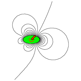
(a) $\kappa=0$

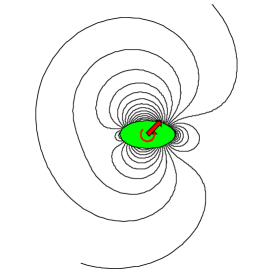
(b) $\kappa=2\pi$

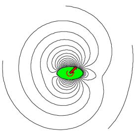
(c) $\kappa=10$

Figure 2: Stream line pattern for an ellipse moving on the plane for different values of the circulation $\kappa$. The major and minor semi-axes of the ellipse are $A=2,B=1$. The body frame is aligned with the principal axes of the ellipse and the velocity of the body satisfies $v_{1}=v_{2}=1$ and $\omega=5$.

Disregarding the circulatory motion, the kinetic energy of the fluid is given by

$$T_{\mathcal{F}}=\frac{\rho}{2}\int_{\mathcal{U}}||\nabla(\Phi-\phi_{0})||^{2}\,dA,$$

where $dA$ is the area element in $\mathbb{R}^{2}$ and $\rho$ is the (constant) fluid density. We have subtracted the circulatory part from the velocity potential, as it would give rise to an infinite contribution to the fluid kinetic energy [25].

By substituting (2.4) into the above, one can express $T_{\mathcal{F}}$ as the quadratic form

$$T_{\mathcal{F}}=\frac{1}{2}\left(\sum_{i,j=1}^{2}\mathcal{M}^{ij}_{\mathcal{F}}v_{i}v_{j}+2\sum_{i=1}^{2}\mathcal{K}^{i}_{\mathcal{F}}v_{i}\omega+\mathcal{I}_{\mathcal{F}}\omega^{2}\right),$$ (2.5)

where $\mathcal{M}_{\mathcal{F}}^{ij},\mathcal{K}_{\mathcal{F}}^{i}$, $i,j=1,2$, and $\mathcal{I}_{\mathcal{F}}$ are certain constants that only depend on the body shape. Explicitly one has (see [17] for details),

$$\begin{split}&\mathcal{M}^{ij}_{\mathcal{F}}=-\rho\int_{\partial\mathcal{B}}\phi_{i}\frac{\partial\phi_{j}}{\partial n}\,dl=-\rho\int_{\partial\mathcal{B}}\phi_{j}\frac{\partial\phi_{i}}{\partial n}\,dl,\;i,j=1,2,\qquad\mathcal{I}_{\mathcal{F}}=-\rho\int_{\partial\mathcal{B}}\chi\frac{\partial\chi}{\partial n}\,dl\\ &\mathcal{K}^{i}_{\mathcal{F}}=-\rho\int_{\partial\mathcal{B}}\phi_{i}\frac{\partial\chi}{\partial n}\,dl=-\rho\int_{\partial\mathcal{B}}\chi\frac{\partial\phi_{i}}{\partial n}\,dl,\;i=1,2.\end{split}$$

These constants are referred to as added masses and are conveniently written in $3\times 3$ matrix form to define the (symmetric) added inertia tensor:

$$\mathbb{I}_{\mathcal{F}}:=\left(\begin{array}[]{cc}\mathcal{I}_{\mathcal{F}}&\mathcal{K}_{\mathcal{F}}\\ \mathcal{K}_{\mathcal{F}}^{T}&\mathcal{M}_{\mathcal{F}}\end{array}\right),$$

that defines $T_{\mathcal{F}}$ as a quadratic form on $se(2)$.

• For an elliptic rigid body with semi-axes of length $A>B>0$, the added masses and moments of inertia take on a particularly convenient form. The kinetic energy of the fluid is given by (see [17])

  $$T_{\mathcal{F}}=\frac{\rho\pi}{2}\left(B^{2}v_{1}^{2}+A^{2}v_{2}^{2}+\frac{(A^{2}-B^{2})^{2}}{4}\omega^{2}\right),$$

  where we have ignored the circulatory motion around the body. The corresponding added inertia tensor is thus given by

  $$\mathbb{I}_{\mathcal{F}}=\rho\pi\left(\begin{array}[]{ccc}\frac{(A^{2}-B^{2})^{2}}{4}&0&0\\ 0&B^{2}&0\\ 0&0&A^{2}\end{array}\right).$$ (2.6)

  We emphasize that this particular form of the added inertia tensor was derived under the assumption that the body frame is aligned with the symmetry axes of the ellipse ($\nu=0$, $r=s=0$ in Figure 3 ahead). When this is not the case, the added mass tensor is more complicated, and in particular need not be diagonal, as is shown in (3.12).

2.2 Rigid body motion in potential flow

The total kinetic energy, $T$, of the solid-fluid system (excluding the circulatory motion) is the sum of the kinetic energy $T_{\mathcal{B}}$ of the rigid body and the energy $T_{\mathcal{F}}$ of the fluid. As both $T_{\mathcal{B}}$ and $T_{\mathcal{F}}$ are functions on $TSE(2)$, so is the total energy $T$. In the absence of external forces or circulation, the Lagrangian $\mathcal{L}$ of the solid-fluid system is just the kinetic energy: $\mathcal{L}=T$, and in this case, the motion of the rigid body describes a geodesic curve in $SE(2)$ with respect to the Riemannian metric defined by $\mathcal{L}$.

In view of (2.2) and (2.5), we can write the Lagrangian $\mathcal{L}=T_{\mathcal{B}}+T_{\mathcal{F}}$ in terms of the linear and angular velocities of the body (written in the body frame) and this expression does not depend on the particular position and orientation of the body, i.e. is independent of the group element $g=(R_{\theta},{\bf x})\in SE(2)$. Thus $\mathcal{L}$ is invariant under the lifted action of left multiplication on $SE(2)$. This symmetry corresponds to invariance under translations and rotations of the space frame. The reduction of this symmetry defines Euler-Poincaré equations on the Lie algebra $se(2)$ or, in the Hamiltonian setting, the Lie-Poisson equations on the coalgebra $se(2)^{*}$. The latter are precisely Kirchhoff’s equations that are explicitly written below.

The invariance of $\mathcal{L}$ allows us to define a function $L$ on $se(2)$, called the reduced Lagrangian. Explicitly, $L$ is given by

$$L(\xi)=\frac{1}{2}\xi^{T}\mathbb{I}\xi,$$

where $\xi=(\omega,v_{1},v_{2})^{T}\in se(2)\cong\mathbb{R}^{3}$ is a column vector and the matrix $\mathbb{I}$ is the sum of the inertia matrix $\mathbb{I}_{B}$ of the rigid body and the added masses and inertia $\mathbb{I}_{\mathcal{F}}$ of the fluid: $\mathbb{I}=\mathbb{I}_{\mathcal{B}}+\mathbb{I}_{\mathcal{F}}$.

Since $se(2)$ is isomorphic to $\mathbb{R}^{3}$ and using the Euclidian inner product, we identify $se(2)^{\ast}\cong\mathbb{R}^{3}$. A typical element $\mu$ is represented as a row vector $\mu=(k,p_{1},p_{2})$. The duality pairing between $\mu$ and an element $\xi=(\omega,v_{1},v_{2})^{T}$ of $se(2)$ is given by

$$\langle\mu,\xi\rangle=\mu\xi=k\omega+p_{1}v_{1}+p_{2}v_{2}.$$

With this identification, the Legendre transform associated to $L$ is defined as the mapping

$$\mathbb{F}L:se(2)\rightarrow se(2)^{\ast}$$

given by $\mathbb{F}L(\xi)=\mu$, where $\mu=(\mathbb{I}\xi)^{T}$. The components of $\mu=(k,p_{1},p_{2})$ are explicitly given by

$$\begin{split}k&=(\mathcal{I}_{\mathcal{B}}+m(a^{2}+b^{2})+\mathcal{I}_{\mathcal{F}})\omega+(-mb+\mathcal{K}_{\mathcal{F}}^{1})v_{1}+(ma+\mathcal{K}_{\mathcal{F}}^{2})v_{2},\\ p_{1}&=(-mb+\mathcal{K}_{\mathcal{F}}^{1})\omega+(m+\mathcal{M}^{11}_{\mathcal{F}})v_{1}+\mathcal{M}^{12}v_{2},\\ p_{2}&=(ma+\mathcal{K}_{\mathcal{F}}^{2})\omega+\mathcal{M}^{12}v_{1}+(m+\mathcal{M}^{22}_{\mathcal{F}})v_{2}.\end{split}$$ (2.7)

In classical hydrodynamics $k$ and $(p_{1},p_{2})$ are known as “impulsive pair” and “impulsive force” respectively.

The reduced Hamiltonian $H:se(2)^{*}\rightarrow\mathbb{R}$ is given by

$$H(\mu)=\frac{1}{2}\mu\mathbb{I}^{-1}\mu^{T},$$

and the corresponding (minus) Lie-Poisson equations are $\dot{\mu}=\mbox{$\text{{ad}}$}^{*}_{\mathbb{I}^{-1}\mu}\mu.$ Written out in component form, these equations are nothing but the Kirchhoff equations:

$$\begin{split}\dot{k}&=v_{2}p_{1}-v_{1}p_{2},\\ \dot{p}_{1}&=\omega p_{2},\quad\quad\dot{p}_{2}=-\omega p_{1},\end{split}$$ (2.8)

where the velocities $(\omega,v_{1},v_{2})^{T}$ and the impulses $(k,p_{1},p_{2})$ are related by the Legendre transformation (2.7). Finally, we remark that the motion of the body in space can be found from a solution of (2.8) by solving the reconstruction equations (2.1).

2.3 Rigid body motion with circulation

In the presence of circulation, the Kirchhoff equations on $se(2)^{*}$ have to be modified to include the Kutta–Zhukowski force mentioned in the introduction. This is a gyroscopic force, which is proportional to the circulation $\kappa$. In this case, the equations of motion are referred to as the Chaplygin-Lamb equations [6, 17], and they are given by

$$\begin{split}\dot{k}&=v_{2}p_{1}-v_{1}p_{2}-\rho(\alpha v_{1}+\beta v_{2}),\\ \dot{p}_{1}&=\omega p_{2}-\kappa\rho v_{2}+\rho\alpha\omega,\\ \dot{p}_{2}&=-\omega p_{1}+\kappa\rho v_{1}+\rho\beta\omega,\end{split}$$ (2.9)

The constants $\alpha$ and $\beta$ are proportional to the circulation $\kappa$ and depend of the position and orientation of the body axes. They are explicitly given by:

$$\alpha=\oint_{\partial\mathcal{B}}X\nabla\phi_{0}\cdot\,d\mathbf{l},\qquad\beta=\oint_{\partial\mathcal{B}}Y\nabla\phi_{0}\cdot\,d\mathbf{l},$$ (2.10)

where, as before, $(X,Y)$ are body coordinates for material points in $\partial\mathcal{B}$. The Chaplygin-Lamb equations are discussed in detail in [3] and a derivation from first principles, using techniques from symplectic geometry and reduction theory, is given in [29].

One easily verifies that if the center of the body axes is displaced to the point with body coordinates $(r,s)$, so that the new body coordinates are $\tilde{X}=X-r,\;\tilde{Y}=Y-s$, then the circulation constants relative to the new coordinate axes take the form $\tilde{\alpha}=\alpha-r\kappa,\;\tilde{\beta}=\beta-s\kappa$. Thus, there is a unique choice of the body axes that makes these constants vanish. On the other hand, it is also desired to choose the body axes so that the total inertia tensor $\mathbb{I}$ is diagonal. For an asymmetric body, these two choices are in general incompatible, see e.g. [17].

For our purposes, the choice of body axes will be made to simplify the expression of the nonholonomic constraint. We therefore consider equations (2.9) in their full generality where $\alpha,\,\beta\neq 0$, and $\mathbb{I}$ is not diagonal. This contrasts with the treatment in [29] where it is assumed that $\alpha=\beta=0$ and with [3] where the complementary assumption, namely that $\mathbb{I}$ is diagonal, is made.

It is shown in [12] that equations (2.9) are of Euler-Poincaré type on a central extension of $SE(2)$ and thus are Hamiltonian.

3 The hydrodynamic planar Chaplygin sleigh with circulation

We are now ready to consider the mechanical system of our interest which is the generalization of the hydrodynamic version of the Chaplygin sleigh treated in [11] to the case when there is circulation around the body. Recall that the classical Chaplygin sleigh problem (going back to 1911, [7]) describes the motion of a planar rigid body with a knife edge (a blade) sliding on a horizontal plane. The nonholonomic constraint forbids the motion in the direction perpendicular to the blade. In its hydrodynamic version, the body is surrounded by a potential fluid and the nonholonomic constraint models the effect of a very effective fin or keel, see [11].

With the notation from section 2, we let $\{{\bf E}_{1},{\bf E}_{2}\}$ be a body frame located at the contact point of the sleigh and the plane, and so that the ${\bf E}_{1}$-axis is aligned with the blade (see Figure 3). The resulting nonholonomic constraint is given by $v_{2}=0$, and is clearly left invariant under the action of $SE(2)$, as it is solely written in terms of the velocity of the body as seen in the body frame.

In the absence of constraints, the motion of the body is described by the Chaplygin–Lamb equations (2.9). In agreement with the Lagrange-D’Alembert principle, which states that the constraint forces perform no work during the motion, the equations of motion for the constrained system are

$$\begin{split}\dot{k}&=v_{2}p_{1}-v_{1}p_{2}-\rho(\alpha v_{1}+\beta v_{2}),\\ \dot{p}_{1}&=\omega p_{2}-\kappa\rho v_{2}+\rho\alpha\omega,\\ \dot{p}_{2}&=-\omega p_{1}+\kappa\rho v_{1}+\rho\beta\omega+\lambda,\end{split}$$ (3.11)

where the multiplier $\lambda$ is determined from the condition $v_{2}=0$. These equations have been shown to be of Euler-Poincaré-Suslov type on the dual Lie algebra of a central extension of $SE(2)$ in [12].

The total inertia tensor and the circulation constants $\alpha,\beta$.

The behavior of the solutions of (3.11) depends crucially on the total inertia tensor $\mathbb{I}=\mathbb{I}_{\mathcal{B}}+\mathbb{I}_{\mathcal{F}}$ that relates $(k,p_{1},p_{2})$ to $(\omega,v_{1},v_{2})$, and on the value of the circulation constants $\kappa$ and $\alpha,\beta$.

The expression for $\mathbb{I}_{\mathcal{B}}$ with respect to the body frame $\{{\bf E}_{1},{\bf E}_{2}\}$ is given by (2.3) where $m$ is the mass of the body, $(a,b)$ are body coordinates of the center of mass, and $\mathcal{I}$ is the moment of inertia of the body about the center of mass. While this simple expression is independent of the body shape, an explicit expression for the tensor of adjoint masses $\mathbb{I}_{\mathcal{F}}$ can be given explicitly only for rather simple geometries. A simple yet interesting one is that for an elliptical uniform planar body with the semi-axes of length $A>B>0$. Assume that the origin has coordinates $(r,s)$ with respect to the frame that is aligned with the principal axes of the ellipse and that the coordinate axes ${\bf E}_{1}\,{\bf E}_{2}$ are not aligned with the axes of the ellipse, forming an angle $\upsilon$ (measured counter-clockwise), as illustrated in Figure 3.

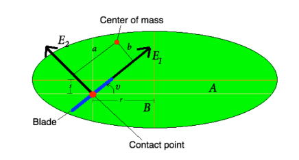
Figure 3: The elliptical sleigh. The blade makes an angle $\upsilon$ with the major axis of the ellipse and the contact point has coordinates $(r,s)$ with respect to the frame that is determined by the principal axes of the ellipse (in the diagram both $r$ and $s$ are negative).

For this geometry, starting from the formula (2.6) for the added inertia tensor given in section 2.1, one can show that

$$\tiny\mathbb{I}_{\mathcal{F}}=\rho\pi\left(\begin{array}[]{ccc}\begin{array}[]{c}\frac{(A^{2}-B^{2})^{2}}{4}+s^{2}(B^{2}\cos^{2}\upsilon+A^{2}\sin^{2}\upsilon)\\ +r^{2}(A^{2}\cos^{2}\upsilon+B^{2}\sin^{2}\upsilon)-rs(A^{2}-B^{2})\sin(2\upsilon)\end{array}&\begin{array}[]{c}s(B^{2}\cos^{2}\upsilon+A^{2}\sin^{2}\upsilon)\\ -\frac{1}{2}r(A^{2}-B^{2})\sin(2\upsilon)\end{array}&\begin{array}[]{c}-r(A^{2}\cos^{2}\upsilon+B^{2}\sin^{2}\upsilon)\\ +\frac{1}{2}s(A^{2}-B^{2})\sin(2\upsilon)\end{array}\\ &&\\ \begin{array}[]{c}s(B^{2}\cos^{2}\upsilon+A^{2}\sin^{2}\upsilon)\\ -\frac{1}{2}r(A^{2}-B^{2})\sin(2\upsilon)\end{array}&B^{2}\cos^{2}\upsilon+A^{2}\sin^{2}\upsilon&\frac{A^{2}-B^{2}}{2}\,\sin(2\upsilon)\\ &&\\ \begin{array}[]{c}-r(A^{2}\cos^{2}\upsilon+B^{2}\sin^{2}\upsilon)\\ +\frac{1}{2}s(A^{2}-B^{2})\sin(2\upsilon)\end{array}&\frac{A^{2}-B^{2}}{2}\,\sin(2\upsilon)&A^{2}\cos^{2}\upsilon+B^{2}\sin^{2}\upsilon\end{array}\right).$$ (3.12)

The total inertia tensor, $\mathbb{I}=\mathbb{I}_{\mathcal{B}}+\mathbb{I}_{\mathcal{F}}$, of the fluid-body system is then given by

$$\mathbb{I}=\left(\begin{array}[]{ccc}\begin{array}[]{c}\mathcal{I}+m(a^{2}+b^{2})\\ +\rho\pi[\frac{(A^{2}-B^{2})^{2}}{4}+s^{2}(B^{2}\cos^{2}\upsilon+A^{2}\sin^{2}\upsilon)\\ +r^{2}(A^{2}\cos^{2}\upsilon+B^{2}\sin^{2}\upsilon)-rs(A^{2}-B^{2})\sin(2\upsilon)]\end{array}&\begin{array}[]{c}-mb+\rho\pi[s(B^{2}\cos^{2}\upsilon+A^{2}\sin^{2}\upsilon)\\ -\frac{1}{2}r(A^{2}-B^{2})\sin(2\upsilon)]\end{array}&\begin{array}[]{c}ma+\rho\pi[-r(A^{2}\cos^{2}\upsilon+B^{2}\sin^{2}\upsilon)\\ +\frac{1}{2}s(A^{2}-B^{2})\sin(2\upsilon)]\end{array}\\ &&\\ \begin{array}[]{c}-mb+\rho\pi[s(B^{2}\cos^{2}\upsilon+A^{2}\sin^{2}\upsilon)\\ -\frac{1}{2}r(A^{2}-B^{2})\sin(2\upsilon)]\end{array}&m+\rho\pi[B^{2}\cos^{2}\upsilon+A^{2}\sin^{2}\upsilon]&\rho\pi\left[\frac{A^{2}-B^{2}}{2}\,\sin(2\upsilon)\right]\\ &&\\ \begin{array}[]{c}ma+\rho\pi[-r(A^{2}\cos^{2}\upsilon+B^{2}\sin^{2}\upsilon)\\ +\frac{1}{2}s(A^{2}-B^{2})\sin(2\upsilon)]\end{array}&\rho\pi\left[\frac{A^{2}-B^{2}}{2}\,\sin(2\upsilon)\right]&m+\rho\pi(A^{2}\cos^{2}\upsilon+B^{2}\sin^{2}\upsilon)\end{array}\right).$$

Notice that in the presence of the fluid, if $\upsilon\neq n\frac{\pi}{2},n\in\mathbb{Z}$, the coefficient $\mathbb{I}_{23}=\mathbb{I}_{32}$ is non-zero. This can never be the case if the sleigh is moving in vacuum as one can see from the expression given for $\mathbb{I}_{\mathcal{B}}$ in (2.3). The appearance of this non-zero term leads to interesting dynamics that, in the absence of circulation were studied in [11]. For the above geometry, the circulation constants $\alpha$ and $\beta$ defined by (2.10) are computed to be:

$$\alpha=\kappa(r\cos\upsilon+s\sin\upsilon),\qquad\beta=\kappa(-r\sin\upsilon+s\cos\upsilon).$$

Notice that, in the presence of circulation, the two constants, $\alpha$ and $\beta$, can vanish simultaneously only if $r=s=0$, that is, only if the contact point is at the center of the ellipse.

In the sequel we assume that the shape of the sleigh is arbitrary convex and that its center of mass does not necessarily coincide with the origin, which leads to the general total inertia tensor

$$\mathbb{I}=\left(\begin{array}[]{ccc}J&-L_{2}&L_{1}\\ -L_{2}&M&Z\\ L_{1}&Z&N\end{array}\right),$$

and with arbitrary circulation constants $\alpha,\,\beta$.

Detailed equations of motion.

The constraint written in terms of momenta is $v_{2}=\mathbb{I}^{-1}(k,p_{1},p_{2})^{T}=0$. Differentiating it and using (3.11), we find the multiplier

$$\lambda=-\frac{1}{({\mathbb{I}^{-1}})_{33}}\left(\mathbb{I}^{-1}\left(\begin{array}[]{c}v_{2}p_{1}-v_{1}p_{2}-\rho(\alpha v_{1}+\beta v_{2})\\ \omega p_{2}-\kappa\rho v_{2}+\rho\alpha\omega\\ -\omega p_{1}+\kappa\rho v_{1}+\rho\beta\omega)\end{array}\right)\right)_{3},$$

where

$$\mathbb{I}^{-1}=\frac{1}{\mbox{det}(\mathbb{I})}\left(\begin{array}[]{ccc}MN-Z^{2}&ZL_{1}+NL_{2}&-ZL_{2}-ML_{1}\\ ZL_{1}+NL_{2}&JN-L_{1}^{2}&-L_{1}L_{2}-JZ\\ -ZL_{2}-ML_{1}&-L_{1}L_{2}-JZ&JM-L_{2}^{2}\end{array}\right).$$

A long but straightforward calculation shows that, by expressing $\omega,v_{1}$ and $v_{2}$ in terms of $k,p_{1},p_{2}$, substituting into (3.11), and enforcing the constraint $v_{2}=0$, one obtains:

$$\begin{split}\dot{\omega}&=\frac{1}{D}\left(L_{1}\omega+Zv_{1}+\rho\alpha\right)\left(L_{2}\omega-Mv_{1}\right),\\ \dot{v}_{1}&=\frac{1}{D}\left(L_{1}\omega+Zv_{1}+\rho\alpha\right)\left(J\omega-L_{2}v_{1}\right),\end{split}$$ (3.13)

where we set $D=\operatorname{det}(\mathbb{I})({\mathbb{I}^{-1}})_{33}=MJ-L_{2}^{2}$. Note that $D>0$ since $\mathbb{I}$ and $\mathbb{I}^{-1}$ are positive definite. Note as well that if $\alpha=0$ we recover the system with zero circulation treated in [11] so from now on we assume $\alpha\neq 0$.

The full motion of the sleigh on the plane is determined by the reconstruction equations which, in our case with $v_{2}=0$, reduce to

$$\dot{\theta}=\omega,\qquad\dot{x}=v_{1}\cos\theta,\qquad\dot{y}=v_{1}\sin\theta.$$

The reduced energy integral has

$$H=\frac{1}{2}\left(J\omega^{2}+Mv_{1}^{2}-2L_{2}\omega v_{1}\right),$$

and its level sets are ellipses on the $(\omega\,v_{1})$-plane.

As seen from the equations, the straight line $\ell=\{L_{1}\omega+Zv_{1}+\rho\alpha=0\}$ consists of equilibrium points for the system. Each of these equilibria corresponds to a uniform circular motion on the plane along a circumference of radius $\left|\frac{v_{1}}{\omega}\right|$.

Notice that if $Z=L_{1}=0$ the line $\ell$ of equilibria disappears. In fact, it is shown in [12] that equations (3.13) possess an invariant measure only for this choice of the parameters. In this particular case we obtain simple harmonic motion on the reduced plane $\omega,v_{1}$.

For the sequel we will assume that $Z$ and $L_{1}$ are not both zero. We shall see that initial conditions with high energy yield asymptotic dynamics which is in agreement with our statement that there is no invariant measure in this case.

A level set of the energy will intersect once, twice or never the line of equilibra $\ell$ depending on the value of $H$. One can show that there are two intersections if $H>h_{0}$, only one intersection if $H=h_{0}$, and zero intersections if $H<h_{0}$, where

$$h_{0}=\frac{1}{2}(\rho\alpha)^{2}\frac{D}{E}$$

with $E=JZ^{2}+2ZL_{1}L_{2}+ML_{1}^{2}>0$.

Hence, the trajectories of (3.13) are contained in ellipses and they are of three types:

1. For small values of the energy, $0\leq H<h_{0}$, we have periodic motion on the ellipses.

2. For $H=h_{0}$ we have a homoclinic connection that separates periodic from asymptotic trajectories.

3. For $H>h_{0}$ we have heteroclinic connections between the asymptotically unstable and stable equilibria on $\ell$.

We introduce two other special energy values $h_{1},h_{2}\geq h_{0}$, for which the corresponding energy contour line intersects the equilibra line $\ell$ at the axes $\omega=0$ and $v_{1}=0$ respectively. Namely,

$$h_{1}=\frac{1}{2}\,\frac{(\rho\alpha)^{2}M}{Z^{2}},\qquad h_{2}=\frac{1}{2}\,\frac{(\rho\alpha)^{2}J}{L_{1}^{2}}.$$ (3.14)

The phase portrait is illustrated in Figure 4 (a).

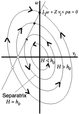
(a) Reduced phase portrait. The stable and unstable equilibra are represented by filled and empty dots, respectively.

(b) The 7 regions in the reduced phase space.

Figure 4: Reduced phase portrait and the 7 regions in phase space (assuming that $L_{1}>0$, $\alpha,Z<0$, and $h_{1}<h_{2}$).

Remark 1.

In fact, the reduced system (3.13) can be checked to be Hamiltonian with respect to the following Poisson bracket of functions of $\omega,v_{1}$

$$\{F_{1},F_{2}\}:=-\frac{1}{D}\left(L_{1}\omega+Zv_{1}+\rho\alpha\right)\left(\frac{\partial F_{1}}{\partial\omega}\frac{\partial F_{2}}{\partial v_{1}}-\frac{\partial F_{1}}{\partial v_{1}}\frac{\partial F_{2}}{\partial\omega}\right).$$

The invariant symplectic leaves consist of the semi-planes separated by the equilibria line $\ell$ and the zero-dimensional leaves formed by the points on $\ell$.

3.1 The motion of the sleigh on the plane: qualitative description

As for the reduced dynamics, the qualitative motion of the sleigh on the plane depends crucially on the energy value. We distinguish 7 regions on the reduced phase space as illustrated in Figure 4 (b). The regions are separated by the homoclinic orbit corresponding to the energy contour $H=h_{0}$, the two pairs of heteroclinic orbits corresponding to the energy contour lines $H=h_{1}$ and $H=h_{2}$, and the line of equilibra $\ell$. It is thus clear that the regions are invariant by the flow. We shall see that the qualitative motion of the sleigh is different in each region. The number of regions can change for special parameter values that make any of $h_{0},h_{1},h_{2}$ coincide. We shall discuss the behavior in the interior of the regions in the generic case where they are all different and under the assumption that $h_{1}<h_{2}$.

Motion in Region I.

For subcritical values of the energy, $0\leq H<h_{0}$, the reduced dynamics on $(v_{1},\omega)$ is periodic, but the motion on the sleigh is generally not periodic. Let $T$ be the (minimal) period of the reduced dynamics that depends on the energy value $H$ in a way that will be made precise in section 4. Under the shift $t\to t+T$ the coordinates of the sleigh undergo the increments

$$\Delta x=\int_{0}^{T}v_{1}(t)\cos\theta(t)\,dt,\qquad\Delta y=\int_{0}^{T}v_{1}(t)\sin\theta(t)\,dt,\qquad\Delta\theta=\int_{0}^{T}\omega(t)\,dt.$$ (3.15)

These quantities completely determine the type of motion of the sleigh.

Theorem 3.1.

Let $T$ be the period of a periodic solution to the reduced system (3.13) with $H<h_{0}$, and let ${\bf\Delta x}=(\Delta x,\Delta y)$ and $\Delta\theta$ be defined by (3.15). Then, the motion of the sleigh on the plane is

1. $T$-periodic if $\frac{\Delta\theta}{2\pi}\in\mathbb{Z}$ and ${\bf\Delta x}=0$.

2. Unbounded if $\frac{\Delta\theta}{2\pi}\in\mathbb{Z}$ and ${\bf\Delta x}\neq 0$.

3. Contained in a circle or an annulus if $\frac{\Delta\theta}{2\pi}\notin\mathbb{Z}$, where the motion

   1. is periodic of period $qT$ if $\frac{\Delta\theta}{2\pi}$ is a rational number written in terms of integers $p,q$ as $\frac{\Delta\theta}{2\pi}=\frac{p}{q}$ in irreducible form,

   2. fills up the annulus densely if $\frac{\Delta\theta}{2\pi}$ is irrational.

Moreover, the above types of the motion depend only on the energy value $H$. In particular, they are independent of the initial configuration of the sleigh.

Proof.

Assume without loss of generality that at $t=0$ the body and the space reference frames coincide. Then $\theta(0)=0$, and the element

$$S=\left(\begin{array}[]{ccc}\cos(\Delta\theta)&-\sin(\Delta\theta)&\Delta x\\ \sin(\Delta\theta)&\cos(\Delta\theta)&\Delta y\\ 0&0&1\end{array}\right)\in SE(2)$$

describes the shift in both reference frames after one period. Then the elements

$$g_{n}=\left(\begin{array}[]{ccc}\cos\theta(nT)&-\sin\theta(nT)&x(nT)\\ \sin\theta(nT)&\cos\theta(nT)&y(nT)\\ 0&0&1\end{array}\right)\in SE(2),\qquad n\in{\mathbb{Z}}$$

describing the subsequent positions of the sleigh in the space frame, are the right translations on $SE(2)$:

$$g_{n+1}=g_{n}S.$$

Following theorems of kinematics, each generic transformation of that kind is a rigid rotation about a fixed point $Q$ on the plane $(x,y)$ by the angle $\Delta\theta$. This happens when $\frac{\Delta\theta}{2\pi}\notin\mathbb{Z}$. Then the trajectory of the contact point lies inside of an annulus or a circle with the center $Q$. The trajectory is periodic iff $\frac{\Delta\theta}{2\pi}$ is a rational number, otherwise it fills the domain densely.

In the special case $\frac{\Delta\theta}{2\pi}\in\mathbb{Z}$ the transformation $g_{n}\to g_{n+1}$ is a parallel translation (if ${\bf\Delta x}\neq 0$), which is obviously unbounded, or is the identity (when ${\bf\Delta x}=0$), then the trajectory is periodic. This leads to the items of the theorem.

Finally note that the components of $S$ depend only on the energy value and not on the particular initial conditions. ∎

We mention that the matrix $S$ in the proof is the (right) monodromy matrix of the periodic linear system defined by the reconstruction equations. The global description of the invariant manifolds in the unreduced space, that generically are two-tori, can be studied with techniques similar to those developed in [8].

The types of motion indicated in items 2 and 3 of the above theorem are illustrated in Figure 5. The generic behavior of the sleigh corresponds to item 3 (b) (Figure 5 (c)).

Equation (4.19) in section 4 below gives the explicit dependence of $\Delta\theta$ on the energy.

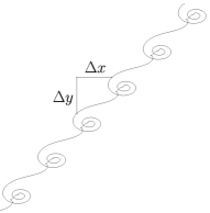
(a) Trajectory of the contact point with $\Delta\theta=-4\pi$, and $\Delta x,\Delta y\neq 0$ (unbounded motion).

(b) Trajectory of the contact point with $\Delta\theta=-\frac{11\pi}{7}$ (periodic motion in an annulus).

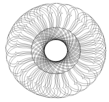
(c) Trajectory of the contact point with $\Delta\theta=-\frac{e\pi}{2}$ for a finite time (the trajectory fills the annulus densely).

Figure 5: Trajectory of the sleigh on the plane in region I ($H<h_{0}$) for different values of $\Delta\theta$.

Now notice that in the case $h\geq h_{0}$, the equilibria points $(\omega,v_{1})$ on the line $\ell=\{L_{1}\omega+Zv_{1}+\rho\alpha=0\}$ correspond to circular motion of the sleigh in the direction determined by the sign of $\omega$ (clockwise if $\omega>0$ and anti-clockwise if $\omega<0$). The circles describing by the contact point have radius $|v_{1}/\omega|$.

The exceptional cases when $\omega=0$ or $v_{1}=0$ respectively correspond to motion along a straight line or to a spinning motion of the sleigh about the contact point that remains fixed. These cases correspond respectively to the energy values $h_{1}$ and $h_{2}$. The motion of the sleigh on the plane when the energy attains the critical value $h_{0}$ will be discussed in section 4.

Motion in Region II.

The sleigh evolves asymptotically from one circular motion to another. The limit circles have different radii. Both of them are traversed counterclockwise (at the limit points in the region one has $\omega>0$). Moreover, the trajectory of the point of contact has two cusps corresponding to the two intersections with the axes $v_{1}=0$ on the Figure 4.

Motion in Region III.

The same behavior as in Region II, however, this time the trajectory has no cusps (since $v_{1}$ never vanishes).

Motion in Region IV.

The sleigh again evolves asymptotically from one circular motion to another. The limit circles have different radius and are are traversed in opposite directions. The trajectory of the contact point has two cusps corresponding to the two intersections with the axes $v_{1}=0$ on the plane $(v_{1},\omega)$.

Motion in Region V.

The same behavior as in Region IV, but the trajectory has no cusps since $v_{1}$ never vanishes.

Motion in Regions VI and VII.

The same behavior as in Region IV, however the trajectories have exactly one cusp corresponding to the intersection of the axis $v_{1}=0$.

(a) Region II.

(b) Region III.

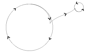
(c) Region IV.

Figure 6: Trajectories of the sleigh for initial conditions in regions II, III, and IV.

(a) Region V.

(b) Region VI.

(c) Region VII.

Figure 7: The trajectories for initial conditions in regions V, VI, and VII.

Thus we see that the qualitative behavior of the motion of the sleigh on the plane can be sensitive to initial conditions. This contrasts with the properties of other completely solvable classical nonholonomic systems like the Suslov problem or the hydrodynamic Chaplygin sleigh without circulation. For these systems one can obtain formulas for the parameters that determine the long term behavior of the dynamics, and such formulas are independent of the energy (see [11, 10]).

At the physical level, the motion of the sleigh can be understood as the interplay of two effects, the circulation of the fluid around the body, and the inertia of the body. For low energies ($H<h_{0}$) the dynamics are driven by the circulation and produce periodic motion in the reduced space. For high energies ($H>h_{0}$) the inertia of the body takes over and the asymptotic dynamics of the body on the plane resemble the motion of the hydrodynamic Chaplygin sleigh in the absence of circulation considered in [11].

We finally stress that all the above types of motion also appear in the classical Appel–Korteweg problem on the rolling of a non-vertical disc. Namely the trajectories of the contact point of the disc admit the same classification (see [1, 19, 9]).

4 Explicit solution of the reduced system in $se(2)^{*}$

We will only treat the case $L_{2}=0$ when the system (3.13) takes the form

$$\begin{split}\dot{\omega}&=\frac{1}{D}\left(L_{1}\omega+Zv_{1}+\rho\alpha\right)\left(-Mv_{1}\right),\\ \dot{v}_{1}&=\frac{1}{D}\left(L_{1}\omega+Zv_{1}+\rho\alpha\right)\left(J\omega\right),\end{split}$$ (4.16)

with $D=MJ$. The energy takes the diagonal form $H=\frac{1}{2}(J\omega^{2}+Mv_{1}^{2})$. The general case can be reduced to this one via an invertible linear change of variables as the following proposition shows.

Proposition 4.1.

There exists a $2\times 2$ rotation matrix $P\in SO(2)$ such that if $\omega$ and $v_{1}$ satisfy (3.13) then $(\tilde{\omega},\tilde{v}_{1})^{T}:=P(\omega,v_{1})^{T}$ satisfy (4.16) with coefficients $\tilde{L}_{1},\tilde{Z},\tilde{M},\tilde{J}$, where $\tilde{J},\tilde{M}>0$ satisfy $\tilde{M}\tilde{J}=D$, and $(\tilde{L}_{1},\tilde{Z})^{T}:=P(L_{1},Z)^{T}$.

Proof.

Define the restricted inertia tensor $\mathbb{I}_{c}$ by

$$\mathbb{I}_{c}:=\left(\begin{array}[]{cc}J&-L_{2}\\ -L_{2}&M\end{array}\right).$$

Since $\mathbb{I}_{c}$ is symmetric and positive definite, there exists $P\in{SO}(2)$ such that $P\,\mathbb{I}_{c}\,P^{T}$ is a diagonal matrix whose entries $\tilde{J},\tilde{M}>0$ are the eigenvalues of $\mathbb{I}_{c}$ and satisfy $\tilde{M}\tilde{J}=\mbox{det}\,\mathbb{I}_{c}=D$.

Equations (3.13) can be written in vector form as

$$\frac{d}{dt}\,\left(\begin{array}[]{c}\omega\\ v_{1}\end{array}\right)=\frac{1}{D}\left(\left\langle\left(\begin{array}[]{c}\omega\\ v_{1}\end{array}\right)\,,\,\left(\begin{array}[]{c}L_{1}\\ Z\end{array}\right)\right\rangle+\rho\alpha\right)\left(\begin{array}[]{cc}0&-1\\ 1&0\end{array}\right)\,\mathbb{I}_{c}\,\left(\begin{array}[]{c}\omega\\ v_{1}\end{array}\right),$$

where $\langle\cdot,\cdot\rangle$ denotes the usual inner product in $\mathbb{R}^{2}$. Defining $(\tilde{\omega},\tilde{v}_{1})^{T}:=P(\omega,v_{1})^{T}$, the above equations are equivalent to

$$\frac{d}{dt}\,\left(\begin{array}[]{c}\tilde{\omega}\\ \tilde{v}_{1}\end{array}\right)=\frac{1}{D}\left(\left\langle\left(\begin{array}[]{c}\tilde{\omega}\\ \tilde{v}_{1}\end{array}\right)\,,\,P\,\left(\begin{array}[]{c}L_{1}\\ Z\end{array}\right)\right\rangle+\rho\alpha\right)\,P\,\left(\begin{array}[]{cc}0&-1\\ 1&0\end{array}\right)\,\mathbb{I}_{c}\,P^{T}\,\left(\begin{array}[]{c}\tilde{\omega}\\ \tilde{v}_{1}\end{array}\right).$$

The result now follows by noticing that

$$P\,\left(\begin{array}[]{cc}0&-1\\ 1&0\end{array}\right)\,\mathbb{I}_{c}\,P^{T}=\left(\begin{array}[]{cc}0&-1\\ 1&0\end{array}\right)\,P\,\mathbb{I}_{c}\,P^{T}=\left(\begin{array}[]{cc}0&-1\\ 1&0\end{array}\right)\left(\begin{array}[]{cc}\tilde{J}&0\\ 0&\tilde{M}\end{array}\right)$$

where we have used that $P\in SO(2)$ in the first equality. ∎

The solution of the system (4.16) can be obtained by parameterizing level set $H=h$ of the energy function $H=\frac{1}{2}(J\omega^{2}+Mv_{1}^{2})$ as

$$\omega(t)=\sqrt{\frac{2h}{J}}\left(\frac{2f(t)}{f(t)^{2}+1}\right),\qquad v_{1}(t)=\pm\sqrt{\frac{2h}{M}}\left(\frac{f(t)^{2}-1}{f(t)^{2}+1}\right).$$

Substitution into (4.16) gives a separable equation for $f(t)$ of the form

$$\dot{f}(t)=Af(t)^{2}+2Bf(t)+C,$$ (4.17)

where the coefficients $A,B,C,$ depend on the entries of the inertia tensor $\mathbb{I}$, on $\rho\alpha$, and also on the energy value $h$. The form of the solutions for the above equation depends on the sign of the discriminant $\Delta:=B^{2}-AC$. A long but straightforward calculation shows that

$$\Delta=\frac{1}{2}\left(\frac{E}{D^{2}}\right)(h-h_{0}),$$

and hence $\mbox{sign}(\Delta)=\mbox{sign}(h-h_{0})$. Therefore the form of the solution varies depending on whether the energy $h$ is higher than, smaller than or equal to the critical energy level $h_{0}$. We will now give the explicit formulae for $\omega$ and $v_{1}$ in these three cases. To write our formulas in a compact and unified manner we introduce the coefficients:

$$\begin{split}\gamma&:=\sqrt{|\Delta|}=\frac{\sqrt{E}}{\sqrt{2}D}\sqrt{|h-h_{0}|},\qquad K_{1}:=\frac{\sqrt{E}}{Z\sqrt{J}}\left(\frac{\sqrt{|h-h_{0}|}}{\sqrt{h}+\sqrt{h_{1}}}\right),\\ K_{2}&:=-\mbox{sign}(\alpha Z)\frac{L_{1}\sqrt{M}}{Z\sqrt{J}}\left(\frac{\sqrt{h}}{\sqrt{h_{1}}+\sqrt{h}}\right),\qquad K_{3}:=-\frac{\sqrt{2}M\sqrt{J}}{Z}\left(\frac{1}{\sqrt{h_{0}}+\sqrt{h_{1}}}\right),\end{split}$$ (4.18)

where $h_{1}$ is given by (3.14), and we assume that the constants $L_{1},Z$, are non-zero. Notice that $\gamma,K_{1},$ and $K_{2}$ depend on the energy value $h$.

The solution for $0<h<h_{0}$.

In this case the discriminant $\Delta<0$ and $f(t)=\frac{1}{A}(\gamma\tan(\gamma t)-B)$ is a solution of (4.17). After some algebra this gives the following solution of (4.16):

$$\begin{split}\omega(t)&=2\sqrt{\frac{2h}{J}}\left(\frac{K_{2}\cos^{2}(\gamma t)+K_{1}\sin(\gamma t)\cos(\gamma t)}{(1+K_{2}^{2})\cos^{2}(\gamma t)+2K_{1}K_{2}\sin(\gamma t)\cos(\gamma t)+K_{1}^{2}\sin^{2}(\gamma t)}\right),\\ v_{1}(t)&=\mbox{sign}(\alpha Z)\sqrt{\frac{2h}{M}}\left(\frac{(K^{2}_{2}-1)\cos^{2}(\gamma t)+2K_{1}K_{2}\sin(\gamma t)\cos(\gamma t)+K_{1}^{2}\sin^{2}(\gamma t)}{(1+K_{2}^{2})\cos^{2}(\gamma t)+2K_{1}K_{2}\sin(\gamma t)\cos(\gamma t)+K_{1}^{2}\sin^{2}(\gamma t)}\right).\end{split}$$

We immediately obtain the following formula for the period $T$ of the solutions:

$$T=\frac{\pi}{\gamma}=\frac{\sqrt{2}\pi D}{\sqrt{E}\sqrt{h_{0}-h}}.$$

Notice that $T\rightarrow\infty$ as $h\rightarrow h_{0}$ from the left as expected.

We can also obtain a closed expression for the increment $\Delta\theta=\int_{0}^{T}\omega(t)\,dt$. For this matter we note that a primitive of $\omega(t)$ is given by (see e.g. [13]):

$$\theta(t)=\frac{2}{\gamma}\sqrt{\frac{2h}{J}}\,\left(\frac{\theta_{1}(t)+\theta_{2}(t)+\theta_{3}(t)}{4K_{1}^{2}K_{2}^{2}+(1+K_{2}^{2}-K_{1}^{2})^{2}}\right),$$

with

$$\begin{split}\theta_{1}(t)&=K_{2}(1+K_{1}^{2}+K_{2}^{2})\gamma t,\\ \theta_{2}(t)&=\frac{K_{1}}{2}(K_{1}^{2}+K_{2}^{2}-1)\,\ln((1+K_{2}^{2})\cos^{2}(\gamma t)+2K_{1}K_{2}\sin(\gamma t)\cos(\gamma t)+K_{1}^{2}\sin^{2}(\gamma t)),\\ \theta_{3}(t)&=-2K_{1}K_{2}\arctan(K_{1}\tan(\gamma t)+K_{2}).\end{split}$$

Therefore, taking into account the change of branch in the expression for $\theta_{3}(t)$, we find that, under the above assumption $L_{2}=0$,

$$\Delta\theta=\theta(\pi/\gamma)-\theta(0)=\frac{2\pi}{\gamma}\sqrt{\frac{2h}{J}}\,\left(\frac{K_{2}(1+K_{1}^{2}+K_{2}^{2})+2K_{1}K_{2}}{4K_{1}^{2}K_{2}^{2}+(1+K_{2}^{2}-K_{1}^{2})^{2}}\right).$$ (4.19)

(In the general case $L_{2}\neq 0$ due to Proposition 4.1, $\Delta\theta$ will be a linear combination of (4.19)) and of the integral $\int_{0}^{T}v_{1}(t)\,dt$.)

In particular notice that $\Delta\theta=O((h_{0}-h)^{-1/2})$ as $h\rightarrow h_{0}$ from the left. This implies that the behavior of the sleigh on the plane is extremely sensitive to the energy values that are slightly smaller than $h_{0}$. Namely, we have

Proposition 4.2.

For any $\delta>0$ there exists a strictly increasing sequence of energy values $\{h^{(p)}_{k}\}_{k\in\mathbb{N}}$ satisfying $h_{0}-\delta<h^{(p)}_{k}<h_{0}$, for which the motion of the contact point in the plane is periodic. Similarly, there exists an increasing sequence of energy values $\{h^{(u)}_{k}\}_{k\in\mathbb{N}}$ (respectively, $\{h^{(q)}_{k}\}_{k\in\mathbb{N}}$) satisfying
$h_{0}-\delta<h^{(u)}_{k}<h_{0}$ (respectively, $h_{0}-\delta<h^{(q)}_{k}<h_{0}$), such that the motion of the sleigh is unbounded (respectively, quasiperiodic).

The proof follows from the results of Theorem 3.1 and the fact that $|\Delta\theta|\to\infty$ as $h\to h_{0}$ from the left.

The solution for $h=h_{0}$.

In this case the discriminant $\Delta=0$, and (4.17) has the solution
$f(t)=-\frac{1}{A}(\frac{1}{t}+B)$. After some algebra this gives the following solution of (4.16):

$$\begin{split}\omega(t)&=2\sqrt{\frac{2h_{0}}{J}}\,\frac{K_{3}t+K_{2}t^{2}}{(1+K_{2}^{2})t^{2}+2K_{3}K_{2}t+K_{3}^{2}}\,,\\ v_{1}(t)&=\mbox{sign}(\alpha Z)\sqrt{\frac{2h_{0}}{M}}\,\frac{(K^{2}_{2}-1)t^{2}+2K_{3}K_{2}t+K_{3}^{2}}{(1+K_{2}^{2})t^{2}+2K_{3}K_{2}t+K_{3}^{2}}\,,\end{split}$$

where it is understood that $h=h_{0}$ in the expression for $K_{2}$.

To analyze the trajectory of the contact point of the sleigh, consider the particular solution $\omega(t-t_{0}),\,v_{1}(t-t_{0})$ with $t_{0}=-\frac{K_{2}K_{3}}{1+K_{2}^{2}}$. In order to keep the notation as simple as possible, we will also denote this solution by $\omega(t),\,v_{1}(t)$. We have

$$\begin{split}\omega(t)&=2\sqrt{\frac{2h_{0}}{J}}\left(\frac{C_{1}^{2}K_{2}t^{2}-K_{3}C_{1}C_{2}t-K_{2}K_{3}^{2}}{C_{1}(C_{1}^{2}t^{2}+K_{3}^{2})}\right),\\ v_{1}(t)&=\mbox{sign}(\alpha Z)\sqrt{\frac{2h_{0}}{M}}\left(\frac{C_{1}^{2}C_{2}t^{2}+4K_{3}K_{2}C_{1}t-K_{3}^{2}C_{2}}{C_{1}(C_{1}^{2}t^{2}+K_{3}^{2})}\right),\end{split}$$

where $C_{1}=1+K_{2}^{2}$ and $C_{2}=K_{2}^{2}-1$.

Notice that

$$\lim\limits_{t\to\pm\infty}\frac{v_{1}}{\omega}=\frac{1}{2}\mbox{sign}(\alpha Z)\sqrt{\frac{J}{M}}\frac{C_{2}}{K_{2}}:=R,$$

hence the limit motions of the sleigh are along circles of the same radius $|R|$. Moreover, the circles are traversed in the same direction as both $\omega(t)$ and $v_{1}(t)$ have the same limits as $t\to\pm\infty$.

Proposition 4.3.

The motion of the contact point in the plane in the case $h=h_{0}$ is bounded.

Proof.

It is sufficient to show that the distance between the centers of the limit circumferences is finite. The centers coincide with limit positions of the point $C$ of the sleigh with body coordinates $(0,R)$. Indeed, the components of the velocity of this point are given by

$$\dot{x}_{C}=V_{C}(t)\cos(\theta(t)),\qquad\dot{y}_{C}=V_{C}(t)\sin(\theta(t)),$$

where

$$V_{C}(t)=v_{1}(t)-R\omega(t)=\mbox{sign}(\alpha Z)\sqrt{\frac{2h_{0}}{M}}\frac{K_{3}(4K_{2}^{2}+C_{2}^{2})t}{K_{2}(C_{1}^{2}t^{2}+K_{3}^{2})},$$

that goes to zero as $t\to\pm\infty$. Therefore, the vector that connects the two centers has the components

$$\Delta x_{C}=\int_{-\infty}^{\infty}V_{C}(t)\cos\theta(t)\,dt,\qquad\Delta y_{C}=\int_{-\infty}^{\infty}V_{C}(t)\sin\theta(t)\,dt,$$

where $\theta(t)=\theta_{1}(t)+\theta_{2}(t)+\theta_{3}(t)$ with

$$\begin{split}\theta_{1}(t)&=2\sqrt{\frac{2h_{0}}{J}}\frac{K_{2}t}{C_{1}},\qquad\theta_{2}(t)=-\sqrt{\frac{2h_{0}}{J}}\frac{K_{3}C_{2}}{C_{1}^{2}}\ln(C_{1}^{2}t^{2}+K_{3}^{2})+\theta_{0},\\ \theta_{3}(t)&=-4\sqrt{\frac{2h_{0}}{J}}\frac{K_{3}K_{2}}{C_{1}^{2}}\arctan\left(\frac{C_{1}t}{K_{3}}\right),\end{split}$$

$\theta_{0}$ being an integration constant. Notice that $\theta_{1},\theta_{3}$ and $V_{C}$ are odd functions of $t$ whereas $\theta_{2}$ is even. Therefore, using basic trigonometric identities, we get:

$$\Delta x_{C}=-\int_{-\infty}^{\infty}V_{C}\sin(\theta_{1})\sin(\theta_{2})\cos(\theta_{3})\,dt-\int_{-\infty}^{\infty}V_{C}\cos(\theta_{1})\sin(\theta_{2})\sin(\theta_{3})\,dt.$$

The above integrals can be shown to converge using integration by parts. For example, using that $\sin(\theta_{1})=\frac{d}{dt}(-C_{3}\cos(\theta_{1}))$ for a certain constant $C_{3}$, the first integral rereads

$$\int_{-\infty}^{\infty}V_{C}\sin(\theta_{1})\sin(\theta_{2})\cos(\theta_{3})\,dt=-C_{3}\cos(\theta_{1})V_{C}\sin(\theta_{2})\cos(\theta_{3})\big{|}_{-\infty}^{\infty}+C_{3}\int_{-\infty}^{\infty}\cos(\theta_{1})k(t)\,dt,$$

where $k(t)=\frac{d}{dt}(V_{C}\sin(\theta_{2})\cos(\theta_{3}))$. It is seen that the two terms on the right are finite. Namely, the limits of the boundary terms are zero since $V_{C}\to 0$ as $t\to\pm\infty$. Next, the integral is absolutely convergent since $|k(t)|$ can be dominated by a function that decays as $1/t^{2}$ for large $|t|$.

The proof that $\Delta y_{C}$ is finite is analogous. ∎

The solution for $h>h_{0}$.

In this case the discriminant $\Delta>0$ and two solutions of (4.17) should be considered. These are $f_{1}(t)=\frac{1}{C}(-\gamma\tanh(\gamma t)-B)$ and $f_{2}(t)=\frac{1}{C}(-\gamma\coth(\gamma t)-B)$, and correspond to the two heteroclinic orbits that, together with the equilibra, make up the energy contour.

Starting out with $f_{1}(t)$ we find the solution to (4.16)

$$\begin{split}\omega(t)&=2\sqrt{\frac{2h}{J}}\left(\frac{K_{2}\cosh^{2}(\gamma t)-K_{1}\sinh(\gamma t)\cosh(\gamma t)}{(1+K_{2}^{2})\cosh^{2}(\gamma t)-2K_{1}K_{2}\sinh(\gamma t)\cosh(\gamma t)+K_{1}^{2}\sinh^{2}(\gamma t)}\right),\\ v_{1}(t)&=\mbox{sign}(\alpha Z)\sqrt{\frac{2h}{M}}\left(\frac{(K^{2}_{2}-1)\cosh^{2}(\gamma t)-2K_{1}K_{2}\sinh(\gamma t)\cosh(\gamma t)+K_{1}^{2}\sinh^{2}(\gamma t)}{(1+K_{2}^{2})\cosh^{2}(\gamma t)-2K_{1}K_{2}\sinh(\gamma t)\cosh(\gamma t)+K_{1}^{2}\sinh^{2}(\gamma t)}\right),\end{split}$$ (4.20)

that is contained in the semi-plane $L_{1}\omega+Zv_{1}+\rho\alpha>0.$

Whereas considering $f_{2}(t)$ one finds the solution to (4.16)

$$\begin{split}\omega(t)&=2\sqrt{\frac{2h}{J}}\left(\frac{K_{2}\sinh^{2}(\gamma t)-K_{1}\sinh(\gamma t)\cosh(\gamma t)}{(1+K_{2}^{2})\sinh^{2}(\gamma t)-2K_{1}K_{2}\sinh(\gamma t)\cosh(\gamma t)+K_{1}^{2}\cosh^{2}(\gamma t)}\right),\\ v_{1}(t)&=\mbox{sign}(\alpha Z)\sqrt{\frac{2h}{M}}\left(\frac{(K^{2}_{2}-1)\sinh^{2}(\gamma t)-2K_{1}K_{2}\sinh(\gamma t)\cosh(\gamma t)+K_{1}^{2}\cosh^{2}(\gamma t)}{(1+K_{2}^{2})\sinh^{2}(\gamma t)-2K_{1}K_{2}\sinh(\gamma t)\cosh(\gamma t)+K_{1}^{2}\cosh^{2}(\gamma t)}\right),\end{split}$$

that is contained in the semi-plane $L_{1}\omega+Zv_{1}+\rho\alpha<0.$

For the sequel, we only consider the branch of the solution corresponding to the expressions for $\omega(t)$ and $v_{1}(t)$ given by (4.20).

Integrating $\omega(t)$ and denoting $\kappa=2\sqrt{2h/J}$, we get

$$\theta(t) =\int\omega\,dt=\theta_{1}+\theta_{2}+\theta_{3},$$

$$\theta_{1} =\kappa\frac{K_{1}+K_{2}}{(K_{1}+K_{2})^{2}+1}\,t,$$

$$\theta_{2} =\kappa\frac{K_{1}}{2\gamma}\frac{K_{2}^{2}-K_{1}^{2}-1}{[(K_{1}+K_{2})^{2}+1]\cdot[(K_{1}-K_{2})^{2}+1]}$$

$$\qquad\cdot\ln\left([(K_{1}-K_{2})^{2}+1]e^{4\gamma t}+[2(K_{2}^{2}-K_{1}^{2}+1)]e^{2\gamma t}+[(K_{1}+K_{2})^{2}+1]\right),$$

$$\theta_{3} =\kappa\frac{2K_{1}K_{2}}{\gamma[(K_{1}+K_{2})^{2}+1]\cdot[(K_{1}-K_{2})^{2}+1]}\arctan\left(\frac{1}{2K_{1}}[(K_{1}-K_{2})^{2}+1]e^{2\gamma t}+\frac{1}{2K_{1}}[K_{2}^{2}-K_{1}^{2}+1]\right).$$

We will assume that $\mbox{sign}(\alpha Z)=1$ in the expression for $v_{1}$. Note that the radii of the limit circles are different:

$$r_{\pm}=\lim_{t\to\pm\infty}\frac{v_{1}}{\omega}=\frac{1}{2}\sqrt{\frac{J}{M}}\frac{(K_{2}\mp K_{1})^{2}-1}{K_{2}\mp K_{1}}.$$

Then, to evaluate the distance between their centers, introduce the “floating radius”

$$\rho(t)=\frac{r_{+}e^{\gamma t}+r_{-}e^{-\gamma t}}{e^{\gamma t}+e^{-\gamma t}},\text{so that}\quad\rho(\pm\infty)=r_{\pm},$$

and the floating point of the sleigh whose coordinates in the body fixed frame are $(0,\rho(t))$. The limit positions of this point coincide with the centers of the limit circumferences. The components of the velocity of the point are

$$\dot{x}_{\rho}=V_{\rho}(t)\cos\theta(t),\qquad\dot{y}_{\rho}=V_{\rho}(t)\sin\theta(t),$$

where

$$V_{\rho}(t)=v_{1}(t)-\rho(t)\omega(t)=\sqrt{\frac{2h}{M}}\frac{4K_{1}^{2}}{K_{2}^{2}-K_{1}^{2}}\cdot\frac{1}{[(K_{1}-K_{2})^{2}+1]e^{2\gamma t}+2[K_{2}^{2}-K_{1}^{2}-1]+[(K_{1}+K_{2})^{2}+1]e^{-2\gamma t}},$$

Now introduce the new variable

$$z=\frac{1}{2K_{1}}[(K_{1}-K_{2})^{2}+1]e^{2\gamma t},$$

and the constant

$$k:=K_{2}^{2}-K_{1}^{2}+1=\frac{Eh_{0}+JZ^{2}(2\sqrt{hh_{1}}+h_{1})}{(\sqrt{h_{1}}+\sqrt{h})^{2}}.$$ (4.21)

Then

$$e^{2\gamma t}=\frac{2K_{1}z}{(K_{1}-K_{2})^{2}+1},$$

$$dz=\frac{\gamma}{K_{1}}[(K_{1}-K_{2})^{2}+1]e^{2\gamma t}\,dt=2\gamma z\,dt,$$ (4.22)

$$z^{2}+\frac{k}{K_{1}}z+\frac{k^{2}}{4K_{1}^{2}}+1=\frac{(K_{1}-K_{2})^{2}+1}{4K_{1}^{2}}\left([(K_{1}-K_{2})^{2}+1]e^{4\gamma t}+2(K_{2}^{2}-K_{1}^{2}+1)e^{2\gamma t}+(K_{1}+K_{2})^{2}+1\right).$$

and, therefore,

$$\theta_{1} =\kappa\frac{K_{1}+K_{2}}{(K_{1}+K_{2})^{2}+1}\frac{1}{2\gamma}\ln\left(\frac{2K_{1}z}{(K_{1}-K_{2})^{2}+1}\right),$$

$$\theta_{2} =\kappa\frac{K_{1}}{2\gamma}\frac{K_{2}^{2}-K_{1}^{2}-1}{[(K_{1}+K_{2})^{2}+1]\cdot[(K_{1}-K_{2})^{2}+1]}\ln\left(z^{2}+\frac{k}{K_{1}}z+\frac{k^{2}}{4K_{1}^{2}}+1\right)\quad\text{(up to an additive constant)},$$

$$\theta_{3} =\kappa\frac{2K_{1}K_{2}}{\gamma[(K_{1}+K_{2})^{2}+1]\cdot[(K_{1}-K_{2})^{2}+1]}\arctan\left(z+\frac{k}{2K_{1}}\right),$$

$$V_{\rho} =\sqrt{\frac{2h}{M}}\,\frac{[(K_{1}-K_{2})^{2}+1]}{K_{2}^{2}-K_{1}^{2}}\,\frac{1}{z^{2}+\frac{k}{K_{1}}z+\frac{k^{2}}{4K_{1}^{2}}+1}\,e^{2\gamma t}=\sqrt{\frac{2h}{M}}\frac{1}{z^{2}+\frac{k}{K_{1}}z+\frac{k^{2}}{4K_{1}^{2}}+1}\frac{2K_{1}z}{K_{2}^{2}-K_{1}^{2}}\,.$$

The components of the vector of the distance between the centers of the limit circles are

$$\Delta x_{\rho}=\int_{-\infty}^{\infty}V_{\rho}\cos\theta(t)\,dt,\quad\Delta y_{\rho}=\int_{-\infty}^{\infty}V_{\rho}\sin\theta(t)\,dt$$

Then, in view of (4.22),

$$\Delta x_{\rho} =\sqrt{\frac{2h}{M}}\frac{2K_{1}}{K_{2}^{2}-K_{1}^{2}}\,\int_{-\infty}^{\infty}\frac{z}{z^{2}+\frac{K_{3}}{K_{1}}z+\frac{K_{3}^{2}}{4K_{1}^{2}}+1}\cos\theta(t)\,dt$$

$$=\sqrt{\frac{2h}{M}}\frac{K_{1}}{\gamma(K_{2}^{2}-K_{1}^{2})}\,\int_{0}^{\infty}\frac{\cos\theta}{z^{2}+\frac{K_{3}}{K_{1}}z+\frac{K_{3}^{2}}{4K_{1}^{2}}+1}dz,$$

and similarly for $\Delta y_{\rho}$.

Under the next substitution $z=\tan u$ the above integrals yield

$$\Delta x_{C}\pm i\Delta y_{C}=\frac{\sqrt{2h/M}\,K_{1}}{\gamma(K_{2}^{2}-K_{1}^{2})}a_{0}^{\pm ia_{1}}\int_{0}^{\pi/2}\frac{(\sin u)^{\pm ia_{1}}(\cos u)^{\mp i(a_{1}+2a_{2})}\exp\left(\pm ia_{3}\arctan\left(\tan u+\frac{k}{2K_{1}}\right)\right)}{\left(1+\frac{k}{2K_{1}}\sin(2u)+\frac{k^{2}}{4K_{1}^{2}}\cos^{2}u\right)^{1\mp ia_{2}}}\,du,$$ (4.23)

$$a_{0}=\frac{2K_{1}}{(K_{1}-K_{2})^{2}+1},\quad a_{1}=\frac{\kappa(K_{1}+K_{2})}{2\gamma((K_{1}+K_{2})^{2}+1)},$$

$$a_{2}=\frac{\kappa K_{1}(K_{2}^{2}-K_{1}^{2}-1)}{2((K_{1}+K_{2})^{2}+1)((K_{1}-K_{2})^{2}+1)},\quad a_{3}=\frac{2\kappa K_{1}K_{2}}{\gamma((K_{1}+K_{2})^{2}+1)((K_{1}-K_{2})^{2}+1)}.$$

The latter integrals represent a generalization of the classical Beta-function (see, e.g., [13]). Their product gives the square of the distance between the centers.

Remark.

We could not calculate the above integrals explicitly. Note, however, that in the limit $h\to\infty$, when the energy prevails over the circulation effect, due to (4.18) and (4.21), the integrals (4.23) reduce to

$$\Delta x_{C}\pm i\Delta y_{C}=-\frac{2\sqrt{D}}{Z}c_{0}^{\mp i\zeta}\int_{0}^{\pi/2}(\sin u)^{\mp i\zeta}(\cos u)^{\mp i\zeta}\left(\cos(2c_{1}\,u)\mp i\sin(2c_{1}\,u)\right)\,du.$$

$$\zeta=\frac{DZ}{E},\qquad c_{1}=\frac{\sqrt{D}ML_{1}}{E},\qquad c_{0}=\frac{Z\sqrt{D}}{\sqrt{EM}+L_{1}M}.$$

Note that the same reduction holds in case of zero circulation ($h_{0}=h_{1}=0$ in (4.21) implies $k=0$), which was studied in [11]. As was shown there, the product of the above integrals gives the square of the distance between the centers in the following closed form

$$(\Delta x_{C})^{2}+(\Delta y_{C})^{2}=\frac{2\pi D}{Z^{2}}\left(\frac{\zeta}{c_{1}^{2}+\zeta^{2}}\right)\left(\frac{\cosh(\zeta\pi)-\cos(c_{1}\pi)}{\sinh(\zeta\pi)}\right).$$

Conclusions and further work

We presented one of the first examples of nonholonomic hydrodynamical system, which is related to the design of underwater vehicles. The nonholonomic constraint can be interpreted as a first approximation model for a fin. From the mathematical point of view, our example is remarkable since both asymptotic and periodic dynamics coexist in the reduced phase space. It has been observed that the value of the energy is a crucial parameter in the qualitative behavior of the body on the plane. To our knowledge, this type of phenomenon is quite rare in nonholonomic dynamics. (A similar behavior occurs in the classical Appel–Korteweg problem on the rolling disc [1, 9].)

For the future, we intend to study the motion of the hydrodynamic Chaplygin sleigh coupled to point vortices in the fluid [21]. The equations of motion for interacting point vortices and rigid bodies (without nonholonomic constraints) were recently derived in [26, 2] and since then there have been significant efforts towards discerning integrability and chaoticity [22, 24] and towards uncovering the underlying geometry of these models [28]. We plan to couple the nonholonomic Chaplygin sleigh with one or several point vortices in the flow, taking these models as our next starting point.

Acknowledgments

We thank the GMC (Geometry, Mechanics and Control Network, project MTM2009-08166-E, Spain) for facilitating our collaboration during the events that it organizes.

Yu.N.F’s contribution was partially supported by the project MICINN MTM2009-06973.

We are also thankful to Hassan Aref, Francesco Fassò, Andrea Giacobbe, and Paul Newton for useful and interesting discussions, and to Maria Przybylska who helped us to integrate the reduced system (4.16).

JV is a postdoc at the Department of Mathematics of UC San Diego, partially supported by NSF CAREER award DMS-1010687 and NSF FRG grant DMS-1065972, and by the irses project geomech (nr. 246981) within the 7th European Community Framework Programme, and is on leave from a Postdoctoral Fellowship of the Research Foundation–Flanders (FWO-Vlaanderen). LGN acknowledges the hospitality of the Department de Matemática Aplicada I, and IV, at UPC Barcelona for his recent stay there.

References

- [1] Appell, P. Traite de mechanique rationelle, Vol. 2, Gauthier–Villars, Paris, 1953.
- [2] Borisov A.V., Mamaev I.S., and Ramodanov S.M., Motion of a circular cylinder and point vortices in a perfect fluid. Reg. and Chaot. Dyn., 8 (2003), no. 4, 449–462.
- [3] Borisov A.V., and Mamaev I.S., On the motion of a heavy rigid body in an ideal fluid with circulation. Chaos 16 (2006), no. 1, 013118.
- [4] T. Chambrion and A. Munnier. On the locomotion and control of a self-propelled shape-changing body in a fluid. To be published in J. Nonlin. Sci., 2011.
- [5] T. Chambrion and M. Sigalotti. Tracking control for an ellipsoidal submarine driven by Kirchhoff’s laws. IEEE Trans. Automat. Control, 53(1):339–349, 2008.
- [6] S. A. Chaplygin. On the effect of a plane-parallel air flow on a cylindrical wing moving in it. The Selected Works on Wing Theory of Sergei A. Chaplygin., pages 42–72, 1956. Translated from the 1933 Russian original by M. A. Garbell.
- [7] Chaplygin, S. A., On the Theory of Motion of Nonholonomic Systems. The theorem of the Reducing Multiplier. Math. Sbornik XXVIII, (1911) 303–314, (in Russian).
- [8] Fassò, F., and Giacobbe, A., Geometry of invariant tori of certain integrable systems with symmetry and an application to a nonholonomic system. SIGMA Symmetry Integrability Geom. Methods Appl. 3 (2007), 051, 12 pages.
- [9] Fedorov Yu. N., Rolling of a disc over an absolutely rough surface Izv. Akad. Nauk SSSR, Mekh.Tverd.Tela (Russian) 54 (1987), 67–75, Eng. transl. in Mechanics of Solids 22 (1988), No.4, 65–73.
- [10] Fedorov Yu. N., Maciejewski, A. J. and Przybylska, M., The Poisson equations in the nonholonomic Suslov problem: integrability, meromorphic and hypergeometric solutions. Nonlinearity, 22 (2009), no. 9, 2231-2259.
- [11] Fedorov Y. N. and García-Naranjo, L. C., The hydrodynamic Chaplygin sleigh. J. Phys. A: Math. Theor. 43 (2010) 434013 (18pp).
- [12] García-Naranjo, L. C. and Vankerschaver, J., Nonholonomic LL systems on central extensions and the hydrodynamic Chaplygin sleigh with circulation, arXiv:1109.3210v1
- [13] Gradshteyn, I. S., Ryzhik, I. M., Tables of series, products and integrals. 7th ed. San Diego, Academic Press 2007.
- [14] Kanso E., Marsden J. E., Rowley, C. W., and Melli-Huber J. B., Locomotion of Articulated Bodies in a Perfect Fluid J. Nonlinear Sci., 15 (2005), 255–289.
- [15] S. Kelly and R. Hukkeri. Mechanics, dynamics, and control of a single-input aquatic vehicle with variable coefficient of lift. IEEE Transactions on Robotics, 22(6):1254 –1264, dec. 2006.
- [16] G. R. Kirchhoff. Vorlesunger über Mathematische Physik, Band I, Mechanik. Teubner, Leipzig, 1877.
- [17] Lamb, H., Hydrodynamics. 6 ed. Dover, NY, 1932.
- [18] N. E. Leonard. Stability of a bottom-heavy underwater vehicle. Automatica J. IFAC, 33(3):331–346, 1997.
- [19] Levi-Civita, T., Amaldi, U. Lezioni di meccanica razionale. Vol. 2. Dinamica dei sistemi con un numero finito di gradi di liberta. (Italian) Nuova ed. N. Zanichelli, Bologna, 1951, 1952
- [20] L. Milne-Thomson. Theoretical hydrodynamics. London: MacMillan and Co. Ltd., fifth edition, revised and enlarged edition, 1968.
- [21] P. K. Newton. The -vortex problem. Analytical techniques, volume 145 of Applied Mathematical Sciences. Springer-Verlag, New York, 2001.
- [22] Ramodanov, S.M. Motion of a circular cylinder and a vortex in an ideal fluid. Reg. and Chaot. Dyn., 6 (2000), no. 1, 33–38.
- [23] Rand, R. H. and Ramani D.V. Relaxing Nonholonomic Constraints. In: Proceedings of the First International Symposium on Impact and Friction of Solids, Structures, and Intelligent Machines, (A. Guran, ed.), World Scientific, Singapore, 2000, 113-116
- [24] J. Roenby and H. Aref. Chaos in body-vortex interactions. Proc. R. Soc. Lond. Ser. A Math. Phys. Eng. Sci., 466(2119):1871–1891, 2010.
- [25] P. G. Saffman. Vortex dynamics. Cambridge Monographs on Mechanics and Applied Mathematics. Cambridge University Press, New York, 1992.
- [26] B. N. Shashikanth, J. E. Marsden, J. W. Burdick, and S. D. Kelly. The Hamiltonian structure of a two-dimensional rigid circular cylinder interacting dynamically with point vortices. Phys. Fluids, 14(3):1214–1227, 2002.
- [27] B. N. Shashikanth, A. Sheshmani, S. D. Kelly, and J. E. Marsden. Hamiltonian structure for a neutrally buoyant rigid body interacting with N vortex rings of arbitrary shape: the case of arbitrary smooth body shape. Theor. Comput. Fluid Dyn., 22:37–64, 2008.
- [28] Vankerschaver, J., Kanso, E. and Marsden J.E., The geometry and dynamics of interacting rigid bodies and point vortices J. Geom. Mech. 1 (2009), no. 2, 223–266.
- [29] J. Vankerschaver, E. Kanso, and J. E. Marsden. The dynamics of a rigid body in potential flow with circulation. Reg. Chaot. Dyn. (Special volume for the 60th birthday of V. V. Kozlov), pages 1–33, 2010.
- [30]