Cooling and Heating Functions of Photoionized Gas

Abstract

Cooling and heating functions of cosmic gas are a crucial ingredient for any study of gas dynamics and thermodynamics in the interstellar and intergalactic medium. As such, they have been studied extensively in the past under the assumption of collisional ionization equilibrium. However, for a wide range of applications, the local radiation field introduces a non-negligible, often dominant, modification to the cooling and heating functions. In the most general case, these modifications cannot be described in simple terms, and would require a detailed calculation with a large set of chemical species using a radiative transfer code (the well-known code Cloudy, for example). We show, however, that for a sufficiently general variation in the spectral shape and intensity of the incident radiation field, the cooling and heating functions can be approximated as depending only on several photoionization rates, which can be thought of as representative samples of the overall radiation field. This dependence is easy to tabulate and implement in cosmological or galactic-scale simulations, thus economically accounting for an important but rarely-included factor in the evolution of cosmic gas. We also show a few examples where the radiation environment has a large effect, the most spectacular of which is a quasar that suppresses gas cooling in its host halo without any mechanical or non-radiative thermal feedback.

1. Introduction

The ability of cosmic gas to radiate its internal energy (i.e. radiative cooling) and to absorb energy from the incident radiation field (radiative heating) is a primary distinction between the gas and dark matter; radiative heating and cooling processes are important in almost every study of gas dynamics or thermodynamics in the interstellar and intergalactic media. Because of this importance, cooling processes in the gas have been investigated in numerous prior studies, appear as central chapters in multiple textbooks, and are computed by several publicly available codes.

However, while the physics of radiative cooling and heating is well understood, the actual application of cooling and heating functions for studies of interstellar and intergalactic gas is surprisingly incomplete. The classic “standard cooling function” (e.g. Cox & Tucker, 1969; Raymond et al., 1976; Shull & van Steenberg, 1982; Gaetz & Salpeter, 1983; Boehringer & Hensler, 1989; Sutherland & Dopita, 1993; Landi & Landini, 1999; Benjamin et al., 2001; Santoro & Shull, 2006; Gnat & Sternberg, 2007; Smith et al., 2008) has indeed been computed and tabulated quite precisely. However, the “standard cooling function” is computed under the assumption of pure collisional ionization equilibrium (CIE), which is not always valid in the interstellar medium and is never valid in the intergalactic medium (c.f. Wiersma et al., 2009). In many astrophysical applications the incident radiation field introduces significant, often dominant, modifications to the “standard cooling function”. On top of that, in some environments the assumption of the photoionization equilibrium may not be sufficiently accurate (Sutherland & Dopita, 1993; Santoro & Shull, 2006).

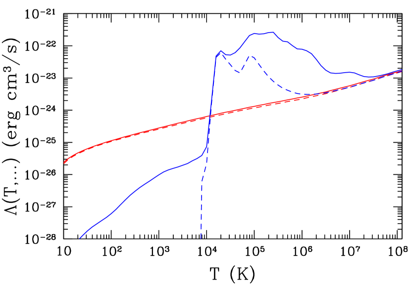
Figure 1.— Example of the importance of the incident radiation field on the cooling functions: blue dashed and solid lines show the “standard cooling function” for the metal-free and solar-metallicity gas respectively. Corresponding red lines show the same cooling functions for the fully ionized gas.

Such dependence can be illustrated by comparing the pure CIE cooling function with the cooling function in fully ionized gas, as shown in Figure 1 for both metal-free and solar-metallicity gas. In the fully-ionized limit, where the only cooling process is bremsstrahlung, the cooling function over a wide range of temperatures differs from a pure CIE case by more than two orders of magnitude!

Thus, the cooling function for photoionized gas depends not only on the gas temperature, number density, and metallicity, but also on the incident radiation field. There is, of course, nothing new in that statement. The crucial role of the radiation environment has always been understood by practitioners in the field. The challenge, however, is in economically accounting for this dependence in full 3D numerical simulations, where the cooling and heating functions are evaluated billions or even trillions of times during a single simulation. In the worst case scenario – the radiation field $J_{\nu}$ varies arbitrarily – one can introduce sharp edges and features in the radiation spectrum that are specially designed to ionize particular levels of particular elements. This allows the cooling function to be “sculpted” in an essentially arbitrary way.

One possible way to account for the effect of the incident radiation field is to fix the radiation spectrum and amplitude. For example, in studies of intergalactic medium it is often (but not always) sufficient to account for the cosmic background radiation. Since the cosmic background radiation evolves with redshift, the cooling and heating functions become redshift-dependent, but such 1-dimensional dependence is easy to pre-compute and tabulate for use in simulations (Benson et al., 2002; Kravtsov, 2003; Wiersma et al., 2009; Vasiliev, 2011). Unfortunately, these cooling and heating rates are then often used for modeling gas dynamics in galactic halos or even ISM – environments where the cosmic background radiation is a sub-dominant component of the incident radiation field.

Therefore, it is desirable to find a way to account for a general shape of the incident radiation field without the need to recompute the cooling and heating functions every time they are needed. In this paper, we show that it is possible to come up with an approximate solution for this problem using a sufficiently general model for the radiation field spectrum.

2. Approximating the Cooling and Heating Functions

The radiative term in the internal energy equation - the rate of change of the gas internal energy due to radiative gains and losses - can be represented as

$$\left.\frac{dU}{dt}\right|_{\rm rad}=n_{b}^{2}\left[\Gamma(T,...)-\Lambda(T,...)\right],$$ (1)

where $U$ is the gas thermal energy and $n_{b}=n_{\rm H}+4n_{\rm He}+..$ is the total baryon number density. We explicitly factored out $n_{b}^{2}$ in both the cooling ($\Lambda$) and the heating ($\Gamma$) functions so that these are density-independent in the CIE limit.

In the most general case the cooling and heating functions depends on an extremely large set of arguments: gas temperature $T$, baryon number density $n_{b}$ (in addition to $n_{b}^{2}$ dependence explicitly accounted for in Equation (1)), the fractional abundance $X_{ij}$ for the species $i$ (including atomic and ionic species, various molecules, and cosmic dust) at level $j$, the distribution of the column density for the species $i$ at level $j$ at different velocity values with respect to the systemic velocity $dN_{ij}(v)/dv$, the specific intensity of the radiation field as a function of frequency $J_{\nu}$, and the heating rate by cosmic rays $\zeta_{\rm CR}$,

$${\cal F}(T,...)={\cal F}\left(T,n_{b},X_{ij},\frac{dN_{ij}(v)}{dv},J_{\nu},\zeta_{\rm CR}\right),$$ (2)

where hereafter ${\cal F}$ denotes either $\Gamma$ or $\Lambda$,

$${\cal F}(...)\equiv\left[\begin{array}[]{l}\Gamma(...)\phantom{\int}\\ \Lambda(...)\phantom{\int}\end{array}\right..$$

Obviously, such a complex dependence cannot be described in simple terms, and would require a detailed calculation with a large set of chemical species using a radiative transfer code - for example, the well-known code Cloudy (Ferland et al., 1998). That would make it impractical as a method for computing the cooling and heating function in realistic three-dimensional numerical simulations.

We, therefore, adopt several major simplifications. First, we restrict our focus to a purely optically thin case (all $N_{ij}=0$). Second, we exclude cooling and heating due to molecules, dust, and cosmic rays, since these processes crucially depend on radiative transfer and computing them in the optically thin limit does not make much physical sense.

With these restrictions, Equation (2) becomes

$${\cal F}(T,...)={\cal F}(T,n_{b},X_{ij},J_{\nu}).$$

Even this is way too complex, as the cooling and heating functions depend on hundreds of individual level populations for atomic and ionized species.

In the next simplification step we assume that all atoms and ions are in the ionization equilibrium, and the level population is in the equilibrium as well. This assumption is actually valid in a vast majority of astrophysical environments. In the limit of ionization equilibrium, the cooling and heating functions only depend on the total abundance of each chemical element. Finally, if we assume that the abundance pattern for heavy elements is solar, and ignore small variations of helium abundance, then the cooling and heating functions become just functions of the gas metallicity,

$${\cal F}(T,...)={\cal F}(T,n_{b},Z,J_{\nu}).$$ (3)

Often, Equation (3) is what is actually called “cooling” and “heating functions”. For example, the CIE cooling and heating functions are just

$${\cal F}_{\rm CIE}(T,Z)={\cal F}(T,n_{b},Z,0)$$

(which, in this limit, is also independent of $n_{b}$).

At low enough densities and faint enough incident radiation fields, most of reactions that result in cooling and heating in gas are interactions of an atom/ion with either a photon or an electron. Hence, in this limit cooling and heating functions (Eq. 1) can be substantially simplified:

$${\cal F}(T,n_{b},Z,J_{\nu})\approx\left.{\cal F}(T,Z,\frac{J_{\nu}}{n_{b}})\right|_{n_{b},J_{\nu}\rightarrow 0}.$$

Unfortunately, this approximation is only valid for rather low values of the radiation field; for example, it is only marginally valid in typical ISM conditions in the Milky Way. Several physical processes break the ideal density-squared dependence. At high enough densities various 3-body processes become important – in particular, 3-body recombination can become important at low temperatures for densities as low as $10^{-4}\mbox{\,cm}^{-3}$. For hard enough incident radiation spectra secondary ionizations and heat deposition from secondary electrons introduce complex density dependence. For strong enough radiation fields some of highly excited energy levels have critical densities within the density range we consider here ($n_{b}\leq 10^{6}\mbox{\,cm}^{-3}$).

All of these processes, however, are relatively smooth functions of the density at a constant value of $J_{\nu}/n_{b}$. Hence, without any loss of generality, we can re-write Equation (3) as

$${\cal F}(T,...)={\cal F}(T,Z,\frac{J_{\nu}}{n_{b}},n_{b}).$$ (4)

The advantage of this transformation is that the third argument includes most of the density dependence; the explicit density dependence parametrized by the fourth argument is relatively weak and can be accounted for in a numerical implementation in an economic manner (the fact we take a full advantage of below).

Finally, we exclude from our cooling and heating functions Compton cooling and heating and free-free absorption - not because they violate the ansatz (4), but because we found empirically that the functional dependence of those two processes on the properties of the medium is sufficiently different from the characteristic dependence of line excitation and emission, so that numerical approximations that we discuss below become substantially less accurate with those two processes included. In addition, Compton processes and free-free absorption depend on the whole shape of the radiation spectrum, even in the low energy regime that is unimportant for the line excitation and ionization. These two processes are described by sufficiently simple analytical expressions that can be easily added separately to a numerical code if there is such a need.

3. Modeling Cooling and Heating Functions and the Incident Radiation Field

As we mentioned above, it is not possible to account parametrically for an arbitrary radiation field spectrum. However, in many astrophysical applications the incident radiation field is dominated by radiation from stars, AGN or a combination thereof. Thus, we model the incident radiation field as

$$J_{\nu}=J_{0}e^{-\tau_{\nu}}\left[\frac{1}{1+f_{Q}}s_{\nu}+\frac{f_{Q}}{1+f_{Q}}x^{-\alpha}\right],$$ (5)

where $x$ is the photon energy in Rydbergs ($x\equiv h\nu/(1\mbox{\,Ry})$), and $s_{\nu}$ is a fit to the stellar spectrum from Starburst99 (Leitherer et al., 1999),

$$s_{\nu}=\frac{1}{5.5}\begin{cases}5.5,&x<1\\ x^{-1.8},&1<x<2.5\\ 0.4x^{-1.8},&2.5<x<4\\ 2\times 10^{-3}x^{3}/\left(\exp(x/1.4)-1\right),&4<x\end{cases}$$

(this fit is shown in Fig. 4 of Ricotti et al. (2002)). Equation (5) also includes the possibility that the incident radiation field is attenuated by gas with the opacity

$$\tau_{\nu}=\frac{\tau_{0}}{\sigma_{{\rm H\,I},0}}\left[0.76\sigma_{\rm H\,I}(\nu)+0.06\sigma_{\rm He\,I}(\nu)\right],$$

where $\sigma_{j}(\nu)$ and $\sigma_{j,0}$ are photoionization cross-sections and their values at respective ionization thresholds for $j={\rm H\,I}$ and ${\rm He\,I}$, and $\tau_{0}$ is a parameter.

Overall, the radiation field model from Equation (5) contains 4 parameters: the amplitude $J_{0}$, the AGN-like power-law contribution slope $\alpha$, the ratio of the AGN-like to stellar component $f_{Q}$, and the shielding optical depth parameter $\tau_{0}$. The last 3 parameters are dimensionless; we choose to measure $J_{0}$ in units of the typical radiation field in the Milky Way galaxy, $J_{\rm MW}=10^{6}\mbox{\,photons}\,\mbox{\,cm}^{-2}\,\mbox{\,s}^{-1}\,\mbox{\,ster}^{-1}\,\mbox{\,eV}^{-1}$ (Draine, 1978; Mathis et al., 1983).

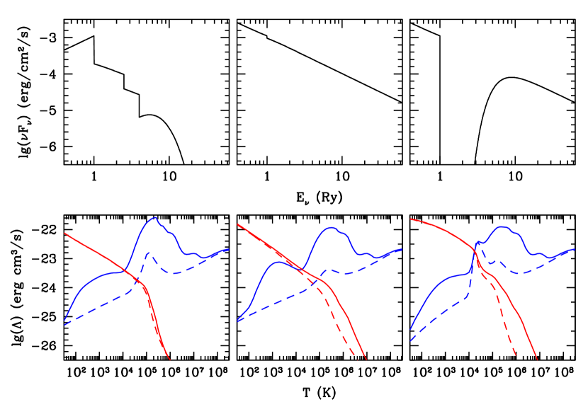
Figure 2.— Incident radiation fields (top panels) and gas cooling (blue lines) and heating (red lines) functions (bottom panels) for three different radiation field models: $[J_{0},\alpha,f_{Q},\tau_{0}]=[100J_{\rm MW},3,10^{-3},0.1]$ (left), $[100J_{\rm MW},2,10,0.1]$ (middle), and $[100J_{\rm MW},2,10,100]$ (right), all for $n_{\rm H}=1\mbox{\,cm}^{-3}$. As in Fig. 1, solid and dashed lines are for $Z=Z_{\odot}$ and $Z=0$ respectively. It is clear that the cooling and heating functions are strongly dependent on the incident radiation field.

For each set of parameters, we use the widely known photoionization code Cloudy (Ferland et al., 1998) to compute the cooling and heating function for a range of gas temperatures at fixed gas density and metallicity. Examples of such computations are shown in Figure 2. For all 3 cases the radiation field is the same at $1\mbox{\,Ry}$, but differs in spectral shape at other frequencies (a stellar spectrum, a power-law spectrum, and a power-law spectrum shielded by a $\tau_{0}=100$ cloud). In order to enforce the optically thin case, we restrict Cloudy calculations to a single zone of a negligibly small size.

We explore the cooling and heating functions for our radiation field model by sampling the full parameter space (metallicity, density, and the radiation field) on the following grid of values:

$$Z/Z_{\odot} = 0,0.1,0.3,1,3$$

$$\lg(n_{b}/\mbox{\,cm}^{-3}) = -6,-5,...,6$$

$$\lg(J_{0}\mbox{\,cm}^{-3}/n_{b}/J_{\rm MW}) = -5,-4.5,-4,...,7$$

$$\alpha = 0,0.5,1,1.5,2,2.5,3$$ (6)

$$\lg(f_{q}) = -3,-2.5,-2,...,1$$

$$\lg(\tau_{0}) = -1,-0.5,0,...,3$$

This parameter range is wide enough to include both extremes shown in Fig. 1: the case where the radiation field is completely negligible and the case where the gas is fully photoionized.

For each of the $5\times 13\times 25\times 7\times 9\times 9\approx 920{,}000$ sets of parameters from this grid, we run Cloudy to compute the cooling and heating functions for 81 values of the temperature between $10\mbox{\,K}$ and $10^{9}\mbox{\,K}$ in steps of $0.1\mbox{\,dex}$ (almost 75 million Cloudy runs altogether). Using this large database, we now consider the various dependencies of the cooling and heating functions one by one. All of our subsequent approximations are extensively tested below in §4.

3.1. Metallicity and Density Dependence

In a further simplification, we expand both cooling and heating functions into Taylor series in metallicity up to the quadratic term,

$${\cal F}\approx{\cal F}_{0}+\frac{Z}{Z_{\odot}}{\cal F}_{1}+\left(\frac{Z}{Z_{\odot}}\right)^{2}{\cal F}_{2},$$ (7)

where all functions ${\cal F}_{i}$ depend only on $T$, $J_{\nu}/n_{b}$, and $n_{b}$.

We achieve this decomposition in practice by fitting a second degree polynomial to the five $Z$ values that we sample in Table (6). The error introduced by dropping cubic and higher power terms is by far the smallest of the errors introduced by our approximations – in the rms sense, the second order expansion of the Taylor series is accurate to better than 3% – as long as we restrict $Z$ to less than 3 solar metallicities. The quadratic approximation rapidly loses accuracy as the metallicity increases. At metallicities above $5Z_{\odot}$, approximation (7) even results in negative cooling functions in a few instances.

Six functions $\Gamma_{i}$ and $\Lambda_{i}$ ($i=0,1,2$) can be used directly, but since cooling and heating functions are not necessarily monotonic functions of $Z$, some of ${\cal F}_{1}$ and ${\cal F}_{2}$ (again, ${\cal F}$ stands for either $\Gamma$ or $\Lambda$) can be negative. Since interpolation in log-log space is usually more accurate than direct interpolation, positive functions are much more suitable for tabulation and interpolation. Hence, we replace 6 functions ${\cal F}_{i}$ with 6 new functions $\tilde{\cal F}_{i}$ as

$$\tilde{\cal F}_{0} = {\cal F}_{0},$$

$$\tilde{\cal F}_{1} = {\cal F}_{0}+{\cal F}_{1}+{\cal F}_{2},$$

$$\tilde{\cal F}_{2} = {\cal F}_{0}+2{\cal F}_{1}+4{\cal F}_{2},$$

where symbol $\tilde{\cal F}$ also means either the cooling or the heating function. Functions $\tilde{\cal F}_{i}$ are none other than the cooling and heating functions at $Z=i\times Z_{\odot}$ and hence are always positive. The transformation between ${\cal F}_{i}$ and $\tilde{\cal F}_{i}$ is linear and can be trivially inverted.

In the following, we always operate on functions $\tilde{\cal F}_{i}$ and convert them back to ${\cal F}_{i}$ (i.e. $\Gamma_{i}$ and $\Lambda_{i}$) as the very last step.

3.2. Radiation Field Dependence

So far we still have not resolved the main challenge – the fact that the 6 functions $\tilde{\cal F}_{i}$ that we need to describe depend on the whole incident radiation field $J_{\nu}$,

$$\tilde{\cal F}_{i}=\tilde{\cal F}_{i}(T,\frac{J_{\nu}}{n_{b}},n_{b}).$$

The primary contribution of this paper is that we further approximate this dependence by replacing the full radiation field with a finite set of photoionization rates.

Specifically, let us define a normalized rate $Q_{j}$ as

$$Q_{j}\equiv\frac{P_{j}}{n_{b}},$$

where $P_{j}$ is a photoionization rate for some atom or ion,

$$P_{j}=c\int_{0}^{\infty}\sigma_{j}(\nu)n_{\nu}d\nu,$$

where $\sigma_{j}$ is the photoionization cross-section and $n_{\nu}$ is the radiation field expressed as the number density of photons at the frequency $\nu$. We now seek an approximation of the form

$$\tilde{\cal F}_{i}(T,\frac{J_{\nu}}{n_{b}},n_{b})\approx\tilde{\cal F}_{i}(T,Q_{j},n_{b})$$ (8)

for $i=0,1,2$ and some set of $Q_{j}$. If such an approximation is possible, then a user would only need to compute the (normalized) photoionization rates $Q_{j}$ from his/her assumed radiation field (provided, such a field is close enough to our assumed shape - as we mentioned above, it is always possible to sculpt the cooling and heating functions by appropriate choosing the radiation field spectrum).

We present our specific choice for $Q_{j}$ in §3.4.

3.3. Explicit Density Dependence

Finally, we need to address the remaining density dependence in Equation (8). The trick of using $Q_{j}$ makes this dependence relatively weak, although highly non-trivial. We adopt the simplest possible approach – we tabulate $\tilde{\cal F}_{i}$ at the 13 density values we tested in Table (6) and linearly interpolate in log-log space. The guaranteed positiveness of $\tilde{\cal F}_{i}$ becomes crucial when working in logarithmic space.

We verified that the error introduced by such interpolation is completely sub-dominant to the error of our main approximation (8).

3.4. Notes on the Specific Implementation

It makes sense that the rates we choose to represent the radiation field should sample the wide range of frequencies. For example, since ${\rm C\,II}$ is an important coolant in the low-temperature regime, one of the rates should sample the radiation field below the hydrogen ionization threshold. We choose the photodissociation rate of molecular hydrogen in the Lyman-Werner band as such a rate, simply because that rate is also useful for several other processes that can be modeled in the numerical code (for example, the destruction of molecular hydrogen). It also makes sense to use the hydrogen and helium ionization rates since both elements are important coolants at $T\gtrsim 10{,}000\mbox{\,K}$ for all but the highest radiation fields. Finally, one of the selected rates should be sensitive to high energy photons.

While it is not possible to explore the full set of some 600+ photoionization rates for common chemical elements, we searched the full hydrogen-like sequence all the way to ${\rm Fe\,XXVI}$ for the most accurate approximation for the cooling and heating functions.

For a practical numerical implementation, a table with cooling and heating functions should not exceed about 1 GB of memory, and a much smaller memory footprint is much preferred. Most modern supercomputers offer between 1 and 2 GB of memory per computing core; a 1 GB table would leave no memory for other data structures in a pure MPI code on a 1 GB/core machine. While pure MPI codes are getting more and more rare, even a hybrid code that uses just one MPI task per an 8-core node with 8 GB of memory would encounter difficulty using a table in excess of 1 GB.

With these constraints in mind, we explored a wide range of possible 3- and 4-dimensional tables. We have not found a 4-dimensional solution that is sufficiently superior to our best 3-dimensional table and that fits within our imposed 1 GB memory limit.

Hence, as our primary implementation, we present a 3-dimensional table that is constructed from four normalized photoionization rates, $Q_{\rm LW}$, $Q_{\rm H\,I}$, $Q_{\rm He\,I}$, and $Q_{\rm C\,VI}$, combined into 3 independent parameters,

$$r_{1} = Q_{\rm LW},$$

$$r_{2} = \left(\frac{Q_{\rm H\,I}}{Q_{\rm LW}}\right)^{0.353}\left(\frac{Q_{\rm He\,I}}{Q_{\rm LW}}\right)^{0.923}\left(\frac{Q_{\rm C\,VI}}{Q_{\rm LW}}\right)^{0.263},$$

$$r_{3} = \left(\frac{Q_{\rm H\,I}}{Q_{\rm LW}}\right)^{-0.103}\left(\frac{Q_{\rm He\,I}}{Q_{\rm LW}}\right)^{-0.375}\left(\frac{Q_{\rm C\,VI}}{Q_{\rm LW}}\right)^{0.976}.$$ (9)

There exist several other combinations of various rates that result in almost equivalent approximations. For example, adding $Q_{\rm Mg\,XII}$ as a fifth rate reduces the error of the approximation by about 0.03 dex - not significant enough, in our opinion, to justify computing an extra photoionization rate.

We implement the approximation (8) by constructing a grid of $r_{j}$ values and computing the average cooling and heating functions for all incident radiation fields that happen to have the same values for $r_{j}$. Specifically, we use a logarithmically-spaced table for $-14.5\leq\lg(r_{1})\leq-3$, $-9.5\leq\lg(r_{2})\leq 0.5$, and $-8\leq\lg(r_{3})\leq-0.5$ with the logarithmic step of $0.5\mbox{\,dex}$. We found that using a finer step in the table does not lead to any increase of accuracy. Such a table includes $24\times 21\times 16=8064$ entries; each entry contains a sub-grid of 13 density values by 81 temperature values, with 6 numbers ${\cal F}_{i}$ at each grid point. A full table takes about 192 MB of memory. The table can be further compressed by eliminating entries with similar cooling and heating functions, to the total of 3795 entries (92 MB of memory).

With these memory requirements, the final table can be used even in purely MPI codes on low memory platforms.

4. Testing the Complete Approximation

Since we use our sample of Cloudy runs to create the actual tables with the cooling and heating functions, we need a different data set to test the accuracy of our approximations. For this purpose we select 100,000 points from within our parameter space (6), sampled uniformly on a logarithmic scale (for the metallicity, we randomly choose a value between -3 and 0.5 in $\lg(Z)$). For each test point, we run Cloudy for our 81 values of the temperature to compute cooling and heating functions. This “testing” data set is completely independent of the data set used to create the tables.

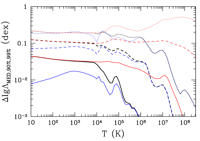
Figure 3.— Error in approximating the cooling (blue lines), heating (red lines), and the maximum of the two (black lines) functions with several photoionization rates. Solid lines trace the median error (50% of cases have the error below the solid line), dashed lines trace the 90% error, and dotted line trace the 99% error (only 1% of all cases have an error above the dotted line). The existence of “catastrophic” errors (a small number of cases with large errors) is apparent from this figure.

We show in Figure 3 the error distribution for our primary implementation described above. While errors of both functions can be evaluated, in practice only the difference between the heating and cooling functions matters (Equation 1) - i.e., if one of the two functions is much larger than the other, a bigger error can be tolerated for the smaller of the two. Thus, we also show in Figure 3 the error of the largest of the two functions at each temperature - that error is a more suitable measure of the actual error of our approximation.

Two features of Fig. 3 are important to note. First, the median errors for both cooling and heating functions are modest, less than 10%. This is very good news indeed, as it shows that the whole diversity of cooling and heating functions can be parametrized economically, albeit approximately. Second, unfortunately, is that the error distribution is not Gaussian, but rather exhibits a long tail toward large, or “catastrophic”, errors. For example, in 0.1% of all cases that we tested, the error of our approximation reaches a factor of 2.

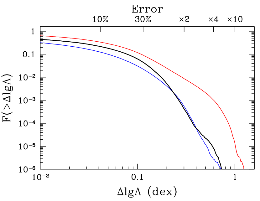
Figure 4.— Cumulative error distributions for all values of gas temperatures for the heating (red line), cooling (blue line), and the maximum of the two (black line) functions for our approximation.

This property of our approximation is further illustrated in Figure 4, where we show the cumulative error distribution for all temperature values separately for the cooling function, the heating function, and the maximum of the two (the most appropriate measure of the actual error). For one case in a million, our approximation reaches an error of about a factor of 6. Of course, the specific shapes of the distributions shown in Fig. 3 and 4 are only applicable to our adopted uniform sampling. For a specific numerical simulation, the probability of errors of a particular magnitude will depend on the simulation details (such as temperature, density, metallicity, and the radiation field PDFs) and cannot be predicted a priori.

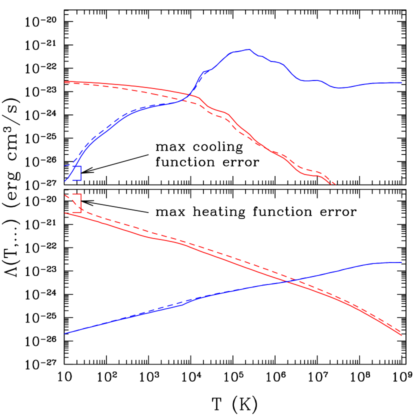
Figure 5.— Cooling (blue lines) and heating (red lines) functions for our test models that maximize the error in the cooling function (top panel) and the heating function (bottom panel). Approximate functions extracted from our table are shown as dashed lines, while actual calculation from Cloudy are shown with solid lines.

In order to further illustrate the appearance of a “catastrophic error”, we show in Figure 5 the actual cooling and heating functions that maximize the errors (out of 100,000 samples of 81 temperature values each) in both the heating and cooling functions. These errors occur in different regions of the parameter space (i.e. the worst-case heating function is not the heating function that corresponds to the worst-case cooling function, and vice versa). In most cases that we were able to examine manually, the largest errors occur at either very low or very high temperatures, very far from the thermal equilibrium values.

More good news is that the large errors typically occur within a narrow range of temperatures, like in Fig. 5. Hence, as soon as the gas temperature changes in the simulation code, the error in the cooling and heating functions is likely to fall appreciably. For example, in the bottom panel of Fig. 5 the error in the heating function is a factor of 6 for $T=10\mbox{\,K}$. The heating function is very large, so the gas in this state is going to get heated to higher temperature rapidly, trying to reach the thermal equilibrium at $T\approx 2\times 10^{6}\mbox{\,K}$. As soon as the gas temperature increases to $T\sim 100\mbox{\,K}$, the error in our approximation drops to less than a factor of 2 (for the fixed values of the normalized photoionization rates $Q_{j}$), and will remain within that range until the thermal equilibrium is reached.

While our adopted spectral shape (5) is sufficiently reasonable, it does not represent many situations of astrophysical interest. In order to test how our approximation fares for other radiation fields, we apply it to several spectral shapes that are built-in into Cloudy. Specifically, for each of the built-in spectral shapes, we randomly choose a value of the density within our full range $-6\leq\lg(n_{b}/\mbox{\,cm}^{-3})\leq 6$, randomly scale the radiation field by a factor between $10^{-3}$ and $10^{3}$ (except for the Haardt-Madau 2005 background, for which we randomly choose a value of cosmic redshift between 0 and 6), use Cloudy to compute the actual cooling and heating functions for that set of parameters, and then compare Cloudy results with the cooling and heating functions returned by our approximation when we use the actual photoionization rates that Cloudy reports for the chosen spectral shape.

Figure 6.— Cumulative error distributions for all values of gas temperatures for the maximum of the cooling and heating functions for other spectral shapes that are built-in into Cloudy: Milky Way ISM (Cloudy command “table ISM”, dotted line), typical AGN spectrum (Cloudy command “table AGN”, short-dashed line), Haardt-Madau 2005 cosmic background for $z<4$ (Cloudy command “table HM05”, long-dashed line), Haardt-Madau 2005 cosmic background for $z>4$ (Cloudy command “table HM05”, dot-short-dashed line), continuum from the Crab nebula (Cloudy command “table Crab”, dot-long-dashed line), and continuum from a cooling flow (Cloudy command “table Cooling Flow”, short-dash-long-dashed line). We also show with the solid line the black line from Fig. 4 for comparison.

The cumulative error distribution for several built-in spectral shapes is shown in Figure 6. In all cases except one the maximum error of our approximation does not exceed a factor of 3, and the error distribution falls off sharply at large errors - in fact, more sharply than the error distribution for our chosen spectral shape from Equation (5); this is not an artifact of incomplete sampling - we run enough Cloudy models for each spectral shape to sample the error distribution all the way down to $10^{-6}$.

The only case where our approximation fares worse, producing a significant fraction ($10^{-3}$) errors as large as a factor of 5, is the case of the Haardt-Madau 2005 cosmic background for $z>4$. This is rather disappointing, as cosmological simulations are intended to be the primary user of our approximation, but we have not succeeded in finding an approximation that has a noticeably lower error for that case.

5. Conclusions

Our main result is that one can approximately represent the most general cooling and heating functions for gas in ionization equilibrium as

$$\left\{\Gamma,\Lambda\right\}(T,n_{b},Z,J_{\nu})\approx\sum_{i=0}^{2}\left(\frac{Z}{Z_{\odot}}\right)^{i}\left\{\Gamma,\Lambda\right\}_{i}(T,r_{j},n_{b}),$$ (10)

where $r_{j}$ are given in Equation (9). This approximation is rather accurate on average, but suffers from “catastrophic” errors – in $10^{-6}$ of all cases the approximate cooling or heating function may deviate from the exact calculation by up to a factor of 6. Thus, our approximation is not suitable for all applications.

Equation (10) does capture the qualitative dependence of the cooling and heating functions on the incident radiation field. To illustrate this, we show in the appendix three examples where the cooling and heating functions are significantly modified by the incident radiation field. The last example – the quasar irradiating its own galactic halo (§A.3) – not only shows a large effect the radiation field can have on the cooling/heating functions, but actually presents an alternative feedback mechanism: the central black hole suppresses the gas accretion from the halo without any additional mechanical or thermal feedback.

Our data table and the reader code for it are available online at http://astro.uchicago.edu/$\sim$gnedin

Appendix A Some Examples of Cooling and Heating Functions in ISM and IGM

In this section we present a few examples where the incident radiation field significantly affects the cooling and heating rates in the gas. These examples are not real physical models, but are simple demonstrations that the dependence that we explore in this paper actually matters.

The examples presented here are not exhaustive, of course; one can imagine many other similar situations. Their purpose is to illustrate the numerous possible feedback effects in interstellar and intergalactic environments that arise when we take into account the effects of the gas metallicity and the incident radiation field on the cooling and heating rates. These effects can be studied, even if only approximately, with the approximations presented in this paper.

A.1. Galactic Halo Near a Quasar

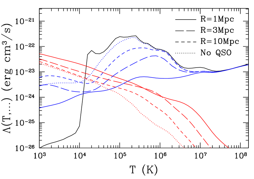
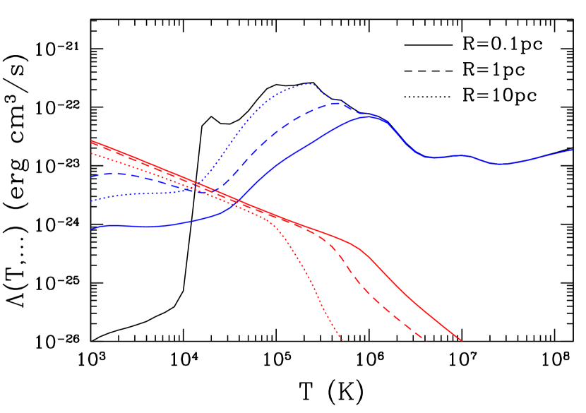
Figure 7.— Left: Cooling (blue lines) and heating (red lines) functions for a $Z=Z_{\odot}$, $n_{b}=340\times\bar{n}_{b}$ galactic halo at the specified distances from a quasar with an ionizing luminosity $10^{13}L_{\odot}$. The black solid line shows the pure CIE “standard cooling function”. Right: Cooling (blue lines) and heating (red lines) functions for a $Z=Z_{\odot}$, $n_{b}=1\mbox{\,cm}^{-3}$ ${\rm H\,II}$ region around an O star. The black solid line shows the pure CIE “standard cooling function”.

In the left panel of Figure 7 we show cooling and heating functions for a typical galactic halo at $z=0$ ($n_{b}=340\times\bar{n}_{b}=8.5\times 10^{-5}\mbox{\,cm}^{-3}$) surrounding a bright quasar with an ionizing luminosity of $10^{13}L_{\odot}$ (roughly corresponding to a $10^{9}M_{\odot}$ black hole). We assume solar metallicity, a quasar spectrum of $J_{\nu}\propto\nu^{-2}$, and the Haardt & Madau (2001) background.

Some interesting consequences may arise from the radiation-field-dependence of the cooling and heating functions. For example, gas in the halo within $1\mbox{\,Mpc}$ of this quasar will not be able to cool and condense into the disk if its virial temperature is below about $10^{5}\mbox{\,K}$.

A.2. ${\rm H\,II}$ Region Around an O Star

In the right panel of Figure 7, we show the cooling and heating functions for a solar metallicity cloud with density $n_{b}=1\mbox{\,cm}^{-3}$ surrounding an O star with bolometric luminosity $L=30{,}000L_{\odot}$. For the stellar spectrum, we assume a black-body with $T=30{,}000\mbox{\,K}$. The distances we consider are well within the star’s Strömgren radius ($\sim 30\mbox{\,pc}$), so we may safely assume that the radial dependence of the starlight is $1/r^{2}$ (no depletion due to recombinations). If, instead of a single star, we consider a cluster of $N$ O stars, our result will still hold if we simply rescale the distance axis by $N^{1/2}$.

Close enough to the star, the equilibrium temperature of the ${\rm H\,II}$ region can be substantially higher than the canonical $10^{4}\mbox{\,K}$.

A.3. Quasar Irradiating its own Halo

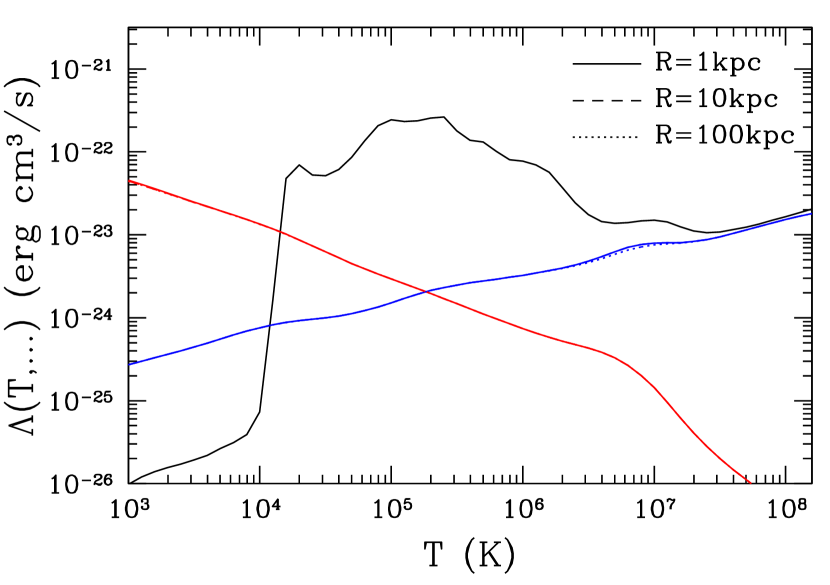
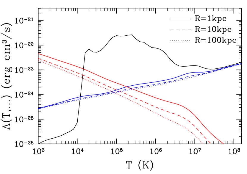
Figure 8.— Cooling (blue lines) and heating (red lines) curves for a halo with a $z=3$ isothermal density profile surrounding a quasar with $10^{13}L_{\odot}$ in ionizing radiation. In the left panel, the metallicity is fixed at $0.5Z_{\odot}$, in which case the cooling and heating functions become distance-independent. In the right panel, the metallicity has a mild outward gradient, $Z\propto r^{-1/2}$. The black solid curves show the pure CIE “standard cooling function”.

In Figure 8 we show cooling and heating functions in a gaseous halo at $z=3$ (virial density $n_{b}=200\times\bar{n}_{b}=3.2\times 10^{-3}\mbox{\,cm}^{-3}$) irradiated by a $\sim 10^{9}M_{\odot}$ central black hole ($10^{13}L_{\odot}$ in ionizing radiation). The density profile of the cloud is taken as

$$n_{b}=3.2\times 10^{-3}\mbox{\,cm}^{-3}\left(\frac{100\mbox{\,kpc}}{r}\right)^{2}$$

and the metallicity is taken either to be constant $0.5Z_{\odot}$ (leading to distance-independent heating and cooling functions) or to have a mild outward gradient,

$$Z=0.5Z_{\odot}\left(\frac{1\mbox{\,kpc}}{r}\right)^{1/2}.$$

In both cases, the quasar is capable of maintaining the heating rate in excess of the cooling rate for $T\lesssim 10^{5}\mbox{\,K}$. It is therefore possible to prevent cooling in the halo – and hence, accretion of fresh gas onto the galactic disk and the black hole – without any need for a mechanical or non-radiative thermal feedback mechanism. This result is, of course, not new (Sazonov et al., 2005; Ciotti & Ostriker, 2007), here we simply use it as an illustration to the importance of properly accounting for the radiation field dependence of the cooling and heating functions.

References

- Benjamin et al. (2001) Benjamin, R. A., Benson, B. A., & Cox, D. P. 2001, ApJ, 554, L225
- Benson et al. (2002) Benson, A. J., Lacey, C. G., Baugh, C. M., Cole, S., & Frenk, C. S. 2002, MNRAS, 333, 156
- Boehringer & Hensler (1989) Boehringer, H. & Hensler, G. 1989, A&A, 215, 147
- Ciotti & Ostriker (2007) Ciotti, L. & Ostriker, J. P. 2007, ApJ, 665, 1038
- Cox & Tucker (1969) Cox, D. P. & Tucker, W. H. 1969, ApJ, 157, 1157
- Draine (1978) Draine, B. T. 1978, ApJS, 36, 595
- Ferland et al. (1998) Ferland, G. J., Korista, K. T., Verner, D. A., Ferguson, J. W., Kingdon, J. B., & Verner, E. M. 1998, PASP, 110, 761
- Gaetz & Salpeter (1983) Gaetz, T. J. & Salpeter, E. E. 1983, ApJS, 52, 155
- Gnat & Sternberg (2007) Gnat, O. & Sternberg, A. 2007, ApJS, 168, 213
- Haardt & Madau (2001) Haardt, F. & Madau, P. 2001, in Clusters of Galaxies and the High Redshift Universe Observed in X-rays, ed. D. M. Neumann & J. T. V. Tran
- Kravtsov (2003) Kravtsov, A. V. 2003, ApJ, 590, L1
- Landi & Landini (1999) Landi, E. & Landini, M. 1999, A&A, 347, 401
- Leitherer et al. (1999) Leitherer, C., Schaerer, D., Goldader, J. D., Delgado, R. M. G., Robert, C., Kune, D. F., de Mello, D. F., Devost, D., & Heckman, T. M. 1999, ApJS, 123, 3
- Mathis et al. (1983) Mathis, J. S., Mezger, P. G., & Panagia, N. 1983, A&A, 128, 212
- Raymond et al. (1976) Raymond, J. C., Cox, D. P., & Smith, B. W. 1976, ApJ, 204, 290
- Ricotti et al. (2002) Ricotti, M., Gnedin, N. Y., & Shull, J. M. 2002, ApJ, 575, 33
- Santoro & Shull (2006) Santoro, F. & Shull, J. M. 2006, ApJ, 643, 26
- Sazonov et al. (2005) Sazonov, S. Y., Ostriker, J. P., Ciotti, L., & Sunyaev, R. A. 2005, MNRAS, 358, 168
- Shull & van Steenberg (1982) Shull, J. M. & van Steenberg, M. 1982, ApJS, 48, 95
- Smith et al. (2008) Smith, B., Sigurdsson, S., & Abel, T. 2008, MNRAS, 385, 1443
- Sutherland & Dopita (1993) Sutherland, R. S. & Dopita, M. A. 1993, ApJS, 88, 253
- Vasiliev (2011) Vasiliev, E. O. 2011, MNRAS, 414, 3145
- Wiersma et al. (2009) Wiersma, R. P. C., Schaye, J., & Smith, B. D. 2009, MNRAS, 393, 99