Connecting Solutions in Open String Field Theory with Singular Gauge Transformations

Theodore Erler^(a)

Carlo Maccaferri^(a,b)

^(a)Institute of Physics of the ASCR, v.v.i.
Na Slovance 2, 182 21 Prague 8, Czech Republic

^(b)INFN, Sezione di Torino
Via Pietro Giuria 1, I-10125 Torino, Italy
Abstract

We show that any pair of classical solutions of open string field theory can be related by a formal gauge transformation defined by a gauge parameter $U$ without an inverse. We investigate how this observation can be used to construct new solutions. We find that a choice of gauge parameter consistently generates a new solution only if the BRST charge maps the image of $U$ into itself. When this occurs, we argue that $U$ naturally defines a star algebra projector which describes a surface of string connecting the boundary conformal field theories of the classical solutions related by $U$. We also note that singular gauge transformations give the solution space of open string field theory the structure of a category, and we comment on the physical interpretation of this observation.

1 Introduction

Classical solutions in Chern-Simons-like theories [1, 2] are given by flat connections. The easiest way to find a flat connection is to assume that the solution can be written in the form

$$A=U^{-1}dU.$$ (1.1)

Naively this implies that $A$ is pure gauge. However, the solution can be nontrivial if, for some reason, $U$ is not an acceptable gauge transformation. This can happen in a couple of ways. One way is if the gauge transformation $U$ does not belong to the space of fields used to define the theory. For example, in Chern-Simons theory on a 3-manifold $\mathcal{M}$, we can construct a Wilson line wrapping a noncontractible cycle using a gauge parameter $U$ which lives on the universal cover of $\mathcal{M}$. The string field theory analogue of this is to construct $U$ using an insertion of a boundary condition changing operator, so that $U$ is not a state within a single boundary conformal field theory. This idea is a starting point for the construction of analytic solutions for marginal deformations in open string field theory [3, 4, 5, 6].

However, $U$ can fail to be a gauge transformation for another reason: $U$ might not have an inverse. This is the sense that Schnabl’s solution for the tachyon vacuum is “almost” pure gauge [7, 8]. This suggests an appealingly simple strategy for discovering new solutions: Make an educated guess for $U$, and then solve the linear inhomogeneous equation $QU=U\Phi$ for $\Phi$. This strategy has lead to interesting proposals for the tachyon lump [9, 10] and multiple branes solutions [11, 12], but unfortunately these constructions are singular and it is not known how to make them consistent with the equations of motion [12, 13, 14, 15]. The problem can be traced to the fact that because $U$ is not invertible, in general $U^{-1}QU$ is not well-defined.

In this paper we attempt to confront this issue. First we show that any pair of solutions in open string field theory can be related by a gauge transformation of the form (1.1), with the understanding that $U$ might not be invertible. We call this a left gauge transformation. We then observe that the expression $U^{-1}(Q+\Phi_{1})U$ only makes sense if $(Q+\Phi_{1})U$ is equal to $U$ times something. This imposes a nontrivial constraint on the possible $U$s which can be used to define new solutions. To phrase this condition in a more useful way, we assume the existence of a star algebra projector $X^{\infty}$ which projects onto the left and right kernel of $U$. Then a consistent left gauge transformation must satisfy the constraint:

$$X^{\infty}Q_{\Phi_{1}}U=0.$$ (1.2)

where $Q_{\Phi_{1}}$ is the kinetic operator around the reference solution. Our understanding of this equation is formal, and we will not attempt to solve it to find new solutions in this paper. However, we show that, under a few assumptions, it is nontrivially satisfied for all analytic solutions we have studied, and it is violated for the multibrane and lump solutions of [9, 10, 11, 12], which are known to encounter difficulties. One interesting byproduct of our analysis concerns the projector $X^{\infty}$. By formal arguments and examples, we find that $X^{\infty}$ is a projector-like state representing a surface of open string connecting the boundary conformal field theories of the classical solutions related by $U$. Accordingly, we call $X^{\infty}$ the boundary condition changing projector. The boundary condition changing projector is important not only because of the consistency condition (1.2), but also because it determines the structure of the phantom term needed to precisely define the solution in pure gauge form [7, 8, 16, 17, 18, 19, 20, 21].

This paper is organized as follows. In section 2 we develop the formalism assuming that the string field algebra can be usefully modeled as a (preferably finite dimensional) algebra of operators acting on some vector space. We show how to relate any two classical solutions by a left gauge transformation, state the assumptions needed in order to define the boundary condition changing projector, and state two conditions—the strong and weak consistency conditions—which every singular gauge transformation should satisfy in order to generate a new solution. Computing the BRST variation of $X^{\infty}$, we motivate a physical interpretation of the boundary condition changing projector in terms of a stretched string connecting two boundary conformal field theories. We comment on the relation between the boundary condition changing projector and the characteristic projector defined by Ellwood [9]. Finally we demonstrate the formalism using a finite dimensional toy model of vacuum string field theory. In section 3, we observe that left gauge transformations can be interpreted as the morphisms of a category whose objects are classical solutions. We explain how this structure can be naturally related to a picture of open strings ending on D-branes. In section 4 we apply the formalism to some known analytic solutions in string field theory, finding that, with some assumptions, it does a pretty good job at explaining why some candidate formal gauge transformations define solutions, while others do not. We also work out explicit examples of the boundary condition changing projector and describe how it implements the change of boundary condition. We end with some discussion.

2 Formalism

To set up the formalism, we consider a “model” of the open string star algebra consisting of three ingredients:

1) An associative algebra $\mathcal{A}$ with an integer grading which we call ghost number, and a $\mathbb{Z}_{2}$ grading corresponding to Grassmann parity. Grassmann parity is identified with ghost number mod $\mathbb{Z}_{2}$.

2) A nilpotent, Grassmann odd and ghost number 1 derivation of $\mathcal{A}$ which we call the BRST operator $Q$.

3) A representation of $\mathcal{A}$ as an algebra of operators acting on some vector space, $\mathcal{D}$.

In string field theory, $\mathcal{D}$ might be identified with the space of half-string wavefunctionals [22, 23], but at present it is difficult to say much concrete about this. We will not attempt to be rigorous about the precise analytic definition of the operator algebra $\mathcal{A}$ and its topology; unless otherwise mentioned, we will effectively assume $\mathcal{D}$ is a finite dimensional vector space. This means that, for string field theory purposes, our discussion will be formal. Its relevance should be justified by examples, as discussed in section 4.

Note that ingredients 1)-3) are not specific to string field theory, but can be realized in Chern-Simons [1] or noncommutative Chern-Simons theory [24, 25]. However, as we will see the formalism is less interesting in these examples due to the absence of fields with negative ghost number.

2.1 Left Gauge Transformations

Consider two solutions $\Phi_{1}$ and $\Phi_{2}$ related by a finite gauge transformation:

$$\tilde{U}(Q+\Phi_{1})U=\Phi_{2},$$ (2.1)

where $\tilde{U}U=U\tilde{U}=1$. Multiplying this equation by $U$ from the left, we find the relation

$$(Q+\Phi_{1})U=U\Phi_{2},$$ (2.2)

and multiplying by $\tilde{U}$ from the right gives the equation

$$-Q\tilde{U}+\tilde{U}\Phi_{1}=\Phi_{2}\tilde{U}.$$ (2.3)

We will call $U$ satisfying (2.2) a left gauge transformation from $\Phi_{1}$ to $\Phi_{2}$, and $\tilde{U}$ satisfying (2.3) a right gauge transformation from $\Phi_{1}$ to $\Phi_{2}$. A left gauge transformation from $\Phi_{1}$ to $\Phi_{2}$ is also a right gauge transformation, in reverse, from $\Phi_{2}$ to $\Phi_{1}$. Note that these definitions are meaningful even when $U$ or $\tilde{U}$ are not invertible, in which case $\Phi_{1}$ and $\Phi_{2}$ may not be gauge equivalent solutions. If $U$ or $\tilde{U}$ is invertible, then we will call it a proper gauge transformation, and, if not, singular gauge transformation.

A short explanation of terminology: When discussing left gauge transformations, we will think of operators in the algebra $\mathcal{A}$ as acting from the left on the representation space $\mathcal{D}$. For right gauge transformations, it turns out to be more natural to treat operators as acting from the right on the dual space $\mathcal{D}^{\prime}$. In the following development we will focus on left gauge transformations. The story for right gauge transformations is simply a “mirror image.”

It is convenient to introduce the operator

$$Q_{\Phi_{1}\Phi_{2}}A\equiv QA+\Phi_{1}A+(-1)^{A}A\Phi_{2}.$$ (2.4)

This is nilpotent, but not a derivation. However it satisfies a modified Leibniz rule,

$$Q_{\Phi_{1}\Phi_{3}}(AB)\!\!\!\!\!\!\!\! =(Q_{\Phi_{1}\Phi_{2}}A)B+(-1)^{A}A(Q_{\Phi_{2}\Phi_{3}}B),$$ (2.5)

where $\Phi_{2}$ on the right hand side is any solution. Rewriting (2.2), we can define a left gauge transformation $U$ as a ghost number zero solution to the equation:

$$Q_{\Phi_{1}\Phi_{2}}U=0.$$ (2.6)

The obvious solution is $U=0$, but this is too trivial to be interesting. If the theory has a nonzero field $b$ at ghost number $-1$, we can find a more interesting solution

$$U=Q_{\Phi_{1}\Phi_{2}}b.$$ (2.7)

Since string field theory has many fields with negative ghost number, this implies the following:

$$\phantom{\Bigg{(}}{\mbox{\it In string field theory there is always a nonzero left gauge transformation}\atop\mbox{\it connecting any pair of solutions.}\ \ \ \ \ \ \ \ \ \ \ \ \ \ \ \ \ \ \ \ \ \ \ \ \ \ \ \ \ \ \ \ \ \ \ \ \ \ \ \ \ \ \ \ \ \ \ \ \ \ \ \ }$$

This is not the case in Chern-Simons theory. Since there are no negative rank forms, the construction of nonzero left gauge transformations depends on whether $Q_{\Phi_{1}\Phi_{2}}$ has cohomology at ghost number zero. If $\Phi_{1}$ and $\Phi_{2}$ are gauge equivalent, $Q_{\Phi_{1}\Phi_{2}}$ will have cohomology by construction, but this is not guaranteed if they are not gauge equivalent. Therefore, the existence of nonzero singular gauge transformations is something particularly characteristic of string field theory.

2.2 Consistency Conditions and the BCC projector

The basic question we want to ask is this: Given a solution $\Phi_{1}$, when can a field $U$ be regarded as a left gauge transformation to another solution $\Phi_{2}$? From equation (2.2) it is obvious that that $(Q+\Phi_{1})U$ should be equal to $U$ times something. If the fields are linear operators acting on $\mathcal{D}$, this means

$$\boxed{\phantom{\Bigg{)}}\mathrm{Im}\,Q_{\Phi_{1}}U\subseteq\mathrm{Im}\,U.\ \ \ }$$ (2.8)

In other words, the kinetic operator around the solution $\Phi_{1}$ must map the image of $U$ into itself. We will call this the strong consistency condition. This condition implies that we can find a field $\Phi_{2}$ satisfying $(Q+\Phi_{1})U=U\Phi_{2}$, but it does not guarantee that $\Phi_{2}$ is a solution. However, $\Phi_{2}$ at least satisfies

$$U(Q\Phi_{2}+\Phi_{2}^{2})=0,$$ (2.9)

so it is a solution up to the kernel of $U$.

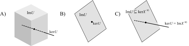
Figure 2.1: We assume that the image and kernel of $U$ are linearly independent and span the whole space, as shown above in case C). In cases A) and B) the image and kernel of $U$ are not linearly independent or do not span the whole space. This would happen if $U$ was a non-unitary isometry.

While the strong consistency condition (2.8) is true, it is not very helpful since checking it seems to require that we already know whether $\Phi_{2}$ exists. So let’s derive a different condition which can be more useful. To do this, we will make an assumption about $U$:

$$\mbox{\it The kernel and image of U are linearly independent and span all of}\ \mathcal{D}.$$ (2.10)

See figure 2.1. This assumption is motivated by string field theory examples, but it is also a generic property of operators in finite dimensions except in degenerate cases. We should mention, however, that this assumption excludes the possibility that $U$ could be a non-unitary isometry. Non-unitary isometries play an important role in the construction of solutions in noncommutative field theories [26], and have been speculated to be important in string field theory as well [27], though this remains to be seen. However, suppose that the assumption (2.10) holds. Then we can uniquely define a projector $X^{\infty}$ with the property that it projects onto the kernel of $U$, and also annihilates states proportional to $U$:

$$\boxed{\phantom{\Bigg{)}}\ \ \mathrm{ker}\,U=\mathrm{Im}\,X^{\infty},\ \ \ \ \ \ \ \mathrm{Im}\,U\subseteq\mathrm{ker}\,X^{\infty}.\ \ \ \ \ }$$ (2.11)

For reasons to be explained later, we will call $X^{\infty}$ the boundary condition changing projector (or BCC projector for short). We can compute the BCC projector from $U$ in many ways. For example, if we define

$$U\equiv 1-X.$$ (2.12)

Then if the limit exists, the infinite power of $X$ converges to the BCC projector:

$$X^{\infty}=\lim_{N\to\infty}X^{N}.$$ (2.13)

Another useful formula for the BCC projector is the limit

$$X^{\infty}=\lim_{\epsilon\to 0^{+}}\frac{\epsilon}{\epsilon+U}.$$ (2.14)

Often this expression is easier to work with, and converges in many cases when $\lim_{N\to\infty}X^{N}$ does not. Provided the BCC projector exists, the strong consistency condition implies

$$\mathrm{Im}\,Q_{\Phi_{1}}U\subseteq\mathrm{ker}\,X^{\infty},$$ (2.15)

or, equivalently

$$\boxed{\phantom{\Bigg{)}}X^{\infty}Q_{\Phi_{1}}U=0.\ \ \ }$$ (2.16)

We call this the weak consistency condition. It is weaker than (2.8) since (in infinite dimensions) a state can be annihilated by $X^{\infty}$ without being proportional to $U$. We will encounter an example of this in section 4.3. However, unlike (2.8), the weak consistency condition is a nontrivial constraint on $U$ which we can check without a priori knowledge of the existence of a solution $\Phi_{2}$.

Suppose we have established that $U$ satisfies the strong and weak consistency conditions. How do we use $U$ to construct a new solution? Formally we would like to write $\Phi_{2}=U^{-1}(Q+\Phi_{1})U$, but since $U$ is generally not invertible we should be more precise. Even when $U$ is not invertible, on the restricted domain $\mathcal{D}/\mathrm{ker}\,U$ we can define the inverse:

$$U^{-1}:\ \mathrm{Im}\,\,U\rightarrow\mathcal{D}/\mathrm{ker}\,U.$$ (2.18)

This represents an equivalence class of operators from $\mathrm{Im}\,U$ into $\mathcal{D}$. Suppose we choose a representative of this equivalence class

$$(U^{-1})^{\prime}:\mathrm{Im}\,U\to\mathcal{D}.$$ (2.19)

Then we can write $\Phi_{2}=(U^{-1})^{\prime}(Q+\Phi_{1})U$ up to some arbitrary field in the kernel of $U$. But the kernel of $U$ consists precisely of states proportional to the BCC projector. Therefore,

$$\Phi_{2}=(U^{-1})^{\prime}(Q+\Phi_{1})U+X^{\infty}\Phi^{\prime},$$ (2.20)

where $\Phi^{\prime}$ is a ghost number 1 field. The last term is precisely the phantom term known from studies of analytic solutions in open string field theory [7, 8, 16, 17, 18, 19, 20, 21]. Unfortunately, the phantom term cannot be determined from knowledge of the reference solution $\Phi_{1}$ or the gauge parameter $U$ alone; it requires new input. In principle, it’s possible that there is no consistent choice of phantom term which produces a solution. However, we should mention that the formula (2.20) does not completely capture what happens in string field theory. In string field theory, the phantom term only appears in the context of a precise regularization of the solution, whereas in (2.20) there is no regularization. This is because in our naive considerations we have assumed that the BCC projector is a well-defined object in the algebra of operators acting on $\mathcal{D}$. This is certainly not the case in string field theory, where projectors are singular states whose star products are generally afflicted with associativity anomalies [9, 28]. This implies that acceptable solutions in string field theory should belong to a “well-behaved” subspace of states where projectors are excluded. But since the phantom term is itself proportional to a projector, this requires that the phantom term must be chosen so as to cancel projector-like states arising from the first term in (2.20). This is what happens for Schnabl’s solution, as the sliver state is needed to cancel a sliver-like contribution from the sum over derivatives of wedge states [7]. Therefore, it is possible that the phantom term is uniquely fixed in string field theory by considerations of regularity.

2.3 Physical Interpretation of the BCC Projector

We would like to motivate a physical interpretation for the boundary condition changing projector. For this purpose we compute

$$QX^{\infty},$$ (2.21)

since the BRST operator will act as a kind of probe of the internal structure of the projector. Our derivation will turn out to be formal for string field theory purposes, which is most likely related to singularities of the BCC projector caused by the shift in boundary condition at the midpoint (see section 4.5). Nevertheless, the computation of $QX^{\infty}$ has an important physical interpretation.

To start, we take the weak consistency condition (2.16) and subtract $Q(X^{\infty}U)=0$ to find

$$(QX^{\infty}-X^{\infty}\Phi_{1})U=0.$$ (2.22)

This implies that the factor in parentheses must be proportional to $X^{\infty}$:

$$QX^{\infty}-X^{\infty}\Phi_{1}=\Pi X^{\infty}.$$ (2.23)

To calculate $\Pi$, multiply by $U$ from the left:

$$UQX^{\infty}=U\Pi X^{\infty}.$$ (2.24)

Using $Q(UX^{\infty})=0$ this becomes

$$(QU)X^{\infty}=-U\Pi X^{\infty}.$$ (2.25)

Now assume that $U$ is a left gauge transformation from the solution $\Phi_{1}$ to the solution $\Phi_{2}$. Then $QU=U\Phi_{2}-\Phi_{1}U$ and

$$U\Phi_{2}X^{\infty}=-U\Pi X^{\infty}.$$ (2.26)

Then without loss of generality we can assume $\Pi$ takes the form

$$\Pi=-\Phi_{2}-X^{\infty}M.$$ (2.27)

Plugging in to (2.23) we find:

$$QX^{\infty}+\Phi_{2}X^{\infty}+X^{\infty}MX^{\infty}-X^{\infty}\Phi_{1}=0.$$ (2.28)

To determine $M$, multiply (2.28) by $X^{\infty}$ from the left and from the right

$$X^{\infty}(QX^{\infty})X^{\infty}+X^{\infty}(M+\Phi_{2}-\Phi_{1})X^{\infty}=0.$$ (2.29)

The first term in this equation is zero, as can be seen from the following manipulation:

$$QX^{\infty}\!\!\!\!\!\!\!\! =Q(X^{\infty}X^{\infty}X^{\infty})$$ (2.30)

$$=(QX^{\infty})X^{\infty}X^{\infty}+X^{\infty}(QX^{\infty})X^{\infty}+X^{\infty}X^{\infty}(QX^{\infty})$$

$$=(QX^{\infty})X^{\infty}+X^{\infty}(QX^{\infty})X^{\infty}+X^{\infty}(QX^{\infty})$$

$$=Q(X^{\infty}X^{\infty})+X^{\infty}(QX^{\infty})X^{\infty}$$

$$=QX^{\infty}+X^{\infty}(QX^{\infty})X^{\infty}.$$

Therefore (2.29) determines $M$, and the final result is

$$\boxed{\phantom{\Bigg{)}}QX^{\infty}+\Phi_{2}X^{\infty}+X^{\infty}(\Phi_{1}-\Phi_{2})X^{\infty}-X^{\infty}\Phi_{1}=0\ \ \ }.$$ (2.31)

To motivate our interpretation of this equation, consider a wedge state with boundary conditions deformed by a (nonsingular) marginal current $V$ [29]:

$$e^{-(K+V)}=\sigma_{01}\Omega\,\sigma_{10},$$ (2.32)

where $\sigma_{01}$ is a boundary condition changing operator (BCC operator) which shifts from the reference boundary conformal field theory to the marginally deformed boundary conformal field theory, and $\sigma_{10}$ shifts back. Taking the BRST variation of this equation gives

$$-cVe^{-(K+V)}+e^{-(K+V)}cV=(Q\sigma_{01})\Omega\,\sigma_{10}+\sigma_{01}\Omega(Q\sigma_{10}).$$ (2.33)

Thus we can informally identify,

$$cV\sim Q\sigma_{10}.$$ (2.34)

Now note that $cV$ is a solution to the string field theory equations of motion. This suggests a general interpretation: A solution in open string field theory corresponds, from the worldsheet perspective, to the BRST variation of a BCC operator.

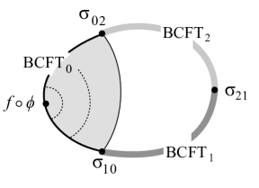
Figure 2.2: The BCC projector should structurally look like a surface of stretched string probed from a reference boundary conformal field theory. As shown above, such a surface should have an insertion of the boundary condition changing operator $\sigma_{21}$ between the BCFTs at the two endpoints. It should also have boundary condition changing operators $\sigma_{02}$ and $\sigma_{10}$ to probe with a test state.

Then an interpretation of the identity (2.31) immediately presents itself: $X^{\infty}$ is a star algebra projector representing a stretched string connecting the boundary conformal field theories of $\Phi_{2}$ and $\Phi_{1}$. To see this, suppose we represent a stretched string as a surface state with an insertion of a boundary condition changing operator $\sigma_{21}$ between the BCFTs of $\Phi_{2}$ and $\Phi_{1}$. In order to probe this surface with a test state, we need to insert two other BCC operators $\sigma_{02}$ and $\sigma_{10}$ on either side of $\sigma_{21}$ to match the boundary condition of the reference BCFT (See figure 2.2). Now if we compute the BRST variation of this object, we find a direct correspondence with the BRST variation of $X^{\infty}$: $\Phi_{2}$ corresponds to the the BRST variation of $\sigma_{02}$; $\Phi_{1}-\Phi_{2}$ corresponds to the BRST variation of $\sigma_{21}$; and $\Phi_{1}$ corresponds the BRST variation of $\sigma_{10}$ (See figure 2.3 A). The projector $X^{\infty}$ may not appear quite as simple as figure 2.2, since the way that string field theory represents worldsheet boundary conditions can be indirect. However, the shift in boundary condition inside $X^{\infty}$ is remarkably clear in the examples we have studied. Therefore, we call $X^{\infty}$ the boundary condition changing projector.

The identity (2.31) can be written in a few other forms which help illuminate the interpretation of $X^{\infty}$. For example,

$$Q_{\Phi_{2}\Phi_{1}}X^{\infty}=X^{\infty}(Q_{\Phi_{2}\Phi_{1}}1)X^{\infty}$$ (2.35)

is analogous to the statement that the BRST variation of a surface of stretched string only receives contribution from the boundary condition changing operator between the open string endpoints. (See figure 2.3 B). Multiplying (2.35) by $X^{\infty}$ on either side, we also find

$$(Q_{\Phi_{2}}X^{\infty})X^{\infty}=X^{\infty}(Q_{\Phi_{1}}X^{\infty})=0.$$ (2.36)

This corresponds to the statement that the boundary conditions are BRST invariant separately on each endpoint of the open string. (See figure 2.3 C).

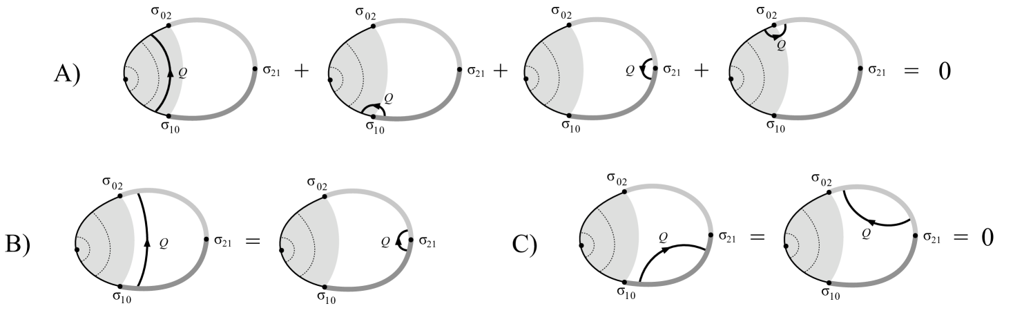
Figure 2.3: Figure A) demonstrates the analogy of equation (2.31), B) demonstrates the analogy of (2.35) and C) the analogy of (2.36).

When calculating the BRST variation of $X^{\infty}$ we assumed that all operators could be treated like finite dimensional matrices. However, in string field theory the double-projector term $X^{\infty}(\Phi_{1}-\Phi_{2})X^{\infty}$ in (2.31) is problematic, since star products of projector-like states are not in general well-defined. Therefore in string field theory equation (2.31) should be understood in the context of some regularization. Let us present two regularizations. The first represents the BCC projector as the limit

$$X^{\infty}=\lim_{\epsilon\to 0^{+}}\frac{\epsilon}{\epsilon+U}.$$ (2.37)

Assuming $U$ is a left gauge transformation from $\Phi_{1}$ to $\Phi_{2}$, we can easily calculate

$$Q\frac{\epsilon}{\epsilon+U}\!\!\!\!\!\!\!\! =-\frac{\epsilon}{\epsilon+U}QU\frac{1}{\epsilon+U}$$ (2.38)

$$=-\frac{\epsilon}{\epsilon+U}\Big{[}(U+\epsilon)\Phi_{2}-\Phi_{1}(U+\epsilon)+\epsilon(\Phi_{1}-\Phi_{2})\Big{]}\frac{1}{\epsilon+U}$$

$$=-\Phi_{2}\frac{\epsilon}{\epsilon+U}+\frac{\epsilon}{\epsilon+U}\Phi_{1}-\frac{\epsilon}{\epsilon+U}(\Phi_{1}-\Phi_{2})\frac{\epsilon}{\epsilon+U}.$$

Therefore

$$Q\frac{\epsilon}{\epsilon+U}+\Phi_{2}\frac{\epsilon}{\epsilon+U}+\frac{\epsilon}{\epsilon+U}(\Phi_{1}-\Phi_{2})\frac{\epsilon}{\epsilon+U}-\frac{\epsilon}{\epsilon+U}\Phi_{1}=0.$$ (2.39)

Note that this reproduces the basic form of (2.31) even before taking the $\epsilon\to 0$ limit. The second regularization represents the BCC projector as an infinite power of $X$:

$$X^{\infty}=\lim_{N\to\infty}X^{N}.$$ (2.40)

With some algebra one can prove the identity

$$QX^{2N}+\Phi_{2}X^{2N-1}+X^{N}(\Phi_{1}-\Phi_{2})X^{N}-X^{2N-1}\Phi_{1}=\mathcal{R}(N),$$ (2.41)

where the remainder $\mathcal{R}(N)$ is the expression

$$\mathcal{R}(N)\!\!\!\!\!\!\!\! =\left[\Phi_{1}X^{N-1}+X\sum_{k=0}^{N-2}X^{N-1-k}(\Phi_{1}-\Phi_{2})X^{k}\right]UX^{N}$$ (2.42)

$$\ \ \ +UX^{N}\left[-X^{N-1}\Phi_{2}+\sum_{k=0}^{N-2}X^{N-2-k}(\Phi_{1}-\Phi_{2})X^{k+1}\right].$$

Equation (2.41) reproduces (2.31) if $\mathcal{R}(N)$ vanishes in the $N\to\infty$ limit. The remainder does vanish if $X^{N}(\Phi_{1}-\Phi_{2})X^{N}$ is finite for large $N$.

2.4 BCC Projector vs. Characteristic Projector

Let us explain the relation between the BCC projector and the characteristic projector introduced by Ellwood [9]. The characteristic projector is defined given an arbitrary solution $\Phi$ together with a reference solution $\Psi$ and homotopy operator $A$ satisfying

$$Q_{\Psi}A=1,\ \ \ \ \ A^{2}=0.$$ (2.43)

This implies that the kinetic operator around $\Psi$ supports no cohomology, and therefore $\Psi$ can be interpreted as the tachyon vacuum [28, 30]. The characteristic projector is defined

$$P\equiv\lim_{N\to\infty}(-[A,\Phi-\Psi])^{N}.$$ (2.44)

We claim that the characteristic projector is the BCC projector for a singular gauge transformation from a solution to itself. To see this, note that

$$U_{1}\!\!\!\!\!\!\!\! =Q_{\Phi\Psi}A$$ (2.45)

$$=1+(\Phi-\Psi)A$$

is a left gauge transformation from $\Phi$ to the tachyon vacuum, and

$$U_{2}\!\!\!\!\!\!\!\! =Q_{\Psi\Phi}A$$ (2.46)

$$=1+A(\Phi-\Psi)$$

is a left gauge transformation from the tachyon vacuum to $\Phi$. Therefore the product,

$$U=U_{1}U_{2}=1+[A,\Phi-\Psi],$$ (2.47)

is a left gauge transformation from $\Phi$ to itself. To find the BCC projector we take the infinite power of

$$X=-[A,\Phi-\Psi].$$ (2.48)

This is just the characteristic projector. In [9] it was conjectured, and demonstrated in examples, that the characteristic projector is a sliver-like state representing the boundary conditions of $\Phi$ deep in its interior. The BCC projector should represent a change of boundary condition between two BCFTs. But in this case the source and target solutions are the same, so we only see the boundary conditions of a single BCFT, consistent with Ellwood’s interpretation of the characteristic projector.

One of the main insights of [9], which was an inspiration for the current work, was that singular gauge transformations could be thought of as possessing a kernel which could be described with a star algebra projector. However, the treatment of singular gauge transformations presented here differs substantially from [9]. A central assumption of [9], which we do not follow, is that the characteristic projector is annihilated by the homotopy operator:

$$AP=PA=0.$$ (2.49)

This equation is true in known examples in string field theory, provided one is only concerned with string fields as they are defined in the Fock space expansion. However, this assumption leads to a number of apparent inconsistencies. For example, the BCC projector for the left gauge transformation $U_{2}$ from the tachyon vacuum to $\Phi$ can be written

$$X^{\infty}=-PA(\Phi-\Psi)$$ (2.50)

Assuming (2.49) this means $X^{\infty}=0$, which implies that $U_{2}$ has no kernel and all solutions should be gauge equivalent to the tachyon vacuum. On the other hand, (2.49) also implies

$$U_{2}P=0$$ (2.51)

which contradicts what we just proved, i.e. that $U_{2}$ has no kernel. The contradiction comes because (2.49) implies an associativity anomaly [9]

$$P(U_{2}P)=0\neq P=(PU_{2})P$$ (2.52)

This means that (2.49) can never be true in the type of matrix-like model of the string field algebra we have been assuming. Therefore in our approach (2.49) is false, which means that we require a stronger notion of equality than the Fock space expansion of the string field. Indeed, we believe that this is physically necessary since (2.49) implies that the phantom term for Schnabl’s solution vanishes, which misses the nontrivial contribution the phantom term makes to gauge invariant observables. We will return to this issue in section 4.2.

2.5 Toy Model

Before considering string field theory, it is helpful to see how the formalism is supposed to work in a finite dimensional toy model. Suppose the open string star algebra is just the Clifford algebra generated by two elements $b,c$ satisfying

$$[b,c]=1,\ \ \ \ \ \ b^{2}=c^{2}=0.$$ (2.53)

These elements are Grassmann odd and have the obvious ghost number. The algebra allows a 2-dimensional representation $\mathcal{D}$ in terms of Pauli matrices. We define the BRST operator to be

$$Q=[c,\cdot].$$ (2.54)

The cohomology is empty. Therefore, our toy model can be thought of as a simplified version of vacuum string field theory [31].

The equation of motion,

$$Q\Phi+\Phi^{2}=0,$$ (2.55)

is easy to solve:

$$\Phi=-\lambda c,\ \ \ \ \lambda\in\mathbb{R}.$$ (2.56)

What is less obvious is whether any of these solutions is physically nontrivial. We can construct a left gauge transformation relating the tachyon vacuum $\Phi=0$ and the general solution $\Phi=-\lambda c$:

$$U\!\!\!\!\!\!\!\! =Q_{0,-\lambda c}b$$ (2.57)

$$=1-\lambda bc.$$

Computing the BCC projector with (2.14), we find:

$$X^{\infty}=\lim_{\epsilon\to 0}\left(\epsilon+\frac{\epsilon\lambda}{1-\lambda+\epsilon\lambda}bc\right).$$ (2.58)

The limit vanishes in all cases except $\lambda=1$, where the BCC projector becomes

$$X^{\infty}=bc,\ \ \ \ \ \ (\lambda=1).$$ (2.59)

Therefore our toy model has only one nontrivial solution:

$$\Phi=-c.$$ (2.60)

Note that the projector appears discontinuously at $\lambda=1$, and not in the $\lambda\to 1$ limit. This is reminiscent of how Schnabl’s solution formally appears to be a limit of pure gauge solutions as $\lambda\to 1$, but at $\lambda=1$ there is a physical discontinuity which brings the solution to the tachyon vacuum. A similar discontinuity appears for the pure gauge and tachyon vacuum solutions of Takahashi and Tanimoto [32, 33, 34]. In this toy model, what makes the solution $\Phi=-c$ different from the others is that it supports cohomology. In fact, the shifted kinetic operator vanishes identically:

$$Q-[c,\cdot]=0,$$ (2.61)

and therefore any nonzero state is in the cohomology. At ghost number 1 the cohomology includes only $c$, which we can interpret as the tachyon of an unstable brane. Therefore the solution $\Phi=-c$ represents a D-brane sitting on top of the tachyon vacuum.

Though the equations of motion are easy to solve in this model, let’s try to construct the solutions indirectly using singular gauge transformations. Within this subalgebra, there are only two nonzero and noninvertible ghost number zero fields which could give an interesting solution (up to a trivial multiplicative factor):

$$U_{1}\!\!\!\!\!\!\!\! =1-bc,\ \ \to\ \ X^{\infty}_{1}=bc,$$

$$U_{2}\!\!\!\!\!\!\!\! =1-cb,\ \ \to\ \ X_{2}^{\infty}=cb.$$ (2.62)

To the right of the arrow we wrote the corresponding BCC projector. Starting from the tachyon vacuum $\Phi=0$, the first case obviously corresponds to the solution $\Phi=-c$ which we have already discovered. What about the second case? It is easy to check that the weak consistency condition is not obeyed:

$$X_{2}^{\infty}QU_{2}=(cb)Q(1-cb)=c\neq 0,$$ (2.63)

so there is no corresponding solution. Now, given $U_{1}$, how do we reconstruct the solution $\Phi=-c$? Following (2.20), we need to define a formal inverse for $U_{1}$. It suffices to choose

$$(U_{1}^{-1})^{\prime}=1,$$ (2.64)

since this inverts $U_{1}$ up to the kernel of $U_{1}$. Then

$$\Phi\!\!\!\!\!\!\!\! =(U_{1}^{-1})^{\prime}QU_{1}+X_{1}^{\infty}\Phi^{\prime}$$ (2.65)

$$=Q(1-bc)+bc\Phi^{\prime}$$

$$=-c+bc\Phi^{\prime}.$$

Here we are lucky that any choice of $\Phi^{\prime}$ must be proportional to $c$, which is killed by $bc$. Therefore the phantom term vanishes and the solution is uniquely determined by $U_{1}$.

To see an example of a nontrivial phantom term, we have to consider a more complicated model. Suppose that the algebra consists of Clifford algebra generated by four elements $c_{1},c_{2},b_{1},b_{2}$ satisfying

$$[b_{i},c_{j}]=\delta_{ij},\ \ \ \ b_{i}^{2}=c_{i}^{2}=0\ \ \ \ \ \ \ \ \ (i,j=1,2).$$ (2.66)

with the obvious ghost number assignments. Taking $Q=[c_{1},\cdot]$, consider the solution

$$\Phi=-c_{1}+b_{1}c_{1}c_{2}.$$ (2.67)

This solution is nontrivial because the shifted kinetic operator supports cohomology. At ghost number 1 the cohomology is 1-dimensional and consists of states proportional to $c_{2}$ modulo exact terms:

$$Q_{\Phi}c_{2}=0,\ \ \ c_{2}\neq Q_{\Phi}(\mathrm{something}).$$ (2.68)

We can find a left gauge transformation from the tachyon vacuum to the solution (2.67):

$$U=Q_{0\Phi}b_{1}=1-b_{1}c_{1}.$$ (2.69)

The BCC projector is $X^{\infty}=b_{1}c_{1}$. Choosing $(U^{-1})^{\prime}=1$ we can reconstruct the solution out of $U$:

$$\Phi\!\!\!\!\!\!\!\! =(U^{-1})^{\prime}QU+X^{\infty}\Phi^{\prime}$$ (2.70)

$$=-c_{1}+X^{\infty}\Phi^{\prime}.$$

If we want the solution we started with, apparently we must have a nonzero phantom term:

$$X^{\infty}\Phi^{\prime}=(b_{1}c_{1})c_{2}.$$ (2.71)

Note that this choice requires additional information not contained in the left gauge transformation. In fact, we could have chosen the phantom term to vanish, though the resulting solution $\Phi=-c_{1}$ is physically different from the solution we started with. (The spectrum of fluctuations around $\Phi=-c_{1}$ includes all ghost number 1 states, not just $c_{2}$). As mentioned before, in string field theory the situation may be different, since regularity may fix the phantom term uniquely once we have chosen $U$.

3 The Category of Classical Solutions

It is interesting to ask what happens if we generalize the gauge group of open string field theory to include singular gauge transformations. Obviously we don’t have a group anymore since we don’t have inverses. But it is not even a semi-group, since the product of two left gauge transformations is not generally a left gauge transformation. However, it is a left gauge transformation if the target solution of the first left gauge transformation matches the source solution of the second. Let $U_{12}$ be a left gauge transformation from $\Phi_{1}$ to $\Phi_{2}$, and $U_{23}$ be a left gauge transformation from $\Phi_{2}$ to $\Phi_{3}$. Then the Leibniz rule (2.5) implies

$$Q_{\Phi_{1}\Phi_{3}}(U_{12}U_{23})=(Q_{\Phi_{1}\Phi_{2}}U_{12})U_{23}+U_{12}(Q_{\Phi_{2}\Phi_{3}}U_{23})=0,$$ (3.1)

so $U_{12}U_{23}$ is a left gauge transformation from $\Phi_{1}$ to $\Phi_{3}$. Therefore multiplication of left gauge transformations works like the composition of maps; we can only compose two maps if the image of the first is contained in the domain of the second.

The structure we’re describing is a category, which we call Left. The objects of Left are classical solutions, and the morphisms are left gauge transformations. Composition of morphisms is associative because the star product is associative. Each object has an identity morphism, which is just the identity string field $U=1$.

The category Left is a nice description of a structure, but we would like to get some insight into its physical meaning. To start, note that the operator $Q_{\Phi_{1}\Phi_{2}}$ is the kinetic operator for a stretched string in a $2\times 2$ string field theory expanded around the classical solution

$${\bf\Phi}=\left(\begin{matrix}\Phi_{1}&0\\ 0&\Phi_{2}\end{matrix}\right).$$ (3.2)

Then the morphisms of Left consist of ghost number zero states which are closed under the action of the kinetic operator of a stretched string. An important subset of these morphisms are those which are not only closed, but exact, i.e. take the form

$$U=Q_{\Phi_{1}\Phi_{2}}b.$$ (3.3)

We call these exact left gauge transformations. They form an ideal in Left, in the sense that the composition of any left gauge transformation with an exact left gauge transformation is again exact. As we will see, exact left gauge transformations are what make the category Left interesting.

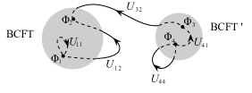
Figure 3.1: Schematic picture of the category Left. The points represent classical solutions, the curves represent left gauge transformations, and the grey circles enclose solutions describing the same BCFT. The curves inside the grey circles are proper gauge transformations, and those outside the circles are singular. Singular gauge transformations are often exact, and can be interpreted as generating surfaces of open string connecting BCFTs. Therefore the curves in this picture also represent open strings ending on D-branes.

Consider the exact left gauge transformation

$$K=QB,$$ (3.4)

which relates the perturbative vacuum to itself. The string field $K$ has an important property: It is a worldsheet Hamiltonian, and it generates a 1-parameter family of surfaces which define wedge states [8]:

$$\Omega^{t}=e^{-tK}.$$ (3.5)

In fact, this appears to be general: an exact left gauge transformations is a (generalized) BRST variation of an antighost, and therefore it is natural to think of it as generating a surface. If the “wedge state” $e^{-tU}$ converges in the $t\to\infty$ limit, we should get the BCC projector,

$$X^{\infty}=\lim_{t\to\infty}e^{-tU},$$ (3.6)

which, as we have conjectured, describes a surface of stretched string connecting two BCFTs. Therefore exact left gauge transformations have “endpoints” which are fixed to a source and target solution because open strings have endpoints fixed to corresponding D-branes. This gives a physical interpretation of the category Left: The objects, up to isomorphism, represent D-branes, and the morphisms represent open strings connecting them. (See figure 3.1). This structure is reminiscent of the description of D-branes in terms of derived categories [35, 36, 37], and it would be interesting to explore the relation.

One aspect of this picture requires explanation. Exact left gauge transformations are not necessarily singular, or vice-versa. Yet both should define a BCC projector with an open string interpretation. To explain the relation between exact and singular gauge transformations, we state two facts:

Fact 1.

The only exact left gauge transformations which are invertible relate the tachyon vacuum to itself.

Proof.

Suppose an exact left gauge transformation $U_{12}=Q_{\Phi_{1}\Phi_{2}}b$ has an inverse, $U_{12}^{-1}$. Then

$$1=U_{12}^{-1}U_{12}=Q_{\Phi_{2}\Phi_{2}}(U_{12}^{-1}b)=Q_{\Phi_{1}\Phi_{1}}(bU_{12}^{-1}).$$ (3.7)

This implies that both solutions $\Phi_{1}$ and $\Phi_{2}$ support no cohomology at any ghost number, so they must both describe the tachyon vacuum. ∎

This result is consistent with the expectation that exact left gauge transformations generate surfaces, and, at the same time, only singular gauge transformations define a nonzero BCC projector. The only case where an exact left gauge transformation can be nonsingular is around the tachyon vacuum, where there is no open string surface to generate.

Fact 2.

Any singular gauge transformation between two solutions is exact provided that the spectrum of stretched strings between the two corresponding backgrounds has no cohomology at ghost number $0$.

Proof.

This follows immediately from the assumption that the cohomology of $Q_{\Phi_{1}\Phi_{2}}$ should reproduce the cohomology of a stretched string connecting the BCFTs corresponding to the solutions $\Phi_{1}$ and $\Phi_{2}$. ∎

Generally, an open string connecting two D-branes will have different boundary conditions at its two endpoints, and therefore will have no cohomology at ghost number zero. So in the general situation, singular gauge transformations are exact. However, let us give two counterexamples. Consider a string field theory with $2\times 2$ Chan-Paton factors and two solutions

$${\bf\Phi}_{1}=0,\ \ \ \ \ \ \ \ \ {\bf\Phi}_{2}=\left(\begin{matrix}0&0\\ 0&\Phi\end{matrix}\right),$$ (3.8)

where $\Phi$ is a solution of the string field theory defined by the $2$-$2$ strings. Then

$${\bf U}=\left(\begin{matrix}1&0\\ 0&Q_{0\Phi}b\end{matrix}\right)$$ (3.9)

is a singular gauge transformation from ${\bf\Phi}_{1}$ to ${\bf\Phi}_{2}$ which is not exact, due to the identity string field in the $1$-$1$ component. The kernel of ${\bf U}$ is contained solely in the $2$-$2$ component, and the resulting BCC projector describes a single string stretching from the perturbative vacuum of the second D-brane to the background $\Phi$ of the second D-brane. There is no surface generated for strings attached to the first D-brane. To give a second example, consider the left gauge transformation

$$U=1-2\Omega,$$ (3.10)

which relates the perturbative vacuum to itself. The level expansion of $U$ starts with $-|0\rangle$, so it is not an exact left gauge transformation. However, the inverse $U^{-1}$ appears to be divergent, or at least it is not possible to express it as a superposition of wedge states [21, 38]. This problem can be understood from the fact that $U$, as a function of $K$, has a zero at $K=\ln 2$. The BCC projector of $U$ is formally

$$X^{\infty}(K)=\left\{\begin{matrix}1&\ \mathrm{for}\ K=\ln 2\\ 0&\ \mathrm{otherwise}\end{matrix}\right..$$ (3.11)

This projector can be considered as a limiting case of the class of infinite-rank projectors discussed in [21]. It vanishes in the Fock space, and it does not have a known representation in terms of open string surfaces. We do not know whether $U$ should be considered a singular gauge transformation in a physically important sense, or whether defining its inverse is just a technical problem.

4 Examples

In this section we demonstrate the weak consistency condition and the construction of the BCC projector for some known analytic solutions.

We will employ the algebraic notation for wedge states with insertions developed in [8, 39], following the conventions explained in appendix A of [20]. Let us review the essentials. We will frequently employ the string fields $K$ and $B$ introduced in [8], which correspond to vertical line integral insertions of the energy-momentum tensor and $b$-ghost in the cylinder coordinate system. We have $QB=K$, $[B,K]=0$, and $B^{2}=0$. Exponentials of $K$ define wedge states [40]:

$$\Omega^{t}=e^{-tK},$$ (4.1)

which are star algebra powers of the $SL(2,\mathbb{R})$ vacuum $\Omega\equiv|0\rangle$. The infinite power of the vacuum is a projector of the star algebra, the sliver state $\Omega^{\infty}$ [40, 41]. We will also encounter other string fields $c$, $\sigma_{10}$, and so on, which correspond to insertions of operators on the open string boundary in the cylinder coordinate system. For properties of these insertions we direct readers to the appropriate references where the solutions are described in detail.

4.1 Trivial case: $U=0$

The string field $U=0$ is a left gauge transformation between any two solutions. The associated BCC projector is the identity string field:

$$X^{\infty}=1.$$ (4.2)

We can interpret this as a projector where all boundary condition changing operators have collapsed on top of one another and canceled out. Both the strong and weak consistency conditions are satisfied. Using (2.20) we can therefore express $\Phi_{2}$ as a formal gauge transformation of $\Phi_{1}$:

$$\Phi_{2}=(0^{-1})^{\prime}(Q+\Phi_{1})0+1\cdot\Phi^{\prime}.$$ (4.3)

Since there are no nonzero vectors in the image of $U=0$, the operator $(0^{-1})^{\prime}$ must vanish over its entire domain. Then $\Phi_{2}=\Phi^{\prime}$, and the entire solution consists of the phantom term. Not surprisingly, $U=0$ does not give any information about how to construct $\Phi_{2}$ from $\Phi_{1}$.

4.2 Schnabl’s solution

Schnabl’s solution for the tachyon vacuum takes the form

$$\Psi=\sqrt{\Omega}c\frac{KB}{1-\Omega}c\sqrt{\Omega}.$$ (4.4)

As discovered by Okawa [8], Schnabl’s solution can be constructed as a left gauge transformation of the perturbative vacuum:

$$QU=U\Psi,$$ (4.5)

where

$$U=1-\sqrt{\Omega}cB\sqrt{\Omega}.$$ (4.6)

Now we want to compute the boundary condition changing projector and verify that Okawa’s $U$ satisfies the weak consistency condition. This will quickly lead to some puzzles, but with a few assumptions the formalism works consistently with our understanding of the physics.

The BCC projector is easy to compute from $U$:

$$X^{\infty}=\sqrt{\Omega}cB\Omega^{\infty}.$$ (4.7)

Since the field $B$ annihilates the sliver state in the Fock space, the BCC projector vanishes in the Fock space. But this means that Okawa’s $U$ should have an inverse! In fact, it is invertible in the Fock space:

$$U^{-1}=1-\sqrt{\Omega}cB\frac{1}{1-\Omega}\sqrt{\Omega},\ \ \ \ \ \ \ (\mathrm{formally}).$$ (4.8)

Expanding the factor $\frac{1}{1-\Omega}$ as a geometric series produces a linear divergence proportional to the sliver state, but this divergence is annihilated by $B$, so in total $U^{-1}$ is finite. This raises the obvious question: Why is Schnabl’s solution not pure gauge? The point is that it is not enough for $U$ to be invertible in the level expansion; it must be invertible from the perspective of the gauge invariant action, for example when contracting the solution with itself [8]. But in this context it is no longer true that $B$ annihilates the sliver state. This can be seen from the fact that the phantom term for Schnabl’s solution,

$$\lim_{N\to\infty}\psi_{N}=\sqrt{\Omega}cB\Omega^{\infty}c\sqrt{\Omega},$$ (4.9)

makes a nontrivial contribution to the energy [7]. Therefore, we must have

$$B\Omega^{\infty}\neq 0.$$ (4.10)

Under this assumption, the inverse of $U$ is divergent and the BCC projector is nonzero. Consistently, Schnabl’s solution is not pure gauge.

The above subtlety with $B\Omega^{\infty}$ may have a physical origin. Following the discussion of section 2.3, the BCC projector (4.7) should (in principle) represent an open string connecting the tachyon vacuum and the perturbative vacuum, as in figure 4.1. But there is no such open string; Any correlator with a boundary segment “attached” to the tachyon vacuum should vanish identically. Consistently, the BCC projector (4.7) vanishes in the Fock space. For other solutions we study, it will not vanish. Since the phantom term is proportional to the BCC projector, this also explains why the phantom term for Schnabl’s solution vanishes in the Fock space.

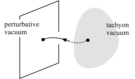
Figure 4.1: The BCC projector for Okawa’s left gauge transformation should describe a (hypothetical) open string with an endpoint disappearing into the tachyon vacuum.

Equation (4.10) implies that the BCC projector is nontrivial, but to apply the weak consistency condition we must also be able to assume that it is finite. This requires

$$K\Omega^{\infty}=0,$$ (4.11)

since, if the infinite power of the $SL(2,\mathbb{R})$ vacuum converges to a limit, we must have

$$\lim_{t\to\infty}\frac{d}{dt}\Omega^{t}=0.$$ (4.12)

The distinction between the string fields $B$ and $K$ with regard to the sliver state is subtle. We will proceed with the assumption (4.11) and see where it leads.

Let us give two simple examples which help illustrate the meaning of equations (4.10) and (4.11) for the purposes of the weak consistency condition. Consider the equation

$$B(1-\Omega)=KA,$$ (4.13)

which we want to solve for $A$. Since $K$ has a kernel, the solution may not exist. To check this, multiply by the equation by sliver state:

$$B\Omega^{\infty}(1-\Omega)=0.$$ (4.14)

The quantity $\Omega^{\infty}(1-\Omega)$ vanishes by (4.11), so the constraint is consistently satisfied. Indeed, the solution $A=B\frac{1-\Omega}{K}$ is the homotopy operator for Schnabl’s solution [28, 18], and is a well defined string field. Now, by contrast, consider the equation

$$B=KH,$$ (4.15)

which we want to solve for $H$. This time multiplying both sides by the sliver gives

$$B\Omega^{\infty}\stackrel{{\scriptstyle?}}{{=}}0,$$ (4.16)

which contradicts (4.10). Indeed, the formal solution $H=\frac{B}{K}$ does not exist, since otherwise $Q\frac{B}{K}=1$, which would trivialize the cohomology of physical states around the perturbative vacuum.

With this preparation, we can check the weak consistency condition for Okawa’s $U$.

$$X^{\infty}QU\!\!\!\!\!\!\!\! =\sqrt{\Omega}cB\Omega^{\infty}(cKBc\sqrt{\Omega})$$ (4.17)

$$=\sqrt{\Omega}cB(K\Omega^{\infty})c\sqrt{\Omega}$$

$$=0,$$

where in the last step we used (4.11). This result is consistent with the fact that Schnabl’s solution exists.

We can also consider a different left gauge transformation $\tilde{U}$ which maps (in the opposite direction) from Schnabl’s solution to the perturbative vacuum:

$$(Q+\Psi)\tilde{U}=\tilde{U}\cdot 0,$$ (4.18)

where

$$\tilde{U}=1-\sqrt{\Omega}Bc\sqrt{\Omega}.$$ (4.19)

The BCC projector is

$$\tilde{X}^{\infty}=\Omega^{\infty}Bc\sqrt{\Omega}.$$ (4.20)

To check the weak consistency condition, compute

$$Q_{\Psi}\tilde{U}=\sqrt{\Omega}\Big{(}c-[\Omega,c]\Big{)}\frac{KB}{1-\Omega}c\sqrt{\Omega}.$$ (4.21)

Then

$$\tilde{X}^{\infty}Q_{\Psi}\tilde{U}\!\!\!\!\!\!\!\! =\Omega^{\infty}Bc\Omega\Big{(}c-[\Omega,c]\Big{)}\frac{KB}{1-\Omega}c\sqrt{\Omega}$$ (4.22)

$$=\Omega^{\infty}(1-\Omega)[\Omega,c]\frac{KB}{1-\Omega}c\sqrt{\Omega}$$

$$=0,$$

consistently.

If we compose Okawa’s $U$ and $\tilde{U}$, we transform from the perturbative vacuum, to the tachyon vacuum, and back. The result is a singular gauge transformation from the perturbative vacuum to itself:

$$U_{0}=U\tilde{U}=1-\Omega.$$ (4.23)

The BCC projector of $U_{0}$ is the sliver state:

$$X_{0}^{\infty}=\Omega^{\infty}.$$ (4.24)

This also happens to be the characteristic projector computed in [9]. The sliver state can be seen as a surface of string connecting the perturbative vacuum to itself. Unlike the BCC projector for Okawa’s $U$, this does not vanish in the Fock space. However, let us explain a point of possible confusion: There are many left gauge transformations from the perturbative vacuum to itself whose BCC projector vanishes identically. The simplest example is $U=1$. What makes the BCC projector (4.24) nontrivial is that $U_{0}$ is an exact left gauge transformation,

$$U_{0}=Q\left(B\frac{1-\Omega}{K}\right),$$ (4.25)

and, as argued in section 3, exact left gauge transformations naturally generate a surface of string connecting the source and target BCFTs (which, in this case, happen to be the same). Proper gauge transformations, like $U=1$, should not really be viewed as open strings connecting solutions—indeed, a proper gauge transformation around one solution is also a proper gauge transformation around any other. Accordingly, they do not generate physically interesting BCC projectors.

4.3 Multibranes and Ghost Branes

Let see what the formalism has to say about the multiple brane and ghost brane solutions discussed in [11, 12]. These solutions are known to suffer from singularities related to their definition as formal gauge transformations of the perturbative vacuum [12, 14, 15].

The two-brane solution can be derived by applying Okawa’s $\tilde{U}$ in (4.19)—which takes the tachyon vacuum to the perturbative vacuum—once again to the perturbative vacuum [44] (see figure 4.2). The projector $\tilde{X}^{\infty}=\Omega^{\infty}Bc\sqrt{\Omega}$ is the same as before, but since we are starting from the perturbative vacuum, the weak consistency condition is different:

$$\tilde{X}^{\infty}Q\tilde{U}\!\!\!\!\!\!\!\! =-\Omega^{\infty}Bc\Omega cKBc\sqrt{\Omega}$$ (4.26)

$$=-\Omega^{\infty}c(1-\Omega)KBc\sqrt{\Omega}$$

$$=B\Omega^{\infty}cK(1-\Omega)c\sqrt{\Omega}.$$

This is not zero. This means that $\tilde{U}$ is not a consistent left gauge transformation applied to the perturbative vacuum, and there should be no corresponding 2-brane solution. Still the 2-brane solution can be formally defined, and recent studies have shown that it is possible to recover the correct tension from the action [11, 12, 15], the closed string tadpole [11, 12, 45], and, in a limiting case, the boundary state [14, 46]. This suggests that there is something essentially “correct” about the solution which remains to be understood.

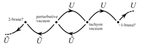
Figure 4.2: Multiple brane and ghost brane solutions can be formally defined by iterating the left gauge transformation $U$ from the perturbative vacuum to the tachyon vacuum, and the left gauge transformation $\tilde{U}$ from the tachyon vacuum to the perturbative vacuum.

Ghost brane solutions are defined by applying Okawa’s $U$ in (4.6) more than once to the perturbative vacuum [44]. They correspond to “removing” D-branes from an already empty vacuum (for a possible interpretation see [47]). For example, the $(-1)$-brane solution can be obtained by applying

$$U^{2}=1-\sqrt{\Omega}cB(2-\Omega)\sqrt{\Omega}$$ (4.27)

to the perturbative vacuum. We find the BCC projector is

$$X^{\infty}\!\!\!\!\!\!\!\! =\sqrt{\Omega}cB\left[\lim_{N\to\infty}\Omega^{N-1}(2-\Omega)^{N}\right]\sqrt{\Omega}$$ (4.28)

$$=\sqrt{\Omega}cB\Omega^{\infty},$$

which turns out to be the same BCC projector as for $U$ alone. To see whether $U^{2}$ is a sensible left gauge transformation, compute

$$X^{\infty}(QU^{2})\!\!\!\!\!\!\!\! =(X^{\infty}QU)U+(X^{\infty}U)QU$$ (4.29)

$$=0.$$

Surprisingly, the weak consistency condition does not reveal an obstruction for negative tension branes! Still, it turns out that $U^{2}$ is inconsistent. To see what’s going on, consider the equation

$$1-\Omega=K^{2}M.$$ (4.30)

which we want to solve for $M$. Multiplying both sides by the sliver state consistently gives $0=0$. But still (4.30) has no solution because the image of $K^{2}$ is smaller than the image of $1-\Omega$ (which vanishes only linearly at $K=0$). In a similar way, while $U^{2}$ satisfies the weak consistency condition, the BRST charge does not map the image of $U^{2}$ into itself.

Actually, there is nothing special going on here with the ghost brane solutions. It is a general expectation that the BCC projector for any left gauge transformation $U$ should be the same as for $U^{N}$ for any positive power $N$. Then it follows that the weak consistency condition is obeyed for any power $U^{N}$ if it is satisfied for $U$. For example, if we had applied Okawa’s $\tilde{U}$ twice to the tachyon vacuum, instead of once to the perturbative vacuum, the weak consistency condition would also work for the 2-brane solution. Therefore, to really test the ghost brane we should apply Okawa’s $U$ once to the tachyon vacuum, rather than twice to the perturbative vacuum. Then the weak consistency condition takes a different form:

$$X^{\infty}Q_{\Psi}U\!\!\!\!\!\!\!\! =X^{\infty}QU+X^{\infty}[\Psi,U]$$ (4.31)

$$=\sqrt{\Omega}cB\Omega^{\infty}\left(-c\frac{KB}{1-\Omega}c\Omega cB\sqrt{\Omega}+cB\Omega c\frac{KB}{1-\Omega}c\sqrt{\Omega}\right)$$

$$=\sqrt{\Omega}cB\Omega^{\infty}\left(-c\Omega cB\sqrt{\Omega}+c\sqrt{\Omega}\right)$$

$$=\sqrt{\Omega}cB\Omega^{\infty}c(2-\Omega)\sqrt{\Omega}.$$

This time we do not find zero.

It is interesting to speculate what the characteristic projector might look like for a 2-brane solution. Following the proposal of Ellwood [9], one expects that the characteristic projector of a solution $\Phi$ describes the boundary conditions of $\Phi$ towards the midpoint of the projector. We can generalize this proposal as follows. Let $U$ be a left gauge transformation from $\Phi_{1}$ to $\Phi_{2}$, and assume that $\Phi_{1}$ is real. Then the conjugate gauge parameter $U^{\ddagger}$ is a left gauge transformation from $\Phi_{2}^{\ddagger}$ to $\Phi_{1}$ and

$$U^{\ddagger}U$$ (4.32)

is a singular gauge transformation from $\Phi_{2}^{\ddagger}$ to $\Phi_{2}$. Assuming $\Phi_{2}^{\ddagger}$ and $\Phi_{2}$ are gauge equivalent, the BCC projector for $U^{\ddagger}U$ should describe the boundary conditions of the desired BCFT towards the midpoint. For multiple brane solutions, these boundary conditions must include Chan-Paton factors, and it has been speculated that the Chan-Paton structure should be described by higher rank star algebra projectors [9, 22, 41, 48]. On the other hand, applying this argument to the formal 2-brane solution constructed from Okawa’s $\tilde{U}$ gives

$$\tilde{U}^{\ddagger}\tilde{U}=1-\Omega$$ (4.33)

whose BCC projector is the sliver state. The sliver state is believed to be (in some sense) a rank one projector, so we would not expect this ansatz to reproduce the non-abelian Chan-Paton structure of the 2-brane.

4.4 Ellwood/BMT Lumps

Following [9], there has been interest in using singular gauge transformations to construct solutions describing the endpoint of an RG flow triggered by a relevant deformation [10, 13, 49], which in particular can describe the tachyon lump [50]. A simple example of such a solution was discovered by Bonora, Tolla and one of the authors (BMT) and takes the form [10]

$$\Phi=c\phi-\frac{B}{K+\phi}\phi^{\prime}c\partial c,$$ (4.34)

where $\phi$ is a relevant matter operator in the reference boundary conformal field theory and $\phi^{\prime}$ describes the failure of $\phi$ to be marginal. The operator $\phi$ must be appropriately “tuned” to trigger an RG flow to the desired boundary conformal field theory ($\mathrm{BCFT}^{*}$) in the infrared [9, 10, 13].

The solution can be derived from the tachyon vacuum [20]

$$\Psi=\frac{1}{1+K}(c+Q(Bc)),$$ (4.35)

using a (naive) singular gauge transformation [10]

$$U=1-\frac{1}{1+K}(1-\phi)Bc.$$ (4.36)

To derive the BCC projector, we use the formula (2.14) (with a redefinition $\epsilon\to\epsilon/\bar{\epsilon}$):

$$X^{\infty}=\lim_{\epsilon\to 0^{+}}\frac{\epsilon}{\epsilon+\bar{\epsilon}U},\ \ \ \ \ \ \ \bar{\epsilon}\equiv 1-\epsilon.$$ (4.37)

This gives

$$X^{\infty}\!\!\!\!\!\!\!\! =\lim_{\epsilon\to 0^{+}}\left[\frac{\epsilon}{1-\frac{\bar{\epsilon}}{1+K}(1-\phi)Bc}\right]$$ (4.38)

$$=\lim_{\epsilon\to 0^{+}}\left[\epsilon+\frac{\epsilon}{1-\frac{\bar{\epsilon}}{1+K}(1-\phi)}\frac{\bar{\epsilon}}{1+K}(1-\phi)Bc\right]$$

$$=\lim_{\epsilon\to 0^{+}}\left[\frac{\epsilon}{\epsilon+K+\bar{\epsilon}\phi}\right](1-\phi)Bc.$$

As shown in [13], the limit in parentheses converges to the so-called deformed sliver state $\tilde{\Omega}^{\infty}$, which is the sliver state with an insertion of the relevant boundary interaction at constant RG coupling in the upper half plane representation. Then the BCC projector is

$$X^{\infty}=\tilde{\Omega}^{\infty}(1-\phi)Bc.$$ (4.39)

This state vanishes in the Fock space, which is apparently a consequence of the fact that the source solution is the tachyon vacuum.

If we map the deformed sliver state to the unit disk representation [41], the midpoint of the local coordinate touches the boundary of the disk, splitting the surface in two. Since the conformal transformation is singular at the midpoint, the RG coupling of the relevant boundary interaction is pushed to the strict infrared, so that the disk correlator has $\mathrm{BCFT}^{*}$ boundary conditions precisely where the midpoint of the local coordinate touches the boundary of the unit disk. In this sense, the BCC projector (4.39) has $\mathrm{BCFT}^{*}$ boundary conditions at the midpoint. In fact, the naive left gauge transformation (4.36) was constructed to give precisely this result, based on the conjecture of Ellwood [9] that the characteristic projector of a solution $\Phi$ should have boundary conditions corresponding to the BCFT of $\Phi$ at the midpoint. While this idea seems correct, it is not sufficient; The BRST variation of $U$ must be proportional to $U$.

To see if this is the case, let’s look at the weak consistency condition. We assume (4.10) and the analogue of (4.11) for the deformed sliver state:

$$(K+\phi)\tilde{\Omega}^{\infty}=0.$$ (4.40)

Computing

$$Q_{\Psi}U=-(1-\phi)c+\frac{1}{1+K}(K+\phi)\frac{1}{1+K}Bc\partial c-\frac{B}{1+K}\phi^{\prime}c\partial c,$$ (4.41)

we find

$$X^{\infty}Q_{\Psi}U=-\tilde{\Omega}^{\infty}(1-\phi)\frac{1}{1+K}\left[(K+\phi)\frac{1}{1+K}Bc\partial c-B\phi^{\prime}c\partial c\right].$$ (4.42)

Now use (4.40) to replace $1-\phi$ with $1+K$. Then there is a cancellation with $\frac{1}{K+1}$ and the first term in brackets disappears when $K+\phi$ hits the deformed sliver. This leaves

$$X^{\infty}Q_{\Psi}U=-\tilde{\Omega}^{\infty}B\phi^{\prime}c\partial c.$$ (4.43)

The operator $\phi^{\prime}$ does not generally annihilate the deformed sliver [13], so the weak consistency condition is violated. The only way to avoid this problem is to set $\phi^{\prime}=0$, in which case the BMT solution describes a marginal deformation, or to set $\tilde{\Omega}^{\infty}=0$ in which case the BMT solution describes the tachyon vacuum. Otherwise, the BMT solution is singular and does not satisfy the equations of motion [13]. Nevertheless, the solution is (in a sense) very close to solving the equations of motion, and if one carefully treats its singularities, one can recover almost all of the expected physics of the RG flow [13, 49].

4.5 Solutions of Kiermaier, Okawa, and Soler

To see a shift in boundary condition inside the BCC projector, we should consider a singular gauge transformation relating two solutions which describe distinct backgrounds which support open string states. For this purpose, it is useful to study the solutions discovered by Kiermaier, Okawa, and Soler [29] (the KOS solutions):

$$\Phi=-(c\partial\sigma_{01})\frac{1}{1+K}\sigma_{10}(1+K)Bc\frac{1}{1+K}.$$ (4.44)

Here $\sigma_{01}$ and $\sigma_{10}$ are dimension $0$ primaries with the property that $\sigma_{01}\sigma_{10}=1$. In interesting examples, $\sigma_{01}$ and $\sigma_{10}$ are boundary condition changing operators from a reference $\mathrm{BCFT}_{0}$ to the open string background $\mathrm{BCFT}_{1}$ described by the solution. Under these assumptions the KOS solution is known to describe nonsingular marginal deformations [29, 51].

We can build the KOS solution with a left gauge transformation out of the tachyon vacuum:

$$U\!\!\!\!\!\!\!\! =Q_{\Psi\Phi}\left(\frac{B}{1+K}\right)$$ (4.45)

$$=1-\sigma_{01}\frac{1}{1+K}\sigma_{10}(1+K)Bc\frac{1}{1+K},$$

where we choose $\Psi$ to be the “simple” tachyon vacuum solution [20]:

$$\Psi=(c+Q(Bc))\frac{1}{1+K}.$$ (4.46)

Computing the BCC projector we find

$$X^{\infty}=\sigma_{01}\Omega^{\infty}\sigma_{10}(1+K)Bc\frac{1}{1+K}.$$ (4.47)

As expected, this vanishes in the Fock space since there are no open strings connecting the tachyon vacuum to the marginally deformed D-brane. To check the weak consistency condition, compute

$$Q_{\Psi}U=\left(c(1+K)\sigma_{01}\frac{1}{1+K}\sigma_{10}+\sigma_{01}\left[c,\frac{1}{1+K}\right]\sigma_{10}\right)(1+K)Bc\frac{1}{1+K},$$ (4.48)

and then multiply by the BCC projector:

$$X^{\infty}Q_{\Psi}U\!\!\!\!\!\!\!\! =\left(\sigma_{01}\Omega^{\infty}B\partial c\frac{1}{1+K}\sigma_{10}-\sigma_{01}\Omega^{\infty}B\left[c,\frac{1}{1+K}\right]\sigma_{10}\right)(1+K)c\frac{1}{1+K}$$ (4.49)

$$=\left(\sigma_{01}\Omega^{\infty}Bc\frac{1}{1+K}\sigma_{10}-\sigma_{01}\Omega^{\infty}Bc\sigma_{10}\right.$$

$$\ \ \ \ \ \ \left.-\sigma_{01}\Omega^{\infty}Bc\frac{1}{1+K}\sigma_{10}+\sigma_{01}\Omega^{\infty}Bc\sigma_{10}\right)(1+K)c\frac{1}{1+K}$$

$$=0,$$

where in the second step we wrote $\partial c=[1+K,c]$ and canceled $K$ against the sliver. If we had only guessed the left gauge transformation (4.45) without knowing about the KOS solution from the beginning, the final cancellation in (4.49) would seem quite miraculous. For example, suppose we tried to build a marginal solution like KOS from the tachyon vacuum using

$$U\stackrel{{\scriptstyle?}}{{=}}1-\sigma_{01}\frac{1}{1+K}\sigma_{10}Bc.$$ (4.50)

At first sight, this guess seems physically plausible. It is non invertible, and the BCC projector vanishes in the Fock space and has $\mathrm{BCFT}_{1}$ boundary conditions at the midpoint. Nevertheless, this ansatz fails to satisfy the weak consistency condition. This is an important point: Constructing new solutions by a pure gauge ansatz requires more than a plausible guess. The structure of the ansatz has to work in a nontrivial fashion.

Our main interest in this section is computing a boundary condition changing projector which displays a shift in boundary condition between two nontrivial backgrounds. Accordingly, consider two KOS solutions:

$$\Phi_{1}\!\!\!\!\!\!\!\! =-(c\partial\sigma_{01})\frac{1}{1+K}\sigma_{10}(1+K)Bc\frac{1}{1+K},\ \ \ \ \ \ \ \ (\mathrm{BCFT}_{1}),$$

$$\Phi_{2}\!\!\!\!\!\!\!\! =-(c\partial\sigma_{02})\frac{1}{1+K}\sigma_{20}(1+K)Bc\frac{1}{1+K},\ \ \ \ \ \ \ \ (\mathrm{BCFT}_{2}).$$ (4.51)

related by the left gauge transformation

$$U_{12}\!\!\!\!\!\!\!\! =Q_{\Phi_{1}\Phi_{2}}\left(\frac{B}{1+K}\right)$$ (4.52)

$$=1-cB(1+K)\sigma_{01}\frac{1}{1+K}\sigma_{10}\frac{1}{1+K}-\sigma_{02}\frac{1}{1+K}\sigma_{20}(1+K)Bc\frac{1}{1+K}.$$

Note that $U_{12}$ can be factorized into a product of left gauge transformations passing through the tachyon vacuum (4.46). The reason is the following: If $A$ is a homotopy operator of a tachyon vacuum solution $\Psi$, and $A^{2}=0$, we can factorize any exact left gauge transformation derived from $A$ into a product of two left gauge transformations passing through $\Psi$:

$$Q_{\Phi_{1}\Phi_{2}}A=(Q_{\Phi_{1}\Psi}A)(Q_{\Psi\Phi_{2}}A).$$ (4.53)

We do not believe this property is essential for the interpretation of the BCC projector, but it would be worth understanding this issue.

To compute the BCC projector we use (4.37)

$$X_{12}^{\infty}=\lim_{\epsilon\to 0^{+}}\frac{\epsilon}{\epsilon+\bar{\epsilon}U_{12}}.$$ (4.54)

Plugging in $U_{12}$,

$$\frac{\epsilon}{\epsilon+\bar{\epsilon}U_{12}}\!\!\!\!\!\!\!\! =\frac{\epsilon}{1-\bar{\epsilon}\left[cB(1+K)\sigma_{01}\frac{1}{1+K}\sigma_{10}+\sigma_{02}\frac{1}{1+K}\sigma_{20}(1+K)Bc\right]\frac{1}{1+K}}$$

$$=\frac{\epsilon}{\left(1-\bar{\epsilon}cB(1+K)\sigma_{01}\frac{1}{1+K}\sigma_{10}\frac{1}{K+1}\right)\left(1-\bar{\epsilon}\sigma_{02}\frac{1}{1+K}\sigma_{20}(1+K)Bc\frac{1}{1+K}\right)}$$

$$=\epsilon\left(\frac{1}{1-\bar{\epsilon}\sigma_{02}\frac{1}{1+K}\sigma_{20}(1+K)Bc\frac{1}{1+K}}\right)\left(\frac{1}{1-\bar{\epsilon}cB(1+K)\sigma_{01}\frac{1}{1+K}\sigma_{10}\frac{1}{K+1}}\right)$$

$$=\epsilon\left(1+\sigma_{02}\frac{\bar{\epsilon}}{K+\epsilon}\sigma_{20}(1+K)Bc\frac{1}{1+K}\right)\left(1+cB(1+K)\sigma_{01}\frac{\bar{\epsilon}}{\epsilon+K}\sigma_{10}\frac{1}{1+K}\right).$$

At this point we can already see the boundary conditions of $\mathrm{BCFT}_{2}$ gathering on the left and the boundary conditions of $\mathrm{BCFT}_{1}$ on the right. Multiplying this out we get four terms:

$$\frac{\epsilon}{\epsilon+\bar{\epsilon}U_{12}}\!\!\!\!\!\!\!\! =\epsilon+\bar{\epsilon}\left(\sigma_{02}\frac{\epsilon}{\epsilon+K}\sigma_{20}(1+K)Bc\frac{1}{1+K}\right)+\bar{\epsilon}\left(cB(1+K)\sigma_{01}\frac{\epsilon}{\epsilon+K}\sigma_{10}\frac{1}{1+K}\right)$$ (4.56)

$$\ \ \ \ \ +\bar{\epsilon}^{2}\left(\sigma_{02}\frac{\epsilon}{\epsilon+K}\sigma_{21}B\partial c\frac{1}{\epsilon+K}\sigma_{10}\frac{1}{1+K}\right),$$

where $\sigma_{21}\equiv\sigma_{20}\sigma_{01}$ is the boundary condition changing operator between $\mathrm{BCFT}_{2}$ and $\mathrm{BCFT}_{1}$. For simplicity we are assuming that $\sigma_{20}$ and $\sigma_{01}$ have trivial contractions. In principle this assumption should not be necessary—the collision between $\sigma_{20}$ and $\sigma_{01}$ could be vanishing or divergent, depending on whether the BCC operator $\sigma_{21}$ has positive or negative conformal dimension. However, this limitation is an artifact of the KOS solution and the chosen left gauge transformation (4.52). Other choices naturally regulate the collision. But we are seeing a precursor to a deeper issue that we will discuss shortly.

To simplify (4.56) further, consider the fourth term and expand using the Schwinger parameterization:

$$\frac{1}{\epsilon+K}{\sigma_{21}B\partial c}\frac{1}{\epsilon+K}=\int_{0}^{\infty}dt\,e^{-\epsilon t}\int_{0}^{t}ds\,\Omega^{t-s}\sigma_{21}B\partial c\Omega^{s}.$$ (4.57)

Note the identity

$$\partial\left(\int_{0}^{t}ds\,\Omega^{t-s}\Phi\Omega^{s}\right)=[\Phi,\Omega^{t}].$$ (4.58)

This suggests that we define the formal expression

$$\frac{1}{\partial}[\Phi,\Omega^{t}]\equiv\int_{0}^{t}\Omega^{t-s}\Phi\Omega^{s}.$$ (4.59)

Then we can write

$$\frac{1}{\epsilon+K}{\sigma_{21}B\partial c}\frac{1}{\epsilon+K}=\frac{1}{\partial}\left[\sigma_{21}B\partial c,\frac{1}{\epsilon+K}\right],$$ (4.60)

and (4.56) becomes

$$\frac{\epsilon}{\epsilon+\bar{\epsilon}U_{12}}\!\!\!\!\!\!\!\! =\epsilon+\bar{\epsilon}\left(\sigma_{02}\frac{\epsilon}{\epsilon+K}\sigma_{20}(1+K)Bc\frac{1}{1+K}\right)+\bar{\epsilon}\left(cB(1+K)\sigma_{01}\frac{\epsilon}{\epsilon+K}\sigma_{10}\frac{1}{1+K}\right)$$ (4.61)

$$\ \ \ \ \ +\bar{\epsilon}^{2}\left(\sigma_{02}\frac{1}{\partial}\left[\sigma_{21}B\partial c,\frac{\epsilon}{\epsilon+K}\right]\sigma_{10}\frac{1}{1+K}\right).$$

Finally, taking the $\epsilon\to 0^{+}$ limit gives:

$$\!\!\!\!\!\!\!\!\!\!\!\!\!\!\!\!\!\!\!\!\!\!X_{12}^{\infty}\!\!\!\!\!\!\!\! =\Bigg{[}\Big{(}cB(1+K)\,\sigma_{01}\Omega^{\infty}\sigma_{10}\Big{)}+\Big{(}\sigma_{02}\Omega^{\infty}\sigma_{20}\,(1+K)Bc\Big{)}$$ (4.62)

$$\ \ \ \ \ \ \ \ \ \ \ \ \ \ \ \ \ \ \ \ \ \ \ \ \ \ \ \ \ \ \ \ \ \ \ \ \ \ \ \ +\Big{(}\sigma_{02}\,\frac{1}{\partial}\big{[}\sigma_{21}B\partial c,\Omega^{\infty}\big{]}\sigma_{10}\Big{)}\Bigg{]}\frac{1}{1+K}.$$

The first two terms are BCC projectors for left gauge transformations from $\Phi_{1}$ to the tachyon vacuum (4.46), and from the tachyon vacuum to $\Phi_{2}$. These terms vanish in the Fock space. The last term contains a shift in boundary condition between $\mathrm{BCFT}_{2}$ and $\mathrm{BCFT}_{1}$, which is integrated (with some ghosts) through the entire width of the sliver state (see figure 4.3). This term does not vanish in the Fock space.

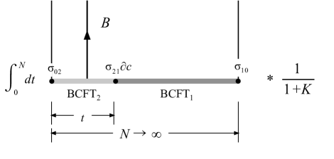
Figure 4.3: Cylinder representation of the nontrivial term in the BCC projector (4.62). The integration over $t$ moves the boundary condition changing operator over the whole width of the sliver state.

The BCC projector we just computed should reduce to the characteristic projector in the special case when $\mathrm{BCFT}_{2}=\mathrm{BCFT}_{1}$. Let’s see how this happens:

$$X_{11}^{\infty}\!\!\!\!\!\!\!\! =\left[cB(1+K)\sigma_{01}\Omega^{\infty}\sigma_{10}+\sigma_{01}\Omega^{\infty}\sigma_{10}(1+K)Bc+\sigma_{01}\frac{1}{\partial}\partial[Bc,\Omega^{\infty}]\sigma_{10}\right]\frac{1}{1+K}$$ (4.63)

$$=\Big{[}cB(1+K)\sigma_{01}\Omega^{\infty}\sigma_{10}+\sigma_{01}\Omega^{\infty}\sigma_{10}(1+K)Bc+Bc\sigma_{01}\Omega^{\infty}\sigma_{10}-\sigma_{01}\Omega^{\infty}\sigma_{10}Bc\Big{]}\frac{1}{1+K}$$

$$=\sigma_{01}\Omega^{\infty}\sigma_{10}\frac{1}{1+K}+\Big{[}cBK\sigma_{01}\Omega^{\infty}\sigma_{10}+\sigma_{01}\Omega^{\infty}\sigma_{10}KBc\Big{]}\frac{1}{1+K}.$$

Since $K$ annihilates the sliver, the $K$s next to the BCC operators in the second term can be traded with worldsheet derivatives. Then

$$X_{11}^{\infty}=\sigma_{01}\Omega^{\infty}\sigma_{10}\frac{1}{1+K}+\Big{[}(Q\sigma_{01})B\Omega^{\infty}\sigma_{10}-\sigma_{01}B\Omega^{\infty}(Q\sigma_{10})\Big{]}\frac{1}{1+K},$$ (4.64)

and the characteristic projector simplifies to

$$X_{11}^{\infty}=\Bigg{[}\sigma_{01}\Omega^{\infty}\sigma_{10}+Q\Big{(}\sigma_{01}B\Omega^{\infty}\sigma_{10}\Big{)}\Bigg{]}\frac{1}{1+K}.$$ (4.65)

Extrapolating from Schnabl gauge, this expression agrees with the characteristic projector computed in [9] except for the second term, which would have been ignored in [9] because it vanishes in the Fock space. Further specifying $\mathrm{BCFT}_{1}=\mathrm{BCFT}_{0}$ gives $X_{00}^{\infty}=\Omega^{\infty}$, which is the BCC projector for a singular gauge transformation from the perturbative vacuum to itself.

The form of the BCC projector $X_{12}^{\infty}$ substantially simplifies if we only contract with regular test states. Then first two terms in (4.62) can be ignored, and the third term simplifies to:

$$X_{12}^{\infty}=\Big{[}\sigma_{02}\Omega^{\infty}\sigma_{21}\Omega^{\infty}\sigma_{10}\Big{]}\frac{1}{1+K},\ \ \ \ \ \ (\mathrm{Fock\ space}).$$ (4.66)

For the detailed argument, see appendix A. This is precisely the structure we expected: $X_{12}^{\infty}$ is proportional to the sliver state with the boundary conditions of $\mathrm{BCFT}_{2}$ on its left half and the boundary conditions of $\mathrm{BCFT}_{1}$ on its right half, with the BCC operator $\sigma_{21}$ inserted at the midpoint (see figure 4.4).

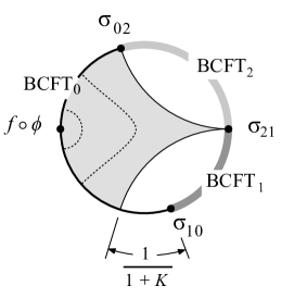
Figure 4.4: The BCC projector (4.62) contracted with a Fock space state, represented as a correlator on the unit disk. Note that the change of boundary condition happens precisely at the point where the midpoint of the local coordinate touches the boundary of the disk.

The KOS solutions are a special case of the solutions for regular marginal deformations in dressed Schnabl-gauges [20, 52]. Let us see how this discussion extends to the Schnabl-gauge marginal solutions [53, 54]:

$$\Phi_{1}\!\!\!\!\!\!\!\! =\sqrt{\Omega}\,cV_{1}\frac{1}{1+\frac{1-\Omega}{K}V_{1}}Bc\,\sqrt{\Omega},\ \ \ \ \ \ \ \ \ \ \ (\mathrm{BCFT}_{1}),$$

$$\Phi_{2}\!\!\!\!\!\!\!\! =\sqrt{\Omega}\,cV_{2}\frac{1}{1+\frac{1-\Omega}{K}V_{2}}Bc\,\sqrt{\Omega},\ \ \ \ \ \ \ \ \ \ \ (\mathrm{BCFT}_{2}),$$ (4.67)

where $V_{1},V_{2}$ are nonsingular marginal currents. These solutions can be related by a left gauge transformation

$$U_{12}\!\!\!\!\!\!\!\! =Q_{\Phi_{1}\Phi_{2}}\left(B\frac{1-\Omega}{K}\right)$$ (4.68)

$$=1-\sqrt{\Omega}\,cB\frac{1}{1+V_{1}\frac{1-\Omega}{K}}\,\sqrt{\Omega}-\sqrt{\Omega}\frac{1}{1+\frac{1-\Omega}{K}V_{2}}Bc\,\sqrt{\Omega}.$$

This left gauge transformation factorizes through Schnabl’s solution for the tachyon vacuum, (4.4). Computing the BCC projector, we find three terms analogous to (4.62):

$$X_{12}^{\infty}\!\!\!\!\!\!\!\! \ =\ \sqrt{\Omega}\Bigg{[}\left(cB\frac{K}{1-\Omega}\sigma_{01}\Omega^{\infty}\sigma_{10}\right)+\left(\sigma_{02}\Omega^{\infty}\sigma_{20}\frac{K}{1-\Omega}Bc\right)$$ (4.69)

$$\ \ \ \ \ \ \ \ \ \ \ \ \ \ \ \ \ \ \ \ \ +\left(\sigma_{02}\frac{1}{\partial}\left[\sigma_{20}\frac{K}{1-\Omega}Bc\Omega cB\frac{K}{1-\Omega}\sigma_{01},\Omega^{\infty}\right]\sigma_{10}\right)\Bigg{]}\sqrt{\Omega}.$$

The first two terms are BCC projectors for singular gauge transformations from $\Phi_{1}$ to the tachyon vacuum and from the tachyon vacuum to $\Phi_{2}$. In the third term, note that $\sigma_{20}$ and $\sigma_{01}$ are separated by a finite region of undeformed surface,

$$\sigma_{20}\frac{K}{1-\Omega}Bc\Omega cB\frac{K}{1-\Omega}\sigma_{01},$$ (4.70)

unlike with KOS, where they collide to form $\sigma_{21}$. However, in the projector limit the collision between $\sigma_{10}$ and $\sigma_{02}$ effectively re-emerges since the surface separating them is squeezed to vanishing width at the midpoint:

$$X_{12}^{\infty}=\sqrt{\Omega}\,\sigma_{02}\Omega^{\infty}\sigma_{21}\Omega^{\infty}\sigma_{10}\,\sqrt{\Omega},\ \ \ \ \ \ (\mathrm{Fock\ space}).$$ (4.71)

Now if $\sigma_{21}$ has nonzero conformal dimension, the BCC projector will be vanishing or infinite in the Fock space as a result of the singular conformal transformation of $\sigma_{21}$. This problem is most likely generic. Between any pair of BCFTs, the boundary condition changing operator generally carries nonzero conformal weight, and if the BCC projector places this operator at the midpoint, there will be a vanishing or divergent factor when contracting with Fock space states.

This problem should be irrelevant if we are using the BCC projector inside the phantom term to compute physical observables [55]. Still we would like to see the BCC projector shift the boundary condition in a nonsingular fashion when contracted with regular test states. One way around this problem is to put the operator $\sigma_{21}$ on-shell, that is, replace $\sigma_{21}\to c\mathcal{V}_{21}$, where $c\mathcal{V}_{21}$ is a dimension zero element of the cohomology of $Q$ for a stretched string between the BCFTs of $\Phi_{2}$ and $\Phi_{1}$. Then the “on-shell” BCC projector takes the form

$$X_{\mathcal{V}_{21}}^{\infty}=\sqrt{\Omega}\,\sigma_{20}\Omega^{\infty}\,c\mathcal{V}_{21}\,\Omega^{\infty}\sigma_{10}\,\sqrt{\Omega}.$$ (4.72)

This is now a nonsingular state in the Fock space, and is a projector-like representative of the ghost number 1 cohomology of $Q_{\Phi_{1}\Phi_{2}}$. In a much more physical sense than the bare BCC projector, $X^{\infty}_{\mathcal{V}_{12}}$ represents a stretched string connecting two BCFTs. Note that BCC projectors around the tachyon vacuum cannot be made nonvanishing in this way, since there are no on-shell states to insert at the midpoint. One shortcoming of this picture is that we would like to define the on-shell BCC projector as a limit of a sequence of regular states, rather than by hand after the projector limit has been taken. We will leave this problem to future work.

5 Summary and Discussion

The results of this paper can be summarized by three central ideas:

1) Any two classical solutions in open string field theory can be related by a left gauge transformation, i.e. formal gauge transformation defined by a finite gauge parameter $U$ possibly without an inverse. Left gauge transformations define the morphisms of a category Left, whose objects are classical solutions.

2) Given any left gauge transformation connecting solutions $\Phi_{1}$ and $\Phi_{2}$, one can define a star algebra projector which describes a stretched string connecting the BCFTs of $\Phi_{1}$ and $\Phi_{2}$. We call this the boundary condition changing projector. The boundary condition changing projector allows us to naturally associate the morphisms of Left with open strings connecting D-branes. It also determines the nontrivial part of the mysterious phantom term, as will be described in subsequent work [55].

3) Given any left gauge transformation $U$ from a source solution $\Phi_{1}$ to any target solution $\Phi_{2}$, the kinetic operator around $\Phi_{1}$ maps the image of $U$ into itself. This observation can be used to constrain the possible $U$s which define consistent left gauge transformations, as summarized by the strong and weak consistency conditions, (2.8) and (2.16). If one wants to construct a new solution using singular gauge transformations, one must be sure that the proposed $U$ satisfies these consistency conditions.

We have tried to provide a clear account of these ideas and their motivation, though there are many aspects of this picture which remain unexplored and we hope can be clarified in future work. Our understanding of the BCC projector, in particular, is preliminary. It would be desirable to extend our analysis to more examples, especially for solutions describing singular marginal deformations [3, 4, 5, 6]. Some aspects of these ideas could in principle be tested in the level expansion. For example, one could construct (numerically) a singular gauge transformation from the perturbative vacuum to the Siegel gauge tachyon condensate [56, 57, 58, 59], and verify that its BCC projector tends to vanish in the level expansion, but still nontrivially computes the shift in the closed string tadpole amplitude between the perturbative vacuum and the tachyon vacuum (via the Siegel gauge analogue of the phantom term for Schnabl’s solution).

A central assumption of our work is that the image and kernel of a left gauge transformation are linearly independent and span the whole space, and therefore define a boundary condition changing projector. However, it is not difficult to find ghost number zero string fields where this assumption is false, for example

$$U=B\partial c$$ (5.1)

This is nilpotent, so its kernel and image are not linearly independent. However, we are not aware of any genuine left gauge transformations of this type. That does not mean they do not exist, and do not have an important role to play in the construction of classical solutions. A particularly interesting possibility is that solutions could be constructed with left gauge transformations that are non-unitary isometries [26, 27].

It would be interesting to see if our results have some generalization to other string field theories, especially nonpolynomial superstring field theory [60, 61] and open string field theories based on homotopy associative algebras [62]. It is even possible that these ideas have some realization in closed string field theory [63], but the analogy between left gauge transformations and open strings suggests that a different type of structure might be needed there. It would also be interesting to see if left gauge transformations can be related to the derived category of the topological B-model [35, 36, 37]. If so, the category Left could provide a setting for understanding D-brane charges in string field theory.

The main motivation for our work is the idea that singular gauge transformations could eventually provide a systematic construction of analytic solutions in open string field theory corresponding to any choice of BCFT. Much more work remains, but we hope the present contribution is a useful step in this direction.

Acknowledgments

We are grateful to K. Bering, I. Ellwood, Y. Okawa, and B. Wecht for useful discussions, and M. Schnabl for discussion and helpful comments on the manuscript. T.E. gratefully acknowledges travel support from a joint JSPS-MSMT grant LH11106. C.M. acknowledges INFN sezione di Torino, gruppo collegato di Alessandria, for kind partial support. This research was funded by the EURYI grant GACR EYI/07/E010 from EUROHORC and ESF.

Appendix A KOS Projector in Fock space

In this appendix we would like to describe how the BCC projector for the KOS solution (4.62) appears when contracted with Fock space states. The first two terms in (4.62) can be ignored, since they are BCC projectors to and from the tachyon vacuum and manifestly vanish in the Fock space. The interesting term is the third, which contains the BCC operator $\sigma_{21}$. Regulating the sliver state, $\Omega^{\infty}\to\Omega^{2N}$, this term contains the factor

$$F=\sigma_{02}\frac{1}{\partial}\big{[}B\partial c\sigma_{21},\Omega^{2N}\big{]}\sigma_{10}.$$ (A.1)

Split this into a sum of two terms as follows:

$$F=-\sigma_{02}\frac{1}{\partial}\big{[}\partial c\sigma_{21},\Omega^{N}\big{]}B\Omega^{N}\sigma_{10}+\sigma_{02}\Omega^{N}B\frac{1}{\partial}\big{[}\partial c\sigma_{21},\Omega^{N}\big{]}\sigma_{10},$$ (A.2)

and then write

$$\partial c\sigma_{21}=\partial(c\sigma_{21})-c\partial\sigma_{21}.$$ (A.3)

Substituting in (A.2), the inverse $\partial$ cancels with $\partial(c\sigma_{21})$, giving

$$F\!\!\!\!\!\!\!\! =\sigma_{02}\Omega^{N}\sigma_{21}\Omega^{N}\sigma_{10}-\underbrace{\phantom{\bigg{(}\!\!\!\!}\sigma_{01}cB\Omega^{2N}\sigma_{10}+\sigma_{02}\Omega^{2N}Bc\sigma_{20}}_{\displaystyle\lim_{N\to\infty}=0}$$ (A.4)

$$\ \ +\underbrace{\phantom{\bigg{(}\!\!\!\!}\sigma_{02}\frac{1}{\partial}\big{[}c\partial\sigma_{21},\Omega^{N}\big{]}B\Omega^{N}\sigma_{10}-\sigma_{02}\Omega^{N}B\frac{1}{\partial}\big{[}c\partial\sigma_{21},\Omega^{N}\big{]}\sigma_{10}}_{\displaystyle\lim_{N\to\infty}=\ ?}.$$

The first term gives the claimed Fock space expansion of the BCC projector. The second two terms are easily seen to vanish in the Fock space when $N\to\infty$. The last two terms (above the question mark) are more complicated and it is not obvious what happens to them in the $N\to\infty$ limit. On the one hand, $B$ acts on the sliver, which tends to make these contributions vanish, but on the other hand there is a divergent integration of $c\partial\sigma_{21}=Q\sigma_{21}$ on the left or the right half of the sliver state. To see what happens, we map these terms to the unit disk in the representation where the local coordinate patch for the sliver state is regular [41]. In this case, all operator insertions on the disk are at finite and nonzero separation (see figure A.1), and to analyze the $N\to\infty$ limit all we have to do is carefully keep track of the factors which appear from the conformal transformation from the cylinder. Then the first term above the question mark in (A.4) takes the form:

$$\!\!\!\!\!\!\!\!\!\!\!\left\langle\phi,\sigma_{02}\frac{1}{\partial}\big{[}c\partial\sigma_{21},\Omega^{N}\big{]}B\Omega^{N}\sigma_{10}\right\rangle=$$

$$\ \ \int_{\theta_{N}}^{\pi}\frac{d\theta}{2\pi}C_{N}(\theta)\int_{1/q_{N}}^{q_{N}}dq\,B_{N}(q)\Bigg{\langle}f\circ\phi(0)\ \sigma_{02}(e^{i\theta_{N}})\,\Big{[}\,c\partial\sigma_{21}(e^{i\theta})\,b(q)\,\Big{]}\,\sigma_{01}(e^{-i\theta_{N}})\Bigg{\rangle}_{\mathrm{disk}}.$$

(A.5)

Figure A.1: Pictorial representation of the correlator (A.5) on the unit disk. The picture is drawn (following the left handed convention [20]) with the real axis increasing to the left.

The quantities appearing in the above correlator are

$$C_{N}(\theta)\!\!\!\!\!\!\!\! =\frac{2\sec^{2}\frac{\theta}{2}}{1+\left(\frac{2}{L}\right)^{2}\tan^{2}\frac{\theta}{2}},$$ (A.6)

$$B_{N}(q)\!\!\!\!\!\!\!\! =\frac{i}{2L^{2}}\left[\left(\frac{L}{2}\right)^{2}(q+1)^{2}-(q-1)^{2}\right],$$ (A.7)

$$\theta_{N}\!\!\!\!\!\!\!\! =\tan^{-1}\left(\frac{4L\tan\frac{\pi}{2L}}{4-L^{2}\tan^{2}\frac{\pi}{2L}}\right),$$ (A.8)

$$q_{N}\!\!\!\!\!\!\!\! =-\frac{L-2}{L+2}.$$ (A.9)

where $L\equiv 2N+1$. For large $L$, the integration over $q$ only has support over a vanishingly small line segment close to $q=-1$, which tends to make the state vanish. However, the integration over $\theta$ has a divergence near $e^{i\theta}=-1$, where $C_{N}(\theta)$ has a peak of height $\frac{L^{2}}{2}$, and moreover a further divergence is produced from the singular OPE of $b$ and $c$ near $q=e^{i\theta}=-1$. This is the anticipated competition between the divergence of the integration of $c\partial\sigma_{21}$ and the vanishing factor produced when $B$ acts on the sliver. To isolate the overall behavior we make a substitution:

$$t\!\!\!\!\!\!\!\! \equiv L(q+1),$$

$$s\!\!\!\!\!\!\!\! \equiv L(\pi-\theta).$$ (A.10)

Focusing on the leading large $L$ behavior, (A.5) becomes

$$\!\!\!\!\!\!\!\!\!\!\left\langle\phi,\sigma_{02}\frac{1}{\partial}\big{[}c\partial\sigma_{21},\Omega^{N}\big{]}B\Omega^{N}\sigma_{10}\right\rangle=\frac{i}{4L^{2}}\int_{0}^{L(\pi-\theta_{\infty})}\frac{ds}{2\pi}\int_{-4}^{4}dt\,\left[\frac{t^{2}}{4}-4\right]\frac{1}{1+(\frac{s}{4})^{2}}$$

$$\!\!\!\times\left\langle f\circ\phi(0)\ \sigma_{02}(e^{i\theta_{\infty}})\,\left[\,c\partial\sigma_{21}\left(-e^{-is/L}\right)\,b\left(-1+\frac{t}{L}\right)\,\right]\,\sigma_{01}(e^{-i\theta_{\infty}})\right\rangle_{\mathrm{disk}}+\mathrm{subleading}.$$

The matter component of the correlator is regular when $L\to\infty$. The ghost component has two terms: one from contractions of $b,c$ with the probe vertex operator $\phi$, and another from contractions between $b$ and $c$. The former term is regular for large $L$; since the overall expression is multiplied by $1/L^{2}$, it does not contribute in the limit. The latter term however has a singularity from the collision of $b$ and $c$ in the $L\to\infty$ limit. Computing the OPE we find

$$\!\!\!\!\!\!\!\!\!\!\!\!\!\left\langle\phi,\sigma_{02}\frac{1}{\partial}\big{[}c\partial\sigma_{21},\Omega^{N}\big{]}B\Omega^{N}\sigma_{10}\right\rangle=\frac{i}{4L^{2}}\int_{0}^{\infty}\frac{ds}{2\pi}\int_{-4}^{4}dt\,\left[\frac{t^{2}}{4}-4\right]\frac{1}{1+(\frac{s}{4})^{2}}$$

$$\times\underbrace{\ \frac{1}{\frac{is}{L}-\frac{t}{L}}\ }_{\mbox{OPE}}\Big{\langle}f\circ\phi(0)\ \sigma_{02}(e^{i\theta_{\infty}})\,\partial\sigma_{21}(-1)\,\sigma_{01}(e^{-i\theta_{\infty}})\Big{\rangle}_{\mathrm{disk}}+\mathrm{subleading},$$

where the term above the braces comes from the OPE. Computing the remaining correlator produces an overall constant, which leaves

$$\left\langle\phi,\sigma_{02}\frac{1}{\partial}\big{[}c\partial\sigma_{21},\Omega^{N}\big{]}B\Omega^{N}\sigma_{10}\right\rangle\!\!\!\!\!\!\!\! =\frac{\mathrm{(constant)}}{L}\int_{0}^{\infty}\frac{ds}{2\pi}\int_{-4}^{4}dt\,\left[\frac{t^{2}}{4}-4\right]\frac{1}{1+(\frac{s}{4})^{2}}\frac{1}{is-t}$$ (A.13)

$$\ \ \ \ \ \ \ \ \ \ \ \ \ +\mathrm{subleading}.$$

The pole from the $bc$ OPE at $s=t$ is integrable, so in total the state vanishes as $1/L$. A similar argument applies for the second term above the question mark in (A.4). Therefore we recover the claimed Fock space expansion of the BCC projector.

References

- [1] E. Witten, “Quantum Field Theory and the Jones Polynomial,” Commun. Math. Phys. 121, 351 (1989).
- [2] E. Witten, “Noncommutative Geometry and String Field Theory,” Nucl. Phys. B268, 253 (1986).
- [3] E. Fuchs, M. Kroyter and R. Potting, “Marginal deformations in string field theory,”JHEP 0709, 101 (2007) [arXiv:0704.2222 [hep-th]].
- [4] M. Kiermaier and Y. Okawa, “Exact marginality in open string field theory: A General framework,” JHEP 0911, 041 (2009) [arXiv:0707.4472 [hep-th]].
- [5] E. Fuchs and M. Kroyter, “Marginal deformation for the photon in superstring field theory,” JHEP 0711, 005 (2007) [arXiv:0706.0717 [hep-th]].
- [6] M. Kiermaier and Y. Okawa, “General marginal deformations in open superstring field theory,” JHEP 0911, 042 (2009) [arXiv:0708.3394 [hep-th]].
- [7] M. Schnabl, “Analytic solution for tachyon condensation in open string field theory,” Adv. Theor. Math. Phys. 10, 433 (2006) [arXiv:hep-th/0511286].
- [8] Y. Okawa, “Comments on Schnabl’s analytic solution for tachyon condensation in Witten’s open string field theory,” JHEP 0604, 055 (2006) [arXiv:hep-th/0603159].
- [9] I. Ellwood, “Singular gauge transformations in string field theory,” JHEP 0905, 037 (2009) [arXiv:0903.0390 [hep-th]].
- [10] L. Bonora, C. Maccaferri and D. D. Tolla, “Relevant Deformations in Open String Field Theory: a Simple Solution for Lumps,” JHEP 1111, 107 (2011) [arXiv:1009.4158 [hep-th]].
- [11] M. Murata and M. Schnabl, “On Multibrane Solutions in Open String Field Theory,” Prog. Theor. Phys. Suppl. 188, 50 (2011) [arXiv:1103.1382 [hep-th]].
- [12] M. Murata and M. Schnabl, “Multibrane Solutions in Open String Field Theory,” arXiv:1112.0591 [hep-th].
- [13] T. Erler and C. Maccaferri, “Comments on Lumps from RG flows,” JHEP 1111, 092 (2011) [arXiv:1105.6057 [hep-th]].
- [14] D. Takahashi, “The boundary state for a class of analytic solutions in open string field theory,” JHEP 1111, 054 (2011) [arXiv:1110.1443 [hep-th]].
- [15] H. Hata and T. Kojita, “Winding Number in String Field Theory,” [arXiv:1111.2389 [hep-th]].
- [16] E. Fuchs and M. Kroyter, “On the validity of the solution of string field theory,” JHEP 0605, 006 (2006) [arXiv:hep-th/0603195].
- [17] Y. Okawa, L. Rastelli and B. Zwiebach, “Analytic solutions for tachyon condensation with general projectors,” [arXiv:hep-th/0611110].
- [18] T. Erler, “Split string formalism and the closed string vacuum. II,” JHEP 0705, 084 (2007) arXiv:hep-th/0612050.
- [19] T. Erler, “Tachyon Vacuum in Cubic Superstring Field Theory,” JHEP 0801, 013 (2008) [arXiv:0707.4591 [hep-th]].
- [20] T. Erler and M. Schnabl, “A Simple Analytic Solution for Tachyon Condensation,” JHEP 0910, 066 (2009) [arXiv:0906.0979 [hep-th]].
- [21] T. Erler, “Exotic Universal Solutions in Cubic Superstring Field Theory,” JHEP 1104, 107 (2011) [arXiv:1009.1865 [hep-th]].
- [22] L. Rastelli, A. Sen and B. Zwiebach, “Half strings, projectors, and multiple D-branes in vacuum string field theory,” JHEP 0111, 035 (2001) [arXiv:hep-th/0105058].
- [23] D. J. Gross and W. Taylor, “Split string field theory. 1,” JHEP 0108, 009 (2001) [arXiv:hep-th/0105059]; “Split string field theory. 2,” JHEP 0108, 010 (2001) [arXiv:hep-th/0106036].
- [24] L. Susskind, “The Quantum Hall fluid and noncommutative Chern-Simons theory,” hep-th/0101029.
- [25] D. J. Gross and V. Periwal, “String field theory, noncommutative Chern-Simons theory and Lie algebra cohomology,” JHEP 0108, 008 (2001) [arXiv:hep-th/0106242].
- [26] J. A. Harvey, P. Kraus and F. Larsen, “Exact noncommutative solitons,” JHEP 0012, 024 (2000) [hep-th/0010060].
- [27] M. Schnabl, “String field theory at large B field and noncommutative geometry,” JHEP 0011, 031 (2000) [hep-th/0010034].
- [28] I. Ellwood and M. Schnabl, “Proof of vanishing cohomology at the tachyon vacuum,” JHEP 0702, 096 (2007) [arXiv:hep-th/0606142].
- [29] M. Kiermaier, Y. Okawa and P. Soler, “Solutions from boundary condition changing operators in open string field theory,” JHEP 1103, 122 (2011) [arXiv:1009.6185 [hep-th]].
- [30] I. Ellwood, B. Feng, Y. -H. He and N. Moeller, “The Identity string field and the tachyon vacuum,” JHEP 0107, 016 (2001) [hep-th/0105024].
- [31] L. Rastelli, A. Sen and B. Zwiebach, “String field theory around the tachyon vacuum,” Adv. Theor. Math. Phys. 5, 353 (2002) [hep-th/0012251].
- [32] T. Takahashi and S. Tanimoto, “Marginal and scalar solutions in cubic open string field theory,” JHEP 0203, 033 (2002) [arXiv:hep-th/0202133].
- [33] I. Kishimoto and T. Takahashi, “Open string field theory around universal solutions,” Prog. Theor. Phys. 108, 591 (2002) [hep-th/0205275].
- [34] I. Kishimoto and T. Takahashi, “Vacuum structure around identity based solutions,” Prog. Theor. Phys. 122, 385 (2009) [arXiv:0904.1095 [hep-th]].
- [35] M. R. Douglas, “D-branes, categories and N=1 supersymmetry,” J. Math. Phys. 42, 2818 (2001) [hep-th/0011017].
- [36] E. R. Sharpe, “D-branes, derived categories, and Grothendieck groups,” Nucl. Phys. B 561, 433 (1999) [hep-th/9902116].
- [37] P. S. Aspinwall and A. E. Lawrence, “Derived categories and zero-brane stability,” JHEP 0108, 004 (2001) [hep-th/0104147].
- [38] M. Schnabl, “Algebraic solutions in Open String Field Theory - a lightning review,” Acta Polytech. 50, 3 (2010) arXiv:1004.4858 [hep-th].
- [39] T. Erler, “Split string formalism and the closed string vacuum,” JHEP 0705, 083 (2007) [arXiv:hep-th/0611200].
- [40] L. Rastelli and B. Zwiebach, “Tachyon potentials, star products and universality,” JHEP 0109, 038 (2001) arXiv:hep-th/0006240.
- [41] L. Rastelli, A. Sen and B. Zwiebach, “Boundary CFT construction of D-branes in vacuum string field theory,” JHEP 0111, 045 (2001) [hep-th/0105168].
- [42] E. A. Arroyo, “Generating Erler-Schnabl-type Solution for Tachyon Vacuum in Cubic Superstring Field Theory,” J. Phys. A 43, 445403 (2010) [arXiv:1004.3030 [hep-th]].
- [43] S. Zeze, “Regularization of identity based solution in string field theory,” JHEP 1010, 070 (2010) [arXiv:1008.1104 [hep-th]].
- [44] I. Ellwood and M. Schnabl, unpublished.
- [45] I. Ellwood, “The Closed string tadpole in open string field theory,” JHEP 0808, 063 (2008). [arXiv:0804.1131 [hep-th]].
- [46] M. Kiermaier, Y. Okawa and B. Zwiebach, “The boundary state from open string fields,” [arXiv:0810.1737 [hep-th]].
- [47] T. Okuda and T. Takayanagi, “Ghost D-branes,” JHEP 0603, 062 (2006). [hep-th/0601024].
- [48] C. Maccaferri, “Chan-Paton factors and Higgsing from vacuum string field theory,” JHEP 0509, 022 (2005) [hep-th/0506213].
- [49] L. Bonora, S. Giaccari and D. D. Tolla, “The energy of the analytic lump solution in SFT,” JHEP 1108, 158 (2011) [arXiv:1105.5926 [hep-th]]; “Analytic solutions for Dp branes in SFT,” JHEP 1112, 033 (2011) [arXiv:1106.3914 [hep-th]]; “Lump solutions in SFT. Complements,” [arXiv:1109.4336 [hep-th]].
- [50] N. Moeller, A. Sen and B. Zwiebach, “D-branes as tachyon lumps in string field theory,” JHEP 0008 (2000) 039 [arXiv:hep-th/0005036].
- [51] T. Noumi and Y. Okawa, “Solutions from boundary condition changing operators in open superstring field theory,” JHEP 1112, 034 (2011) [arXiv:1108.5317 [hep-th]].
- [52] T. Erler, “Marginal Solutions for the Superstring,” JHEP 0707, 050 (2007) [arXiv:0704.0930 [hep-th]].
- [53] M. Kiermaier, Y. Okawa, L. Rastelli and B. Zwiebach, “Analytic solutions for marginal deformations in open string field theory,” JHEP 0801, 028 (2008) [arXiv:hep-th/0701249].
- [54] M. Schnabl, “Comments on marginal deformations in open string field theory,”Phys. Lett. B 654, 194 (2007) [arXiv:hep-th/0701248].
- [55] T. Erler and C. Maccaferri, “The Phantom Term in Open String Field Theory,” arXiv:1201.5122 [hep-th].
- [56] A. Sen and B. Zwiebach, “Tachyon condensation in string field theory,” JHEP 0003, 002 (2000) [hep-th/9912249].
- [57] N. Moeller and W. Taylor, “Level truncation and the tachyon in open bosonic string field theory,” Nucl. Phys. B 583, 105 (2000) [hep-th/0002237].
- [58] D. Gaiotto and L. Rastelli, “Experimental string field theory,” JHEP 0308, 048 (2003) [hep-th/0211012].
- [59] I. Kishimoto and T. Takahashi, “Exploring Vacuum Structure around Identity-Based Solutions,” Theor. Math. Phys. 163, 717 (2010) [arXiv:0910.3026 [hep-th]].
- [60] N. Berkovits, “SuperPoincare invariant superstring field theory,” Nucl. Phys. B 450, 90 (1995) [Erratum-ibid. B 459, 439 (1996)] arXiv:hep-th/9503099; “A new approach to superstring field theory,” Fortsch. Phys. 48, 31 (2000) arXiv:hep-th/9912121.
- [61] M. Kroyter, Y. Okawa, M. Schnabl, S. Torii and B. Zwiebach, “Open superstring field theory I: gauge fixing, ghost structure, and propagator,” arXiv:1201.1761 [hep-th].
- [62] M. R. Gaberdiel and B. Zwiebach, “Tensor constructions of open string theories I: Foundations,” Nucl. Phys. B 505, 569 (1997) arXiv:hep-th/9705038.
- [63] B. Zwiebach, “Closed string field theory: Quantum action and the B-V master equation,” Nucl. Phys. B 390, 33 (1993) [hep-th/9206084].