Nonparametric estimation of pair-copula constructions with the empirical pair-copula

Abstract

A pair-copula construction is a decomposition of a multivariate copula into a structured system, called regular vine, of bivariate copulae or pair-copulae. The standard practice is to model these pair-copulae parametrically, which comes at the cost of a large model risk, with errors propagating throughout the vine structure. The empirical pair-copula proposed in the paper provides a nonparametric alternative still achieving the parametric convergence rate. It can be used as a basis for inference on dependence measures, for selecting and pruning the vine structure, and for hypothesis tests concerning the form of the pair-copulae.

Key words: pair-copula, regular vine, empirical copula, resampling, Spearman rank correlation, model selection, independence, smoothing

1 Introduction

Pair-copula constructions, introduced in Joe (1996) and developed in Bedford and Cooke (2001, 2002) and Kurowicka and Cooke (2006), provide a flexible, but manageable way of modelling the dependence within a random vector. The crucial model assumption is that the copulae of certain bivariate conditional distributions do not depend on the value of the conditioning variable or vector. In this way, a copula in dimension $d$ is completely determined by the collection of pairwise connections between conditional distributions for which the model assumption holds, called the vine structure of the copula, together with a set of $d(d-1)/2$ bivariate copulae, called pair-copulae. These are grouped into levels according to the number of conditioning variables of the corresponding conditional distributions, going from the ground level, comprising $d-1$ pair-copulae which are just bivariate margins of the parent copula, up to the top level, consisting of the single copula being the copula of the remaining two variables, conditionally on the $d-2$ others.

Current practice is to model the pair-copulae parametrically, estimating the parameters with a composite or pseudo-likelihood method, that is either frequentistic, as in Aas et al. (2009) and Hobæk Haff (2012), or Bayesian, as in Min and Czado (2010, 2011). Fitting a pair-copula construction therefore requires the selection of $d(d-1)/2$ copula models. The recursive dependence of inference concerning copulae at a certain level on the copulae fitted in the lower levels augments the model risk. Thus, bad model choices propagate errors throughout the vine structure.

In this paper, a nonparametric pair-copula estimator is proposed instead. Of course, if the parametric model is correctly specified, a parametric estimator will be more efficient. But the nonparametric method is more robust, as it does not rely on a parametric specification. The estimator is based on an idea similar to the empirical copula (Rüschendorf, 1976; Deheuvels, 1979), and is therefore called the empirical pair-copula. Although it joins conditional distributions, the empirical pair-copula still achieves the parametric rate, regardless of the number of conditioning variables, thanks to the model assumption that these copulae do not depend on the conditioning variable.

The empirical pair-copula yields nonparametric estimators of dependence measures such as conditional Spearman rank correlations. These estimates can safely be used in vine structure selection algorithms, yielding a nonparametric alternative to the procedure proposed in Dissmann et al. (2011). Other applications of the empirical pair-copula concern testing for conditional independence at certain levels, aiming at pruning or truncating of the vine structure as in Brechmann et al. (2012), as well as goodness-of-fit testing in combination with parametric methods. The new method is supported by extensive simulations and is illustrated by case studies involving financial and precipitation data.

2 Pair-copula constructions

First, let $F$ be the bivariate continuous distribution function of a random pair $(X_{1},X_{2})$, with margins $F_{1}$ and $F_{2}$ and copula $C$, that is,

$$F(x_{1},x_{2})=C\{F_{1}(x_{1}),F_{2}(x_{2})\}.$$

The bivariate density $f$ of $F$ then satisfies

$$f(x_{1},x_{2})=c\{F_{1}(x_{1}),F_{2}(x_{2})\}\,f_{1}(x_{1})\,f_{2}(x_{2}),$$

where $f_{1}$ and $f_{2}$ denote the marginal density functions and $c$ is the copula density, and the conditional density of $X_{1}$, given $X_{2}=x_{2}$, is

(1) $$f_{1|2}(x_{1}|x_{2})=\frac{f(x_{1},x_{2})}{f_{2}(x_{2})}=c(F_{1}(x_{1}),F_{2}(x_{2}))\,f_{1}(x_{1}).$$

The corresponding conditional distribution function satisfies

(2) $$F_{1|2}(x_{1}|x_{2}) = \int_{-\infty}^{x_{1}}f_{1|2}(z|x_{2})\,\mathrm{d}z=\int_{-\infty}^{x_{1}}c\{F_{1}(z),F_{2}(x_{2})\}\,f_{1}(z)\,\mathrm{d}z$$

$$= \int_{0}^{F_{1}(x_{1})}c\{u,F_{2}(x_{2})\}\,\mathrm{d}u=\left.\frac{\partial}{\partial u_{2}}C(u_{1},u_{2})\right|_{(u_{1},u_{2})=(F_{1}(x_{1}),F_{2}(x_{2}))}$$

$$= C^{[2]}\{F_{1}(x_{1}),F_{2}(x_{2})\}.$$

Next, let $f$ be the $d$-variate probability density function of the random vector $(X_{1},\ldots,X_{d})$ with $d\geq 3$. Let $i$ and $j$ be distinct elements of $\{1,\ldots,d\}$ and let $v$ be a non-empty subset of $\{1,\ldots,d\}\setminus\{i,j\}$. Write $X_{v}=(X_{i}:i\in v)$ and similarly for $x_{v}$. Applying (1) to the conditional density $f_{ij|v}(\cdot,\cdot|x_{v})$ of the pair $(X_{i},X_{j})$, given $X_{v}=x_{v}$, associated with the copula $C_{ij|v}(\cdot,\cdot|x_{v})$ and its density $c_{ij|v}(\cdot,\cdot|x_{v})$,yields

(3) $$f_{i|j\cup v}(x_{i}|x_{j},x_{v})=c_{ij|v}\{F_{i|v}(x_{i}|x_{v}),F_{j|v}(x_{j}|x_{v})|x_{v}\}\,f_{i|v}(x_{i}|x_{v}).$$

From (2) it follows that

(4) $$F_{i|j\cup v}(x_{i}|x_{j},x_{v})=C_{ij|v}^{[2]}\{F_{i|v}(x_{i}|x_{v}),F_{j|v}(x_{j}|x_{v})|x_{v}\}.$$

Equation (3) provides a way to write $f_{i|j\cup v}$ in terms of $c_{ij|v}$ and $f_{i|v}$, with one variable less in the conditioning set. Applying this equation recursively to the terms on the right-hand side of the identity

$$f(x_{1},\ldots,x_{d})=f_{1}(x_{1})\,f_{2|1}(x_{2}|x_{1})\,\cdots\,f_{d|12\ldots(d-1)}(x_{d}|x_{1},\ldots,x_{d-1})$$

yields expressions of the form

(5) $$f(x_{1},\ldots,x_{d})=\prod_{k=1}^{d}f_{k}(x_{k})\,\prod_{\ell=1}^{d-1}\prod_{(i,j,v)}c_{ij|v}\{F_{i|v}(x_{i}|x_{v}),F_{j|v}(x_{j}|x_{v})|x_{v}\}.$$

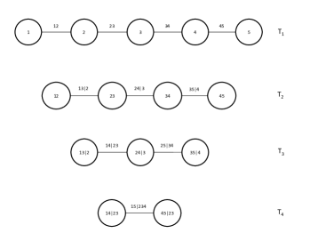
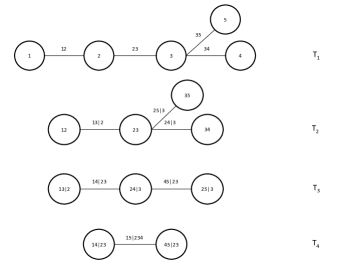
Figure 1: Examples of five-dimensional regular vines: a drawable vine (left) and a non-classified regular vine (right).

The number of terms in the third product is equal to $d-\ell$. For each triple $(i,j,v)$ in the product, $v$ is a subset of $\{1,\ldots,d\}\setminus\{i,j\}$ with exactly $\ell-1$ elements. The precise list of combinatorial rules that the system of triples $(i,j,v)$ must obey makes them constitute a regular vine as in Bedford and Cooke (2001, 2002). Examples of two such structures in dimension five are given in Figure 1.

Assume that for a specific choice of $(i,j,v)$, the copula density $c_{ij|v}$ does not depend on the value of the conditioning argument $x_{v}$, that is, $c_{ij|v}(u_{i},u_{j}|x_{v})$ is constant in $x_{v}$. Since the corresponding copula $C_{ij|v}(\cdot,\cdot|x_{v})$ is equal to the joint distribution function of $(F_{i|v}(X_{i}|X_{v}),F_{j|v}(X_{j}|X_{v}))$ given $X_{v}=x_{v}$, we find that the random pair $(F_{i|v}(X_{i}|X_{v}),F_{j|v}(X_{j}|X_{v}))$ must be independent of the random vector $X_{v}$. Obviously, the converse must hold as well. In that case, equations (3) and (4) simplify to

(6) $$f_{i|j\cup v}(x_{i}|x_{j},x_{v}) =c_{ij|v}\{F_{i|v}(x_{i}|x_{v}),F_{j|v}(x_{j}|x_{v})\}\,f_{i|v}(x_{i}|x_{v}),$$

(7) $$F_{i|j\cup v}(x_{i}|x_{j},x_{v}) =C_{ij|v}^{[2]}\{F_{i|v}(x_{i}|x_{v}),F_{j|v}(x_{j}|x_{v})\}.$$

If it is true for all triples $(i,j,v)$ in the regular vine in (5), we arrive at the pair-copula construction (Joe, 1996; Kurowicka and Cooke, 2006)

(8) $$f(x_{1},\ldots,x_{d})=\prod_{k=1}^{d}f_{k}(x_{k})\,\prod_{\ell=1}^{d-1}\prod_{(i,j,v)}c_{ij|v}\{F_{i|v}(x_{i}|x_{v}),F_{j|v}(x_{j}|x_{v})\},$$

that provides a decomposition of a $d$-variate density in terms of $d$ univariate and $d(d-1)/2$ bivariate copula densities. The pair-copula construction corresponding to the drawable vine in the left panel of Figure 1 is

$$c\{F_{1}(x_{1}),\ldots,F_{5}(x_{5})\}$$

$$= c_{12}\{F_{1}(x_{1}),F_{2}(x_{2})\}\ c_{23}\{F_{2}(x_{2}),F_{3}(x_{3})\}\ c_{34}\{F_{3}(x_{3}),F_{4}(x_{4})\}\ c_{45}\{F_{4}(x_{4}),F_{5}(x_{5})\}$$

$$c_{13|2}\{F_{1|2}(x_{1}|x_{2}),F_{3|2}(x_{3}|x_{2})\}\ c_{24|3}\{F_{2|3}(x_{2}|x_{3}),F_{4|3}(x_{4}|x_{3})\}\ c_{35|4}\{F_{3|4}(x_{3}|x_{4}),F_{5|4}(x_{5}|x_{4})\}$$

$$c_{14|23}\{F_{1|23}(x_{1}|x_{2},x_{3}),F_{4|23}(x_{4}|x_{2},x_{3})\}\ c_{25|34}\{F_{2|34}(x_{2}|x_{3},x_{4}),F_{5|34}(x_{5}|x_{3},x_{4})\}$$

$$c_{15|234}\{F_{1|234}(x_{1}|x_{2},x_{3},x_{4}),F_{5|234}(x_{5}|x_{2},x_{3},x_{4})\}.$$

The assumption that the pair-copulae do not depend on the value of the conditioning argument is a nonparametric shape constraint, that is satisfied for instance by the multivariate Student’s t and Clayton copulae (Hobæk Haff et al., 2010). Even if the assumption does not hold in general, it still provides a reasonable approximation to the true distribution in many cases.

3 Empirical pair-copula

3.1 Estimator

Let $X_{t}=(X_{1t},\ldots,X_{dt})$, for $t=1,\ldots,n$, be a $d$-variate random sample from a distribution function $F$ with density $f$, admitting a pair-copula construction (8) with a known regular vine structure. Choice of the vine structure is a difficult problem, which we will address in Section 4.2. Consider the ground level normalized ranks

$$\hat{U}_{itn}=\frac{1}{n+1}\sum_{s=1}^{n}I(X_{is}\leq X_{it})\qquad(i=1,\ldots,d;\ t=1,\ldots,n).$$

The ground level empirical pair-copula is simply the classical empirical copula

$$\hat{C}_{ij,n}(u_{i},u_{j})=\frac{1}{n}\sum_{t=1}^{n}I\bigl{(}\hat{U}_{itn}\leq u_{i},\,\hat{U}_{jtn}\leq u_{j}\bigr{)}\qquad(i,j\in\{1,\ldots,d\};\ i\neq j).$$

Use finite differencing to obtain an estimator of the conditional distribution function: writing $\hat{C}_{ij,n}(A)=n^{-1}\sum_{t=1}^{n}I\{(\hat{U}_{itn},\hat{U}_{jtn})\in A\}$ for $A\subset\mathbb{R}^{2}$ and given a bandwidth $h>0$, first put

$$\hat{C}_{ij,n}^{[2]}(u_{i},u_{j}) = \frac{\hat{C}_{ij,n}\bigl{(}[0,u_{i}]\times[u_{j}-h,u_{j}+h]\bigr{)}}{\hat{C}_{ij,n}\bigl{(}[0,1]\times[u_{j}-h,u_{j}+h]\bigr{)}}$$

$$= \frac{\sum_{s=1}^{n}I\bigl{(}\hat{U}_{isn}\leq u_{i},\,|\hat{U}_{jsn}-u_{j}|\leq h\bigr{)}}{\sum_{s=1}^{n}I\bigl{(}|\hat{U}_{jsn}-u_{j}|\leq h\bigr{)}},$$

and then, following (2),

$$\hat{F}_{i|j,n}(X_{it}|X_{jt}) = \hat{C}_{ij,n}^{[2]}(\hat{U}_{itn},\hat{U}_{jtn})$$

$$= \frac{\sum_{s=1}^{n}I\bigl{(}\hat{U}_{isn}\leq\hat{U}_{itn},\,|\hat{U}_{jsn}-\hat{U}_{jtn}|\leq h\bigr{)}}{\sum_{s=1}^{n}I\bigl{(}|\hat{U}_{jsn}-\hat{U}_{jtn}|\leq h\bigr{)}}.$$

The denominator of (3.1) is approximately equal to $2nh$, except at the borders, where it is smaller, providing a boundary correction. As the smoothing step in (3.1) takes place on a uniform $(0,1)$ scale, the choice of bandwidth $h$ does not depend on the marginal distributions; in fact, (3.1) is a kind of nearest-neighbour estimator. Bandwidth selection will be addressed in Section 3.4, where it will be seen that a slight degree of undersmoothing is advizable.

For higher levels, we proceed recursively, exploiting the assumption that the pair-copulae do not depend on the value of the conditioning argument. The unwinding of the recursion depends on the given vine structure. Let $(i,j,v)$ be a triple in the vine decomposition (8); in particular, $v$ is a subset of $\{1,\ldots,d\}$ and $i$ and $j$ are distinct elements of $\{1,\ldots,d\}\setminus v$. Suppose that the estimators $\hat{F}_{k|v,n}(X_{kr}|X_{vr})$ have been defined for $k\in\{i,j\}$ and $r=1,\ldots,n$; here $X_{vr}$ denotes the random vector $(X_{mr}:m\in v)$. The normalized ranks of the estimated conditional probabilities are

(11) $$\hat{U}_{k|v,tn}=\frac{1}{n+1}\sum_{r=1}^{n}I\{\hat{F}_{k|v,n}(X_{kr}|X_{vr})\leq\hat{F}_{k|v,n}(X_{kt}|X_{vt})\}\\ (k\in\{i,j\};\ t=1,\ldots,n).$$

The empirical pair-copula is then defined by

(12) $$\hat{C}_{ij|v,n}(u_{i},u_{j})=\frac{1}{n}\sum_{s=1}^{n}I\bigl{(}\hat{U}_{i|v,sn}\leq u_{i},\,\hat{U}_{j|v,sn}\leq u_{j}\bigr{)}.$$

Again, apply finite differencing to get hold on the conditional distributions: first,

$$\hat{C}_{ij|v,n}^{[2]}(u_{i},u_{j}) = \frac{\hat{C}_{ij|v,n}\bigl{(}[0,u_{i}]\times[u_{j}-h,u_{j}+h]\bigr{)}}{\hat{C}_{ij|v,n}\bigl{(}[0,1]\times[u_{j}-h,u_{j}+h]\bigr{)}}$$

$$= \frac{\sum_{s=1}^{n}I\bigl{(}\hat{U}_{i|v,sn}\leq u_{i},\,|\hat{U}_{j|v,sn}-u_{j}|\leq h\bigr{)}}{\sum_{s=1}^{n}I\bigl{(}|\hat{U}_{j|v,sn}-u_{j}|\leq h\bigr{)}}$$

and then, following (7),

(14) $$\hat{F}_{i|v\cup j,n}(X_{it}|X_{v\cup j,t}) = \hat{C}_{ij,n}^{[2]}(\hat{U}_{i|v,tn},\hat{U}_{j|v,tn})$$

$$= \frac{\sum_{s=1}^{n}I\bigl{(}\hat{U}_{i|v,sn}\leq\hat{U}_{i|v,tn},\,|\hat{U}_{j|v,sn}-\hat{U}_{j|v,tn}|\leq h\bigr{)}}{\sum_{s=1}^{n}I\bigl{(}|\hat{U}_{j|v,sn}-\hat{U}_{j|v,tn}|\leq h\bigr{)}}.$$

We proceed this way, recursively from the ground level, $\ell=1$, where $v$ is the empty set, to the top level, $\ell=d-1$, with $v$ consisting of $d-2$ elements, adding a variable for each level.

The empirical pair-copula estimates the pair-copula distribution functions. Kolbjørnsen and Stien (2008) propose a nonparametric estimator for the pair-copula density, with variables transformed to the Gaussian rather than the uniform domain, to mitigate boundary effects.

3.2 Asymptotic distribution

Let $(i,j,v)$ be a triple in the vine decomposition (8). Because of the assumption that the copula of the conditional distribution of $(X_{i},X_{j})$ given $X_{v}=x_{v}$ does not depend on the value of $x_{v}$, the pair-copula $C_{ij|v}$ is in fact equal to the unconditional distribution function of the random pair $(F_{i|v}(X_{i}|X_{v}),F_{j|v}(X_{j}|X_{v}))$:

$$\operatorname{pr}\{F_{i|v}(X_{i}|X_{v})\leq u_{i},\,F_{j|v}(X_{j}|X_{v})\leq u_{j}\}$$

$$= \int\operatorname{pr}\{F_{i|v}(X_{i}|X_{v})\leq u_{i},\,F_{j|v}(X_{j}|X_{v})\leq u_{j}\mid X_{v}=x_{v}\}\,f_{v}(x_{v})\,\mathrm{d}x_{v}$$

$$= \int C_{ij|v}(u_{i},u_{j}|x_{v})\,f_{v}(x_{v})\,\mathrm{d}x_{v}$$

$$= \int C_{ij|v}(u_{i},u_{j})\,f_{v}(x_{v})\,\mathrm{d}x_{v}=C_{ij|v}(u_{i},u_{j}).$$

Therefore, it is reasonable to expect that it can be estimated at the parametric rate $O_{p}(n^{-1/2})$.

Define the random variables

(15) $$U_{k|v,t}=F_{k|v}(X_{kt}|X_{vt})\qquad(k\in\{i,j\};\ t=1,\ldots,n).$$

We conjecture that under suitable smoothness conditions on the copula density $c$ and growth conditions on the bandwidth sequence $h=h_{n}$, the empirical pair-copula (12) satisfies

(16) $$\mathbb{C}_{ij|v,n}(u_{i},u_{j}) = n^{1/2}\{\hat{C}_{ij|v,n}(u_{i},u_{j})-C_{ij|v}(u_{i},u_{j})\}$$

$$= n^{-1/2}\sum_{t=1}^{n}\{I(U_{i|v,t}\leq u_{i},U_{j|v,t}\leq u_{j})-C_{ij|v}(u_{i},u_{j})\}$$

$$\quad\mbox{}-C_{ij|v}^{[1]}(u_{i},u_{j})\,n^{-1/2}\sum_{t=1}^{n}\{I(U_{i|v,t}\leq u_{i})-u_{i}\}$$

$$\quad\mbox{}-C_{ij|v}^{[2]}(u_{i},u_{j})\,n^{-1/2}\sum_{t=1}^{n}\{I(U_{j|v,t}\leq u_{j})-u_{j}\}+o_{p}(1).$$

The expansion (16) is suggested by tedious calculations and supported by extensive simulations summarized in Section 3.4.

Incidentally, the right-hand side of (16) coincides with the expansion for the empirical copula process of the unobservable random pairs $(U_{i|v,t},U_{j|v,t})$, for $t=1,\ldots,n$. This empirical copula would arise if the estimated conditional distribution functions $\hat{F}_{k|v,n}$ in equation (11) were replaced by the true ones, $F_{k|v}$, with normalized ranks

(17) $$U_{k|v,tn}=\frac{1}{n+1}\sum_{r=1}^{n}I\{F_{k|v,n}(X_{kr}|X_{vr})\leq F_{k|v,n}(X_{kt}|X_{vt})\}\\ (k\in\{i,j\};\ t=1,\ldots,n),$$

and the empirical copula

(18) $$C_{ij|v,n}(u_{i},u_{j})=\frac{1}{n}\sum_{t=1}^{n}I\bigl{(}U_{i|v,tn}\leq u_{i},\,U_{j|v,tn}\leq u_{j}\bigr{)},$$

without hats. By theory going back to Rüschendorf (1976) and Stute (1984), equation (16) holds when the empirical pair-copula $\hat{C}_{ij|v,n}$ (12) is replaced by the empirical copula $C_{ij|v,n}$ (18). As we are working with the ranks of the variables $\hat{F}_{k|v,n}(X_{kt}|X_{vt})$ ($t=1,\ldots,n$), rather than the values themselves, it is intuitively not unreasonable to expect that replacing $\hat{F}_{k|v,n}$ by $F_{k|v,n}$ makes no difference asymptotically. For some recent references on the empirical copula see Fermanian et al. (2004), Tsukahara (2005), van der Vaart and Wellner (2007), and Segers (2012).

The expansion in (16) implies that the empirical pair-copula is asymptotically normal,

(19) $$n^{1/2}\{\hat{C}_{ij|v,n}(u_{i},u_{j})-C_{ij|v}(u_{i},u_{j})\}\stackrel{{\scriptstyle d}}{{\rightarrow}}N\bigl{(}0,\sigma_{ij|v}^{2}(u_{i},u_{j})\bigr{)}\qquad(n\to\infty),$$

with asymptotic variance equal to

(20) $$\sigma_{ij|v}^{2}(u_{i},u_{j})=C_{ij|v}(1-C_{ij|v})+(C_{ij|v}^{[1]})^{2}\,u_{i}(1-u_{i})+(C_{ij|v}^{[2]})^{2}\,u_{j}(1-u_{j})\\ -C_{ij|v}^{[1]}\,C_{ij|v}(1-u_{i})-C_{ij|v}^{[2]}\,C_{ij|v}(1-u_{j})+C_{ij|v}^{[1]}\,C_{ij|v}^{[2]}\,(C_{ij|v}-u_{i}u_{j}),$$

where the arguments $(u_{i},u_{j})$ of $C_{ij|v}$ and its partial derivatives have been suppressed in the notation. Replacing $C_{ij|v}$ and its derivatives by the estimators (12)–(3.1) yields a plug-in estimator $\hat{\sigma}_{ij|v}^{2}(u_{i},u_{j})$ for the asymptotic variance.

3.3 Resampling

The empirical pair-copula will most naturally be used for interval estimation and hypothesis tests. To be able to derive critical values, one needs resampling procedures. Here we propose the multiplier bootstrap for the empirical pair-copula process in (16). It resembles the approach for the ordinary empirical copula process, proposed by Rémillard and Scaillet (2009) and studied in Bücher and Dette (2010) and Segers (2012).

Consider first the bivariate empirical process

$$\alpha_{ij|v,n}(u_{i},u_{j})=n^{-1/2}\sum_{t=1}^{n}\bigl{\{}I(U_{i|v,t}\leq u_{i},\,U_{j|v,t}\leq u_{j})-C_{ij|v}(u_{i},u_{j})\bigr{\}},$$

based upon the random variables $U_{k|v,t}$ from (15). Let $\xi_{1},\ldots,\xi_{n}$ be independent and identically distributed random variables, independent of the original sample $X_{1},\ldots,X_{n}$, with mean zero, unit variance, and a finite absolute moment of some order larger than two, for instance from the standard normal distribution. By Lemma A.1 in Rémillard and Scaillet (2009), the process

$$\alpha_{ij|v,n}^{\prime}(u_{i},u_{j}) = n^{-1/2}\sum_{t=1}^{n}\xi_{t}\,\bigl{\{}I(U_{i|v,tn}\leq u_{i},\,U_{j|v,tn}\leq u_{j})-C_{ij|v,n}(u_{i},u_{j})\bigr{\}}$$

$$= n^{-1/2}\sum_{t=1}^{n}\bigl{(}\xi_{t}-\bar{\xi}_{n}\bigr{)}\,I(U_{i|v,tn}\leq u_{i},\,U_{j|v,tn}\leq u_{j})$$

is an asymptotically independent distributional copy of $\alpha_{ij|v,n}$. We therefore propose

$$\hat{\alpha}_{ij|v,n}^{\prime}(u_{i},u_{j})=n^{-1/2}\sum_{t=1}^{n}\bigl{(}\xi_{t}-\bar{\xi}_{n}\bigr{)}\,I\bigl{(}\hat{U}_{i|v,tn}\leq u_{i},\,\hat{U}_{j|v,tn}\leq u_{j}\bigr{)}$$

as a bootstrap resample of $\alpha_{ij|v,n}(u_{i},u_{j})$. In view of equation (16), we then suggest resampling $\mathbb{C}_{ij|v,n}(u_{i},u_{j})$ by

(21) $$\hat{\alpha}_{ij|v,n}^{\prime}(u_{i},u_{j})\\ -\hat{C}_{ij|v,n}^{[1]}(u_{i},u_{j})\,\hat{\alpha}_{ij|v,n}^{\prime}(u_{i},1)-\hat{C}_{ij|v,n}^{[2]}(u_{i},u_{j})\,\hat{\alpha}_{ij|v,n}^{\prime}(1,u_{j}).$$

Repeating the procedure for $B$ independent rows $\xi_{b1},\ldots,\xi_{bn}$, with $b\in\{1,\ldots,B\}$, gives $B$ approximately independent distributional copies of $\alpha_{ij|v,n}(u_{i},u_{j})$, and thus of $\mathbb{C}_{ij|v,n}(u_{i},u_{j})$. The pointwise sample variance of these $B$ resamples may serve as an alternative estimator $\tilde{\sigma}_{ij|v}^{2}(u_{i},u_{j})$ of (20). Two-sided asymptotic confidence intervals for $C_{ij|v}(u_{i},u_{j})$ with confidence level $1-\alpha$ can be obtained by

(22) $$\bigl{[}\hat{C}_{ij|v,n}-n^{-1/2}\hat{q}_{n,1-\alpha/2},\,\hat{C}_{ij|v,n}-n^{-1/2}\hat{q}_{n,\alpha/2}\bigr{]},$$

where $\hat{q}_{n,\beta}$ is either the bootstrap estimate of the $\beta$-quantile of $\mathbb{C}_{ij|v,n}(u_{i},u_{j})$, that is, the $\beta$-percentile of the bootstrap samples, or $\tilde{\sigma}_{ij|v}\,\Phi^{-1}(\beta)$, where $\Phi^{-1}$ is the quantile function of the standard normal distribution.

3.4 Simulation studies of the asymptotic distribution

We have substantiated the conjectured expansion (16), limiting distribution (19), with (20), and the resampling procedure from Section 3.3 through simulation. The study includes different types of structures, pair-copula models and parameter values. In each experiment, we have generated $1,000$ samples of size $n$ from the model in question, with $n$ ranging from $100$ to $100,000$. For each sample, we have computed $\mathbb{C}_{ij|v,n}(u_{i},u_{j})$, as well as the absolute difference between $\mathbb{C}_{ij|v,n}(u_{i},u_{j})$ and the expansion (16), in a set of chosen points $(u_{i},u_{j})$, at given levels of the structure. The models of the study are five-dimensional and comprise the drawable and regular vines of Figure 1, and a canonical vine, which is another special case. The latter two are Gaussian, and the former either Gaussian, Student’s t or Gumbel. The parameters of all the Gumbel copulae are $\theta=1$$\cdot$$5$. Further, the Gaussian and Student’s t correlations are $\rho$, $\rho/(1+\rho)$, $\rho/(1+2\rho)$ and $\rho/(1+3\rho)$ at the first, second, third and fourth level, respectively, with $\rho=0$$\cdot$$2$, $0$$\cdot$$5$, $0$$\cdot$$8$. The corresponding degrees of freedom of the latter are $\nu$, $\nu+1$, $\nu+2$ and $\nu+3$, with $\nu=6$.

According to (16), the absolute difference between the left and right hand sides should decrease and eventually vanish as $n$ increases. The top row of Figure 2 shows the mean of these differences in the point $(0$$\cdot$$3,0$$\cdot$$7)$, over the simulations from the Gaussian drawable vine with $\rho=0$$\cdot$$5$, for growing $n$, on log-log scale. Indeed, these decrease, though rather slowly. The rate of convergence appears to be approximately of the same order as for the ordinary empirical copula process, namely $n^{-1/4}$, which is to be expected.

Furthermore, we have tested the limiting distribution (19) of $\mathbb{C}_{ij|v,n}(u_{i},u_{j})$ with variance (20), using the Kolmogorov-Smirnov goodness-of-fit test. Table 1 shows the corresponding p-values in the three points $(0$$\cdot$$1,0$$\cdot$$3)$, $(0$$\cdot$$4,0$$\cdot$$2)$ and $(0$$\cdot$$7,0$$\cdot$$8)$ for a selection of models and levels, with $\rho=0$$\cdot$$5$ and $n=1,000$. The consistently high p-values indicate that the assumed distribution fits the samples well. This is confirmed by normal QQ-plots and histograms of the samples, superposed by the asymptotic probability density functions. These are displayed in the lower two rows of Figure 2 for the Gaussian drawable vine with $n=1,000$. Examples with other structures and copulae may be found in the supplement.

Structure	Copula	Level	p-value
			(0$\cdot$1,0$\cdot$3)	(0$\cdot$4,0$\cdot$2)	(0$\cdot$7,0$\cdot$8)
Drawable	Gaussian	2	0$\cdot$54	0$\cdot$48	0$\cdot$67
		3	0$\cdot$40	0$\cdot$70	0$\cdot$69
		4	0$\cdot$26	0$\cdot$44	0$\cdot$36
	Student’s t	2	0$\cdot$47	0$\cdot$65	0$\cdot$51
	Gumbel	2	0$\cdot$37	0$\cdot$91	0$\cdot$45
Canonical	Gaussian	3	0$\cdot$37	0$\cdot$45	0$\cdot$44
Regular	Gaussian	4	0$\cdot$35	0$\cdot$61	0$\cdot$41

Table 1: P-values from the Kolmogorov-Smirnov goodness-of-fit tests on the simulated processes $\mathbb{C}_{ij|v,n}(u_{i},u_{j})$ with $n=1,000$, in the points (0$\cdot$1,0$\cdot$3), (0$\cdot$4,0$\cdot$2) and (0$\cdot$7,0$\cdot$8), for different vine structures, copula models and levels

As seen from (3.1) and (14), the estimators depend on a bandwidth parameter $h_{n}$. This bandwidth should obviously be proportional to some power of $n^{-1}$, at least $n^{-1/2}$ to guarantee consistent estimators. Viewing $\hat{C}_{ij,n}^{[2]}(u_{i},u_{j})$ and $\hat{C}_{ij|v,n}^{[2]}(u_{i},u_{j})$ as predictions of the conditional expectations $\operatorname{E}(I(U_{i}\leq u_{i})|U_{j}=u_{j}))$ and $\operatorname{E}(I(U_{i|v}\leq u_{i})|U_{j|v}=u_{j}))$, respectively, one could construct a cross-validation procedure for bandwidth selection. However, this is non-trivial since the observations are indicator functions, the choice of points $(u_{i},u_{j})$ is not obvious and there are up to $(d-1)(d-2)$ predictors to evaluate.

In order to investigate the influence of the bandwidth on the estimators, we have repeated the simulation of the Gaussian drawable vine with each of the three bandwidths $h_{n}=n^{-\frac{1}{5}}$, $n^{-\frac{1}{4}}$ and $0$$\cdot$$5n^{-\frac{1}{3}}$. The first of these is proportional to Silverman’s rule. The other two are undersmoothing alternatives. As mentioned earlier, the optimal choice of bandwidth does not depend on the margins, but only on the dependence structure. For $\rho=0$$\cdot$$2$, the estimators behave well for all three bandwidths, but for higher dependencies, i.e. $\rho=0$$\cdot$$5$ and $0$$\cdot$$8$, $h_{n}=0$$\cdot$$5n^{-\frac{1}{3}}$ is without a doubt the only sensible choice. We have therefore used that bandwidth throughout the paper. Intuitively, it makes sense to undersmooth the estimators, i.e. to minimize the bias at the expense of the variance. The pointwise estimates of the conditional distributions may then differ considerably from the true values, but the copula estimator will average out these discrepancies.

It remains to test the proposed resampling procedure. We have simulated from the Gaussian, Student’s t and Gumbel drawable vines from before, in dimension $d=4$, with $\rho=0$$\cdot$$5$ and $n=1,000$. For each sample, we have generated $B=1,000$ multiplier bootstrap estimates of the confidence interval (22) of the top level copula $C_{14|23}$, evaluated in $(0$$\cdot$$4,0$$\cdot$$2)$, with $\alpha=\{0$$\cdot$$1,0$$\cdot$$05,0$$\cdot$$01\}$, using both approaches, as well as plug-in estimates, based on $\hat{\sigma}_{ij|v}^{2}$.

As suggested earlier, parametric estimators are more efficient when the model is correctly specified, or at least close to the truth. However, we believe that the empirical estimator is more robust. Therefore, we have computed corresponding percentile confidence intervals based on parametric bootstrap, assuming both correct and incorrect copula families in the lower two levels, but always the true family for the copula of interest. More specifically, we estimated the intervals for the Gaussian model, assuming first the true model, and then Gumbel copulae in the first two levels. We repeated this for the Student’s t model with Gumbel copulae, and for the Gumbel model with Gaussian copulae. The estimator we have used is the stepwise semiparametric estimator; see for instance Hobæk Haff (2012).

Table 2 shows the confidence intervals’ average length and actual coverage, i.e. the fraction of intervals that contain the true value of $C_{12|34}(0$$\cdot$$4,0$$\cdot$$2)$. The ones based on the multiplier bootstrap percentiles are shorter than the symmetric ones. Further, the plug-in estimator $\hat{\sigma}_{14|23}^{2}$ is surprisingly good. Of course, all these intervals are longer than the ones obtained with the parametric estimator. Moreover, their actual coverage is consistently higher than the nominal one. However, the misspecified models produce intervals with substantially lower coverage than the chosen confidence levels. Hence, tests based on the empirical estimator are expected to be conservative, and thus less powerful than parametric equivalents, but on the other hand more robust towards misspecifications in lower levels. Another advantage of the multiplier bootstrap scheme is that it is much faster than the parametric one, especially for the Student’s t model. Also note that for this particular model, the parametric intervals made under the true model assumptions have smaller coverage than the nominal one, which probably means that $B=1,000$ is insufficient in this case. Naturally, the misspecifications in the above experiments are not very realistic, but merely meant as an illustration of how errors propagate from level to level. In practice, one should be able to choose reasonably well at least at the first level.

We repeated the above simulations for the Gaussian model with $B=500$ and with $n=10,000$. The results were as expected. When $n$ increases, the interval lengths obviously decrease, whereas the actual coverage becomes more varying for smaller $B$. We therefore use $n=B=1,000$ in the remaining sections.

Model	$\alpha$	Non-parametric			Parametric
		Percentile	Symmetric	Plug-in	Correct	Incorrect
Gaussian	0$\cdot$1	0$\cdot$940(2$\cdot$1)	0$\cdot$940(2$\cdot$1)	0$\cdot$940(2$\cdot$1)	0$\cdot$900(1$\cdot$1)	0$\cdot$860(1$\cdot$1)
	0$\cdot$05	0$\cdot$970(2$\cdot$5)	0$\cdot$980(2$\cdot$5)	0$\cdot$980(2$\cdot$5)	0$\cdot$950(1$\cdot$3)	0$\cdot$920(1$\cdot$3)
	0$\cdot$01	0$\cdot$990(3$\cdot$2)	0$\cdot$990(3$\cdot$2)	0$\cdot$990(3$\cdot$3)	0$\cdot$990(1$\cdot$7)	0$\cdot$970(1$\cdot$7)
Student’s t	0$\cdot$1	0$\cdot$910(2$\cdot$1)	0$\cdot$910(2$\cdot$1)	0$\cdot$910(2$\cdot$1)	0$\cdot$890(1$\cdot$2)	0$\cdot$000(1$\cdot$1)
	0$\cdot$05	0$\cdot$950(2$\cdot$5)	0$\cdot$950(2$\cdot$5)	0$\cdot$950(2$\cdot$5)	0$\cdot$940(1$\cdot$4)	0$\cdot$000(1$\cdot$4)
	0$\cdot$01	0$\cdot$990(3$\cdot$2)	0$\cdot$990(3$\cdot$3)	0$\cdot$990(3$\cdot$3)	0$\cdot$980(1$\cdot$9)	0$\cdot$000(1$\cdot$8)
Gumbel	0$\cdot$1	0$\cdot$910(2$\cdot$0)	0$\cdot$910(2$\cdot$0)	0$\cdot$910(2$\cdot$0)	0$\cdot$910(1$\cdot$0)	0$\cdot$680(1$\cdot$0)
	0$\cdot$05	0$\cdot$960(2$\cdot$4)	0$\cdot$960(2$\cdot$4)	0$\cdot$960(2$\cdot$4)	0$\cdot$960(1$\cdot$2)	0$\cdot$790(1$\cdot$2)
	0$\cdot$01	0$\cdot$990(3$\cdot$1)	0$\cdot$990(3$\cdot$1)	0$\cdot$990(3$\cdot$1)	0$\cdot$990(1$\cdot$6)	0$\cdot$910(1$\cdot$5)

Table 2: Coverage of the estimated confidence intervals for $C_{14|23}(0$$\cdot$$4,0$$\cdot$$2)$ in the Gaussian, Student’s t and Gumbel models with $n=1,000$. The average lengths, in parentheses, are multiplied by $10^{2}$.

4 Methods derived from the empirical pair-copula

4.1 Estimating the conditional Spearman correlation

The Spearman correlation $\rho_{S}$ of the bivariate copula $C$ of a random pair $(U,V)$ with uniform $(0,1)$ margins can be expressed as

$$\rho_{S}(C)=12\int_{[0,1]^{2}}C(u,v)\,\mathrm{d}(u,v)-3=\operatorname{cor}(U,V).$$

Similarly, $\rho_{S}(C_{ij|v})$ is a measure of association between $X_{i}$ and $X_{j}$, conditionally on $X_{v}$. This quantity can be estimated by the plug-in estimator $\rho_{S}(\hat{C}_{ij|v,n})=12\int\hat{C}_{ij|v,n}-3$, which is approximately equal to the sample correlation of the pairs $(\hat{U}_{i|v,tn},\hat{U}_{j|v,tn})$, for $t=1,\ldots,n$. The expansion of the empirical pair-copula process in (16) implies that

(23) $$n^{1/2}\{\rho_{S}(\hat{C}_{ij|v,n})-\rho_{S}(C_{ij|v})\}\stackrel{{\scriptstyle d}}{{\rightarrow}}12\int_{[0,1]^{2}}\mathbb{C}_{ij|v}(u_{i},u_{j})\,\mathrm{d}(u_{i},u_{j}),$$

where $\mathbb{C}_{ij|v}$, the conjectured large-sample limit of $\mathbb{C}_{ij|v,n}$, is a centred Gaussian process on $[0,1]^{2}$ with covariance function determined by the right-hand side of (16). The limiting random variable in (23) is a centred normal random variable with variance

$$\sigma_{\rho}^{2}=144\int_{[0,1]^{2}}\int_{[0,1]^{2}}\operatorname{cov}\{\mathbb{C}_{ij|v}(u_{i},u_{j}),\,\mathbb{C}_{ij|v}(u_{i}^{\prime},u_{j}^{\prime})\}\,\mathrm{d}(u_{i},u_{j})\,\mathrm{d}(u_{i}^{\prime},u_{j}^{\prime}).$$

This variance can be estimated either by a plug-in estimator or via the multiplier resampling scheme described in Section 3.3. The latter procedure consists in resampling $\mathbb{C}_{ij|v,n}$ and integrating it either by numerical or Monte Carlo integration over $[0,1]^{2}$. One may then estimate $\sigma_{\rho}^{2}$ by the sample variance of the $B$ resamples of $12\int\mathbb{C}_{ij|v}$. Further, confidence intervals for $\rho_{S}(C_{ij|v,n})$ can be constructed either via the normal approximation with estimated variance $\sigma_{\rho}^{2}$ or by using resample percentiles.

In order to verify (23), we have simulated from the same four-dimensional models as in the last part of Section 3.4, computing (23) for each of the $1,000$ samples. The p-values from the Kolmogorov-Smirnov tests are $0$$\cdot$$89$, $0$$\cdot$$92$ and $0$$\cdot$$68$, respectively, for the three models, which clearly agrees with the conjecture. Normal QQ-plots and histograms are shown in the supplement.

Moreover, we have tested the suggested resampling scheme for $12\int\mathbb{C}_{14|23}$ in the same way as in Section 3.4. The corresponding results, shown in the supplement, are very similar. The confidence intervals based on the empirical estimator are longer and have larger actual coverage than the parametric equivalents, whereas the latter are non-robust towards misspecifications in lower levels. Once more, the intervals based on the multiplier bootstrap percentiles appear to be the best of the empirical ones. The plug-in estimator of the variance $\sigma_{\rho}^{2}$ is also rather good, but computationally much slower than the multiplier bootstrap.

4.2 Vine structure selection

Selecting the structure of a pair-copula construction consists in choosing which variables to associate with a pair-copula at each level. As the model uncertainty increases with the level, the state of the art is to try to capture as much of the dependence as possible in the lower levels of the structure. Aas et al. (2009) propose ordering the variables of a drawable vine in the way that maximizes the tail dependencies at the ground level, while Dissmann et al. (2011) suggest a model selection algorithm for more general regular vines, that maximizes the sum of absolute values of Kendall’s $\tau$ coefficients at each level. Both these schemes require the simultaneous choice and estimation of parametric copulae. At the ground level, the latter algorithm only uses the sample Kendall’s $\tau$s, and therefore does not call for assumptions about the pair-copulae. However, from the second level on, the $\tau$s involve the unobserved variables $F_{i|v}(X_{i}|X_{v})$, that are estimated parametrically from the copulae in the previous level via (7). Inadequate choices of copulae may thus influence the structure selection at the higher levels.

We propose a more robust model selection scheme, based on our nonparametric estimate of the Spearman correlation $\rho_{S}$.

1. Compute the ground level normalized ranks $\hat{U}_{itn}$ ($t=1,\ldots,n)$.

2. Compute $\rho_{S}(\hat{C}_{ij,n})$ for all pairs $\{i,j\}\subset\{1,\ldots,d\}$ such that $i<j$.

3. Select the spanning tree $T_{1}$ on $\{1,\ldots,d\}$ that maximizes $\sum_{\{i,j\}\in T_{1}}|\rho_{S}(\hat{C}_{ij,n})|$.

4. Estimate $\hat{U}_{i|j,tn}$ and $\hat{U}_{j|i,tn}$ for all selected pairs $\{i,j\}$, using (3.1).

5. For levels $\ell=2,\ldots,d-1$:

   1. Compute $\rho_{S}(\hat{C}_{ij|v,n})$ for all possible pairs $\{i,j\}$.

   2. Select the spanning tree $T_{\ell}$ that maximizes $\sum_{\{i,j\}\in T_{\ell}}|\rho_{S}(\hat{C}_{ij|v,n})|$.

   3. Estimate $\hat{U}_{i|j\cup v,tn}$ and $\hat{U}_{j|i\cup v,tn}$ for all selected pairs $\{i,j\}$, using (14).

The above algorithm is strongly inspired by Dissmann et al. (2011), who also explain the concept of possible pairs. We merely estimate the copulae and conditional distributions nonparametrically rather than parametrically and use Spearman’s $\rho_{S}$ instead of Kendall’s $\tau$. The substitution of dependence measures should not influence the results too much. When the model is well specified, one would therefore expect the two algorithms to select virtually the same structure.

The algorithm is put into practice in Section 5.1, where it is found to impose quite a reasonable structure on a set of financial variables.

4.3 Testing for conditional independence

The number of parameters in a pair-copula construction grows rapidly with increasing dimension $d$. Identifying independence copulae in the structure is one way of reducing this number. One may therefore add tests for conditional independence as a step in the model selection algorithm of Section 4.2.

In case $C_{ij|v}$ is the independence copula, equation (16) implies that the asymptotic distribution of $\hat{C}_{ij|v,n}$ is the same as the one of the bivariate empirical copula under independence. In other words, the random vectors $(\hat{U}_{i|v,tn},\hat{U}_{j|v,tn})$ for $t\in\{1,\ldots,n\}$ behave in distribution as the sample of bivariate normalized ranks from a random sample of a bivariate distribution with independent components. Therefore, rank-based tests for independence can be applied without adjustment of the critical values.

We propose to test the null hypothesis of conditional independence of $X_{i}$ and $X_{j}$, given $X_{v}$, by the Cramér-von Mises test statistic

$$\int_{[0,1]^{2}}\mathbb{C}_{ij|v,n}^{2}(u_{i},u_{j})\,\mathrm{d}\hat{C}_{ij|v,n}(u_{i},u_{j})=\frac{1}{n}\sum_{t=1}^{n}\mathbb{C}_{ij|v,n}^{2}(\hat{U}_{i|v,tn},\hat{U}_{j|v,tn}),$$

where $\mathbb{C}_{ij|v,n}(u_{i},u_{j})=n^{1/2}\{\hat{C}_{ij|v,n}(u_{i},u_{j})-u_{i}u_{j}\}$ is the empirical pair-copula process under the null hypothesis of conditional independence, that is, $C_{ij|v}(u_{i},u_{j})=u_{i}u_{j}$ for all $(u_{i},u_{j})\in[0,1]^{2}$. Under the null hypothesis, the limit distribution of the test statistic is distribution free and is given by $\int_{[0,1]^{2}}\mathbb{C}^{2}(u,v)\,\mathrm{d}(u,v)$, where $\mathbb{C}$ is the limiting empirical copula process under independence. Critical values of the test statistic can be obtained by Monte Carlo estimation based on random samples from a distribution with independent components.

Once more, we have compared our test with parametric equivalents, based on parametric bootstrap, on the four-dimensional models from Section 3.4, but with the top level copula $C_{14|23}(u_{1},u_{4})=u_{1}u_{4}$. Table 3 shows the rejection rates at levels $\alpha=\{0$$\cdot$$1,0$$\cdot$$05,0$$\cdot$$01\}$. Again, the tests based on the empirical estimator appear to be conservative, that is, the rejection rates are consistently lower than the specified levels. As anticipated, the parametric tests are more powerful under correct model assumptions, but the rejection rates are slightly too high for the Student’s t model, which seems to require a higher $B$. Moreover, the rejection rates are too high under incorrect model assumptions, which demonstrates these tests’ lack of robustness.

4.4 Goodness-of-fit testing

In the parametric case, model selection consists in choosing not only the structure, as described in Section 4.1, but also the families of the $d(d-1)/2$ copulae. Goodness-of-fit tests can help to assess whether the selected model represents the dependence structure well. At the ground level, one may simply apply the standard tests, for instance the ones studied in Genest et al. (2009). From the second level on, it becomes more complicated, since the copula arguments are themselves unknown conditional distributions, derived from a cascade of pair-copulae at lower levels.

Following the reasoning of Section 4.3, we propose a Cramér-von Mises goodness-of-fit test, more specifically, the test proposed by Genest and Rémillard (2008), replacing the normalized ranks by our non-parametric estimators of the conditional distributions. Critical values may then be obtained by the bootstrap procedure they describe, again substituting the normalized ranks by our estimators.

Testing this procedure on the top level copula of the four-dimensional Gumbel model from Section 3.4 with $n=1,000$, we obtained rejection rates of $0$$\cdot$$098$, $0$$\cdot$$042$ and $0$$\cdot$$0044$ for the null hypothesis that it is a Gumbel copula at levels $0$$\cdot$$1$, $0$$\cdot$$05$ and $0$$\cdot$$01$, respectively. For the hypotheses that it is Student’s t and Gaussian, the corresponding rates were $0$$\cdot$$90$, $0$$\cdot$$83$, $0$$\cdot$$60$ and $0$$\cdot$$91$, $0$$\cdot$$84$, $0$$\cdot$$62$. Hence the former are clearly rejected, while the true model, Gumbel, is not, as it should be.

Model		Non-parametric	Parametric
	$\alpha$		Correct	Incorrect
Gaussian	0$\cdot$1	0$\cdot$099	0$\cdot$10	0$\cdot$22
	0$\cdot$05	0$\cdot$049	0$\cdot$050	0$\cdot$14
	0$\cdot$01	0$\cdot$0096	0$\cdot$010	0$\cdot$034
Student’s t	0$\cdot$1	0$\cdot$097	0$\cdot$11	0$\cdot$16
	0$\cdot$05	0$\cdot$047	0$\cdot$068	0$\cdot$082
	0$\cdot$01	0$\cdot$0093	0$\cdot$022	0$\cdot$042
Gumbel	0$\cdot$1	0$\cdot$094	0$\cdot$099	0$\cdot$23
	0$\cdot$05	0$\cdot$044	0$\cdot$048	0$\cdot$14
	0$\cdot$01	0$\cdot$0088	0$\cdot$0090	0$\cdot$048

Table 3: Rejection rates from the Cramér-von Mises tests for conditional independence at the third level of the Gaussian, Student’s t and Gumbel models with $n=1,000$

5 Data examples

5.1 Financial data set

The financial data set consists of nine Norwegian and international daily price series from March 25th, 2003, to March 26th, 2006, which corresponds to 1107 observations. These include the Norwegian 5- and 6-year Swap Rates (NI5 and NI6), the 5-year German Government Rate (GI5), the BRIX Norwegian Bond Index (NB) and ST2X Government Bond Index (MM), the WGBI Citigroup World Government Bond Index (IB), the OSEBX Oslo Stock Exchange Main Index (NS), the MSCI Morgan Stanley World Index (IS) and the Standard & Poor Hedge Fund Index (HF). This is a subset of the 19 variables, analyzed in Brechmann et al. (2012), which represent the market portfolio of one of the largest Norwegian financial institutions. We have followed their example, and filtrated each of the series with an appropriate time series model to remove the temporal dependence. Subsequently, we have modelled the standardized residuals with a regular vine.

We selected the vine structure, first with the method proposed in Section 4.2 and then with the method of Dissmann et al. (2011). The two selected structures were actually identical, which is reassuring. The dependence in the ground level appears to be very strong, with Spearman rank correlations that are large in absolute value. In the remaining levels, the Spearman correlations are considerably smaller, and only 9 out of 28 copulae were significantly different from the independence copula at level 0$\cdot$05, according to the test from Section 4.3. Hence, most of the dependence has been captured in the ground level, shown in Figure 3, which was the aim.

The collection of pairs selected by the algorithm at this level is quite reasonable. The three stock indices and the three interest rates are grouped together, whereas the Norwegian bond indices are dependent on the international bond index via the interest rates.

5.2 Precipitation data set

The precipitation set is composed of daily recordings from January 1st, 1990, to December 31st, 2006, at five different meteorological stations in Norway: Vestby, Ski, Lørenskog, Nannestad and Hurdal. This data set was used in both Berg and Aas (2009) and Hobæk Haff (2012). As in those papers, we have modelled only the positive precipitation, discarding all observations for which at least one of the stations has recorded zero precipitation. The remaining 2013 observations appear to be fairly independent in time. We model these with a drawable vine, ordering the stations according to geography. The model is quite natural since the stations are located almost on a straight line, from Vestby in the South to Hurdal in the North; see the map in the supplement. The parametric model used for comparison is the one from Hobæk Haff (2012), with Gumbel copulae at the ground level and subsequently Gaussian ones.

Since rain showers tend to be rather local, one would expect the dependence to be strongest between the closest stations, and decrease with the level, possibly even down to conditional independence. Therefore we have tested the second, third and fourth level copulae for conditional independence, both with the non-parametric test from Section 4.3 and equivalent parametric tests. The Spearman rank correlations at the ground level range from 0$\cdot$82 to 0$\cdot$94, indicating a strong positive dependence. At the second level, they are considerably lower, but the hypothesis of conditional independence is rejected for all copulae, by both tests, which actually agree in the last two levels as well. The conditional copula of the measurements from Vestby and Nannestad, given the two stations in between, is also significantly different from independence. This is not true for Ski and Hurdal, conditioning on Lørenskog and Nannestad, and neither for the top level copula, linking Vestby and Hurdal, conditionally on the three stations in between.

Figure 2: Results for the Gaussian drawable vine with $\rho=0$$\cdot$$5$ at levels 2, 3 and 4 (in columns 1, 2 and 3, respectively). The first row shows the means of the samples of the absolute difference between $\mathbb{C}_{ij|v,n}(0$$\cdot$$3,0$$\cdot$$7)$ and expansion (16), for $n$ from $10^{2}$ to $10^{5}$, on log-log scale (the original values are on the axes). The last two rows display normal QQ-plots and histograms of the samples of $\mathbb{C}_{ij|v,n}(0$$\cdot$$4,0$$\cdot$$2)$ with $n=1,000$, respectively, the latter superposed by the limiting probability density functions from (19).

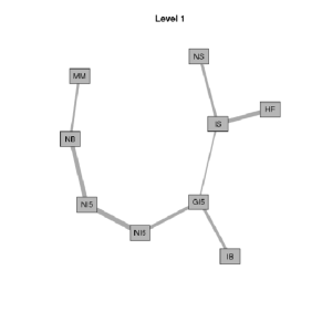
Figure 3: Ground level of the regular vine selected for the financial data in Section 5.1. The thickness of the edges is determined by the absolute value of the corresponding Spearman rank correlations.

Appendix A Supplement: Extra figures and tables

Figure 4: Normal QQ-plots and histograms of the samples of $\mathbb{C}_{ij|v,n}(0$$\cdot$$4,0$$\cdot$$2)$ at levels 3 and 4 of the Gaussian canonical and regular vines (column 1 and 2), respectively, with $\rho=0$$\cdot$$5$ and $n=1,000$, along with the corresponding conjectured limiting probability density functions

Figure 5: Normal QQ-plots and histograms of the samples of $\mathbb{C}_{13|2,n}(0$$\cdot$$4,0$$\cdot$$2)$ from the Student’s t and a Gumbel drawable vines (column 1 and 2) with $n=1,000$ and $(\rho=0$$\cdot$$5,\nu=6)$ and $\alpha=1$$\cdot$$5$, respectively, along with the corresponding conjectured limiting probability density functions

Figure 6: Normal QQ-plots and histograms of the samples of $12\int\mathbb{C}_{14|23}$ from the Gaussian, Student’s t and a Gumbel models with $n=1,000$ and $\rho=0$$\cdot$$5$, $(\rho=0$$\cdot$$5,\nu=6)$ and $\alpha=1$$\cdot$$5$, respectively, along with the corresponding conjectured limiting probability density functions

Model	$\alpha$	Non-parametric			Parametric
		Percentile	Symmetric	Plug-in	Correct	Incorrect
Gaussian	0$\cdot$1	0$\cdot$910(0$\cdot$99)	0$\cdot$910(0$\cdot$99)	0$\cdot$920(1$\cdot$0)	0$\cdot$900(0$\cdot$94)	0$\cdot$860(0$\cdot$93)
	0$\cdot$05	0$\cdot$950(1$\cdot$2)	0$\cdot$950(1$\cdot$2)	0$\cdot$950(1$\cdot$2)	0$\cdot$950(1$\cdot$1)	0$\cdot$920(1$\cdot$1)
	0$\cdot$01	0$\cdot$990(1$\cdot$5)	0$\cdot$990(1$\cdot$6)	0$\cdot$990(1$\cdot$6)	0$\cdot$990(1$\cdot$5)	0$\cdot$970(1$\cdot$5)
Student’s t	0$\cdot$1	0$\cdot$900(1$\cdot$0)	0$\cdot$900(1$\cdot$0)	0$\cdot$910(1$\cdot$1)	0$\cdot$890(1$\cdot$0)	0$\cdot$000(0$\cdot$99)
	0$\cdot$05	0$\cdot$950(1$\cdot$2)	0$\cdot$950(1$\cdot$2)	0$\cdot$950(1$\cdot$3)	0$\cdot$930(1$\cdot$2)	0$\cdot$000(1$\cdot$2)
	0$\cdot$01	0$\cdot$990(1$\cdot$6)	0$\cdot$990(1$\cdot$6)	0$\cdot$990(1$\cdot$7)	0$\cdot$970(1$\cdot$6)	0$\cdot$000(1$\cdot$5)
Gumbel	0$\cdot$1	0$\cdot$920(0$\cdot$88)	0$\cdot$920(0$\cdot$88)	0$\cdot$920(0$\cdot$97)	0$\cdot$910(0$\cdot$83)	0$\cdot$680(0$\cdot$80)
	0$\cdot$05	0$\cdot$960(1$\cdot$0)	0$\cdot$960(1$\cdot$1)	0$\cdot$960(1$\cdot$2)	0$\cdot$950(0$\cdot$98)	0$\cdot$790(0$\cdot$95)
	0$\cdot$01	0$\cdot$990(1$\cdot$4)	0$\cdot$990(1$\cdot$4)	0$\cdot$990(1$\cdot$5)	0$\cdot$990(1$\cdot$3)	0$\cdot$910(1$\cdot$2)

Table 4: Coverage and length (upper and lower value, respectively) of the estimated confidence intervals for $\rho(C_{14|23})$ in the Gaussian, Student’s t and Gumbel models with $n=1,000$. The lengths are multiplied by $10$.

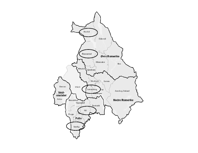
Figure 7: Meteorological stations where the precipitations in Section 5$\cdot$2 were recorded

References

- Aas et al. (2009) Aas, K., C. Czado, A. Frigessi, and H. Bakken (2009). Pair-copula constructions of multiple dependence. Insurance: Mathematics and Economics 44(2).
- Bedford and Cooke (2001) Bedford, T. and R. Cooke (2001). Probabilistic density decomposition for conditionally dependent random variables modeled by vines. Annals of mathematics and Artificial Intelligence 32, 245–268.
- Bedford and Cooke (2002) Bedford, T. and R. M. Cooke (2002). Vines—a new graphical model for dependent random variables. The Annals of Statistics 30(4), 1031–1068.
- Berg and Aas (2009) Berg, D. and K. Aas (2009). Models for construction of multivariate dependence. European Journal of Finance 15, 639–659.
- Brechmann et al. (2012) Brechmann, E. C., C. Czado, and K. Aas (2012). Truncated regular vines in high dimensions with application to financial data. Canadian Journal of Statistics xx, in press.
- Bücher and Dette (2010) Bücher, A. and H. Dette (2010). A note on bootstrap approximations for the empirical copula process. Statistics & Probability Letters 80(23-24), 1925–1932.
- Deheuvels (1979) Deheuvels, P. (1979). La fonction de dépendance empirique et ses propriétés. Bulletin de la Classe des Sciences, Académie Royale de Belgique 65, 274–292.
- Dissmann et al. (2011) Dissmann, J., E. Brechmann, C. Czado, and K. Kurowicka (2011). Selecting and estimating regular vine copulae and application to financial returns. Submitted for publication.
- Fermanian et al. (2004) Fermanian, J.-D., D. Radulović, and M. H. Wegkamp (2004). Weak convergence of empirical copula processes. Bernoulli 10, 847–860.
- Genest and Rémillard (2008) Genest, C. and Rémillard (2008). Validity of the parametric bootstrap for goodness-of-fit testing in semiparametric models, annales de iinstitut henri poincar´e. probabilit´es et statistiques 44 (in press)goodness-of-fit tests for copulas: a review and power study. Annales de I’Institut Henri Poincaré. Probabilités et Statistiques 44, 1096–1127.
- Genest et al. (2009) Genest, C., B. Rémillard, and D. Beaudoin (2009). Goodness-of-fit tests for copulas: a review and power study. Insurance: Mathematics and Economics 44, 199–213.
- Hobæk Haff (2012) Hobæk Haff, I. (2012). Parameter estimation for pair-copula constructions. Bernoulli xx, in press.
- Hobæk Haff et al. (2010) Hobæk Haff, I., K. Aas, and A. Frigessi (2010). On the simplified pair-copula construction – simply useful or too simplistic? Journal of Multivariate Analysis 101, 1296–1310.
- Joe (1996) Joe, H. (1996). Distributions with Fixed Marginals and Related Topics, Chapter Families of m-variate distributions with given margins and m(m-1)/2 dependence parameters, pp. 120–141. IMS, Hayward, CA.
- Kolbjørnsen and Stien (2008) Kolbjørnsen, O. and M. Stien (2008). D-vine creation of non-gaussian random field. In Procedings of the Eight International Geostatistics Congress, pp. 399–408. GECAMIN Ltd.
- Kurowicka and Cooke (2006) Kurowicka, D. and R. Cooke (2006). Uncertainty Analysis with High Dimensional Dependence Modelling. New York: Wiley.
- Min and Czado (2010) Min, A. and C. Czado (2010). Bayesian inference for multivariate copulas using pair-copula constructions. Journal of Financial Econometrics 8(4), 511–546.
- Min and Czado (2011) Min, A. and C. Czado (2011). Bayesian model selection for multivariate copulas using pair-copula constructions. Canadian Journal of Statistics 39(2), 239–258.
- Rémillard and Scaillet (2009) Rémillard, B. and O. Scaillet (2009). Testing for equality between two copulas. Journal of Multivariate Analysis 100(3), 377–386.
- Rüschendorf (1976) Rüschendorf, L. (1976). Asymptotic distributions of multivariate rank order statistics. The Annals of Statistics 4(5), 912–923.
- Segers (2012) Segers, J. (2012). Asymptotics of empirical copula processes under nonrestrictive smoothness assumptions. Bernoulli xx, to appear. arXiv:1012.2133 [math.ST].
- Stute (1984) Stute, W. (1984). The oscillation behavior of empirical processes: The multivariate case. AoP 12, 361–379.
- Tsukahara (2005) Tsukahara, H. (2005). Semiparametric estimation in copula models. CDA 33, 357–375.
- van der Vaart and Wellner (2007) van der Vaart, A. and J. A. Wellner (2007). Empirical processes indexed by estimated functions. In Asymptotics: Particles, Processes and Inverse Problems, Volume 55 of IMS Lecture Notes–Monograph Series, pp. 234–252. IMS.