A Multi-Wavelength Statistical Study of Supra-Arcade Downflows

Abstract

Sunward-flowing voids above post-coronal mass ejection flare arcades, also known as supra-arcade downflows (SADs), have characteristics consistent with post-reconnection magnetic flux tube cross-sections. Applying semi-automatic detection and analysis software to a large sample of flares using several instruments (e.g., Hinode/XRT, Yohkoh/SXT, TRACE, and SOHO/LASCO), we have estimated parameters such as speeds, sizes, heights, magnetic flux, and relaxation energy associated with SADs, which we interpret as reconnection outflows. We also present speed and height measurements of shrinking loops in comparison to the SAD observations. We briefly discuss these measurements and what impact they have on reconnection models.

Department of Physics, Montana State University, P.O. Box 173840, Bozeman, MT 59717-3840, USA

1 Introduction

Long duration flaring events are often associated with downflowing voids and/or loops in the supra-arcade region (see Fig. 1 for example images) whose theoretical origin as newly reconnected flux tubes has been supported by observations (McKenzie & Hudson 1999; McKenzie 2000; Innes et al. 2003; Asai et al. 2004; Sheeley et al. 2004; Khan et al. 2007; Reeves et al. 2008; McKenzie & Savage 2009; Savage et al. 2010).

The downflowing voids, or supra-arcade downflows (SADs; Fig 1a), differ in appearance from downflowing loops, or supra-arcade downflowing loops (SADLs; Fig. 1b); however, the explanation for this can be derived simply from observational perspective. If the loops are viewed nearly edge-on as they retract through a bright current sheet, then SADs may represent the cross-sections of the SADLs (see Figure 2). Since neither SADs nor SADLs can be observed 3-dimensionally by an independent imaging instrument, proving this hypothetical connection is not possible with a single image sequence. However, their general bulk properties, such as velocity, size, and magnetic flux, can be measured and should be comparable if this scenario is correct. Moreover, measuring these parameters for a large sample of SADs and SADLs yields constraints that are useful for development of numerical models/simulations of 3D magnetic reconnection in the coronae of active stars. We present analysis of flows from 35 flares and compare the results of general bulk properties, including magnetic flux and shrinkage energy estimates, from SADs and SADLs. These comparisons provide compelling evidence linking SADs to SADLs and constraints on flare magnetic reconnection models.

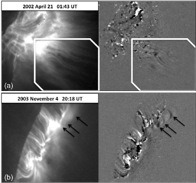
Figure 1.: (a) Example image from the April 21, 2002 TRACE flare showing supra-arcade downflows (SADs) enclosed within the white box. (b) Example image from the November 4, 2003 flare with supra-arcade downflowing loops (SADLs) indicated by the arrows. The left panel of each set is the original image. The right panel has been enhanced for motion via run-differencing and scaled for contrast.

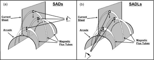
Figure 2.: (a) Cartoon depiction of supra-arcade downflows (SADs) resulting from 3D patchy reconnection. Discrete flux tubes are created, which then individually shrink, dipolarizing to form the post-eruption arcade. (b) Cartoon depiction of supra-arcade downflowing loops (SADLs) also resulting from 3D patchy reconnection. Note that the viewing angle, indicated by the eye position, is perpendicular to that of SADs observations.

2 Analysis

Considering the substantial uncertainty sources associated with flow detections, flow measurements should be taken as imprecise; however, the large number of fairly well-defined limb downflows (total of 369) tracked from our flare list make it possible to consider ranges and trends in the data.

2.1 Synthesis of Frequency Diagrams

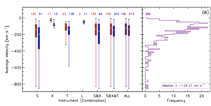
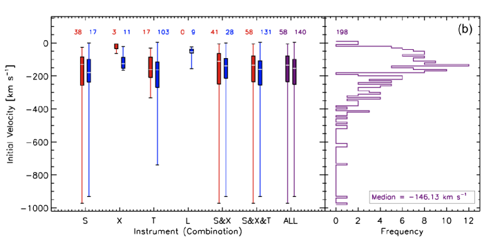
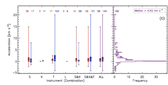
Figure 3.: Synthesis of the de-projected trajectory parameter estimates. (a) De-projected average velocity. (b) De-projected initial velocity. (c) De-projected acceleration. (Refer to the text for a detailed description of these figures.)

Figures 3, 4, and 5 synthesize the flow measurement results from all of the flares under consideration. Each plot in the figures consists of a quartile plot in the left panel and a histogram in the right. For the quartile plots, the measurement is plotted against the instrument (or instrument combination) being considered (S: SXT; X: XRT; T: TRACE; L: LASCO; All: S&X&T&L). For Figs. 3 and 4, the left (red or purple) box-and-whisker range per instrument (or instrument combination) represents SADs measurements while the right (blue or purple) one represents SADLs measurements. For Fig. 5, the east (pink or green) and west (olive or green) limbs are compared instead of SADs to SADLs. The lines (or whiskers) extending from the boxes indicate the full range of the data. The boxes span the range of the middle 50% of the data. The (white) line through the box indicates the median of the data. Along the top of these plots, the number of flows used to derive the associated measurements is labeled. The combination of the data in the final two (purple or green) box-and-whisker plots is contained within the histogram panel. The median of the histogram is displayed in the legend.

LASCO measurements are not included in Figs. 4 or 5 since its resolution (11.4 arcsec/pix) is so much poorer and its observational regime high above the limb ($>$ 2.5 R_⊙ for C2) is so very different from that of the other instruments, making comparisons more complicated. Deriving magnetic fields at such heights is not applicable with our method either plus determining precise footpoints without coincidental data from other instruments is nearly impossible. The total number of flows under consideration after removing those observed by LASCO is 358.

2.1.1 Velocity and Acceleration

There is general agreement between SADs and SADLs, the instruments, and the SXR versus EUV bandpasses for the average velocity, initial velocity, and acceleration measurements (Figure 3). Note that the initial velocity and acceleration plots do not incorporate all 369 available flows. Instead, only those flows tracked in at least 5 frames were included because these measurements rely on fitting the trajectories to a 2D polynomial fit. Using fewer than 5 points leads to unreliable results. Also note that a positive downflow acceleration means that the flow is slowing.

2.1.2 Area

A strong correspondence between instrument resolution (SXT: 2.5–4.9 arcsec/pix; XRT: 1 arcsec/pix; TRACE: 0.5 arcsec/pix) and measured area is shown in the initial area quartile plot (Figure 4a). The SADLs and XRT SADs area measurements are very strongly peaked due to their manual assignments (versus threshold detection)—hence the lack of distinct quartiles.

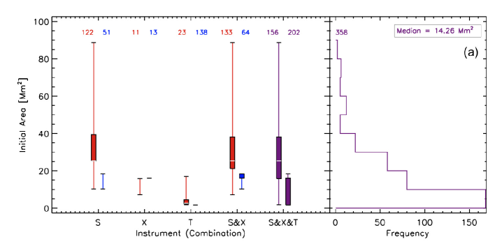
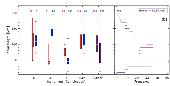
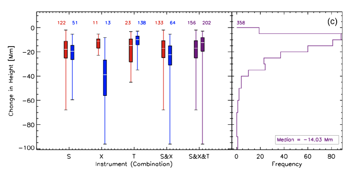
Figure 4.: Synthesis of the area and height parameter estimates. (a) Initial area. (b) De-projected initial height. (c) De-projected change in height. (Refer to the text for a detailed description of these figures).

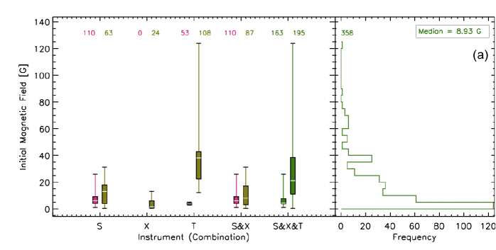
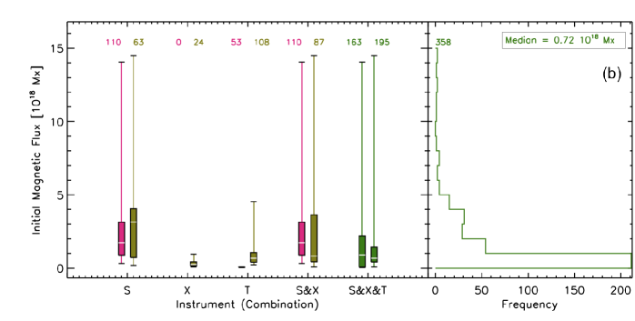
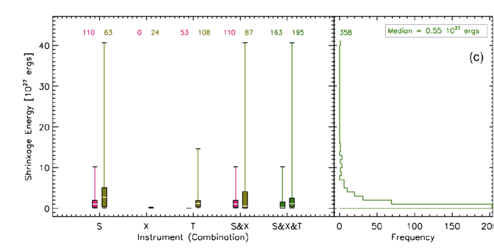
Figure 5.: Synthesis of the magnetic parameter estimates (a) Initial magnetic field. (b) Initial magnetic flux. (c) Shrinkage energy. (Refer to the text for a detailed description of these figures).

2.1.3 Height

The initial height ranges (Fig. 4b) show decent agreement between the ranges; however, there is a fair amount of scatter in the medians which requires more detailed understanding of the analyzed flares to explain. The initial heights for both SADs and SADLs observed by SXT offer very good agreement. XRT observations, while agreeing with SXT’s range of initial heights, show no agreement between SADs and SADLs. This discrepancy is due to a combination of factors: (1) XRT has observed very few SADs as yet; (2) XRT observations are rarely sufficiently exposed to illuminate the supra-arcade region; therefore, XRT SADs have only been observed nearer to the solar surface; (3) The SADLs observed by XRT are derived from the “Cartwheel CME” flare (Savage et al. 2010) during which the footpoints were obscured by the limb enabling very long exposure durations. In fact, a disconnection event associated with this flare (Savage et al. (2010), Sect. 3.2 therein) was observed at nearly 190 Mm above the solar surface, which is at the maximum of the combined instrument ranges. TRACE’s temperature coverage targets plasma on order of 1 MK with some overlap in the 11–26 MK range with the SXR imagers. The image exposure durations are also optimized to observe the flaring region near the solar surface. Consequently, the observed initial heights of SADs and SADLs measured with TRACE are limited to the region near the top of the growing post-eruption arcade where the hot plasma in the current sheet is most illuminated. This results in initial heights lower than many of those reported for SXT and XRT.

The change in heights shown in Fig. 4c are naturally flare and field of view (FOV) dependent. Even so, there is general agreement between SADs, SADLs, and instrument except for XRT. The explanation for this XRT discrepancy is the same as that for the initial height XRT discrepancy described above (i.e., the flows for the “Cartwheel CME” flare could be tracked further through the FOV).

2.1.4 Magnetic Measurements

Figure 5a is provided as a visual reference for the initial magnetic fields which are used to calculate the magnetic flux ($\Phi=B\times A$, Fig. 5b) and the shrinkage energy ($\Delta W=B^{2}A\Delta L/8\pi$, Fig. 5c). Refer to McKenzie & Savage (2009), Sect. 4.5, for a detailed description of the shrinkage energy calculations. The initial magnetic field estimates for the TRACE flares are larger than the majority of those from SXT and XRT because (1) the TRACE flares analyzed are highly energetic according to their GOES classifications and (2) the flows are observed closer to the surface (see Fig. 4b) where the magnetic field is stronger according to the PFSS model (Schatten et al. 1969; Schrijver & De Rosa 2003). East and west limb measurements are compared in Fig. 5 to show the effect of using less reliable east-limb magnetograms. The tendency for west limb flares to have stronger initial magnetic field estimates is noticeable in Fig. 5a and carries through into the initial magnetic flux and shrinkage energy plots (Figs. 5b and 5c, respectively). The dichotomy is most noticeable in the shrinkage energy estimates due to the $B^{2}$ component.

2.2 Discussion

Interpreting SADs as the cross-sections of retracting reconnected flux tubes also means that if they are viewed from an angle that is not near perpendicular to the arcade axis (i.e., the polarity inversion line), the downflows will instead appear as shrinking loops. These shrinking loops (SADLs) have indeed been clearly observed with all of the instruments under investigation. Therefore, comparing observations of SADs to those of SADLs can help to support or refute the SADs hypothesis.

Figures 3 through 5 present a summary of the instrument and SAD/SADL comparisons. These figures show that the flow velocities and accelerations agree between the instruments quite well. Height measurements agree except for those measured with XRT due to the exceptional flow heights observed for the “Cartwheel CME” flare (Savage et al. 2010). Figure 4a shows that the area measurements are understandably resolution dependent, which indicates that we may not be able to observe the smallest loop sizes. The flux and energy measurements are area dependent and therefore instrument dependent. There is also a limb dependence with the magnetic measurements due to the use of modeling based on magnetograms. Even so, there is decent agreement between all of the instruments (LASCO is only included with the velocity and acceleration comparisons as explained in Section 2.1). Beyond the agreement between the SADs and SADLs measurements, the high-resolution TRACE observations clearly show both SADs and SADLs occurring during the same flare depending on the arcade viewing angle which curves within the active region.

The measured cross-sectional areas range from $\sim$2 to 90 Mm², with at least 75% being smaller than 40 Mm² (Figure 4a). The flows typically move at speeds on order of 10² km s^-1 with accelerations that are near zero or slightly decelerating. The most complete flow paths show significant deceleration near the top of the arcade. There is a range of initial heights depending on the quality of the image set, but they are generally about 10⁵ km above the solar surface with a path length of $\sim$10⁴ km. Each tube carries $\sim$10¹⁸ Mx of flux and releases on order of 10²⁷ ergs of energy as it retracts. A lower limit of 10¹⁶ Mx s^-1 can be put on the reconnection rate by considering the total flux released by the observed flows for 5 flares from our list.

The observational findings presented here provide a more complete description of the SAD/SADL phenomenon than has previously been available. Assuming that SADs and SADLs are thin, post-reconnection loops based on this body of evidence, the measurements obtained through this analysis and summarized above provide useful constraints for reconnection models. Area estimates can constrain the diffusion time per episode and reconnection rates can be derived to distinguish between fast and slow reconnection. Creation of outflowing flux tubes carrying on order of 10¹⁸ Mx of flux, with net reconnection rates of at least 10¹⁶ Mx s^-1, should be an objective of realistic models of 3D reconnection. The lack of acceleration of the downflow speeds and their discrete nature tends to favor 3D patchy Petschek reconnection. Speeds almost an order of magnitude slower than traditionally assumed Alfvén speeds are an unexpected consequence of the flow measurements; therefore, analyzing the effect of some source of drag on the downflow trajectories using models (an effort begun by Linton & Longcope 2006) could provide valuable insight into this discrepancy.

Acknowledgments

This work was supported by NASA grant NNM07AB07C. SLS is grateful for the meeting registration support provided by the Hinode-4 SOC.

References

- Asai et al. (2004) Asai, A., Yokoyama, T., Shimojo, M., & Shibata, K. 2004, ApJ, 605, L77
- Innes et al. (2003) Innes, D. E., McKenzie, D. E., & Wang, T. 2003, Solar Phys., 217, 247
- Khan et al. (2007) Khan, J. I., Bain, H. M., & Fletcher, L. 2007, A&A, 475, 333
- Linton & Longcope (2006) Linton, M. G., & Longcope, D. W. 2006, ApJ, 642, 1177
- McKenzie (2000) McKenzie, D. E. 2000, Solar Phys., 195, 381
- McKenzie & Hudson (1999) McKenzie, D. E., & Hudson, H. S. 1999, ApJ, 519, L93
- McKenzie & Savage (2009) McKenzie, D. E., & Savage, S. L. 2009, ApJ, 697, 1569
- Reeves et al. (2008) Reeves, K. K., Seaton, D. B., & Forbes, T. G. 2008, ApJ, 675, 868
- Savage et al. (2010) Savage, S. L., McKenzie, D. E., Reeves, K. K., Forbes, T. G., & Longcope, D. W. 2010, ApJ, 722, 329
- Schatten et al. (1969) Schatten, K. H., Wilcox, J. M., & Ness, N. F. 1969, Solar Phys., 6, 442
- Schrijver & De Rosa (2003) Schrijver, C. J., & De Rosa, M. L. 2003, Solar Phys., 212, 165
- Sheeley et al. (2004) Sheeley, N. R., Jr., Warren, H. P., & Wang, Y.-M. 2004, ApJ, 616, 1224