Ab initio quantum dynamics using coupled-cluster

Abstract

The curse of dimensionality (COD) limits the current state-of-the-art ab initio propagation methods for non-relativistic quantum mechanics to relatively few particles. For stationary structure calculations, the coupled-cluster (CC) method overcomes the COD in the sense that the method scales polynomially with the number of particles while still being size-consistent and extensive. We generalize the CC method to the time domain while allowing the single-particle functions to vary in an adaptive fashion as well, thereby creating a highly flexible, polynomially scaling approximation to the time-dependent Schrödinger equation. The method inherits size-consistency and extensivity from the CC method. The method is dubbed orbital-adaptive time-dependent coupled-cluster (OATDCC), and is a hierarchy of approximations to the now standard multi-configurational time-dependent Hartree method for fermions. A numerical experiment is also given.

I Introduction

Presently, the most advanced ab initio approximations to the time-dependent Schrödinger equation for a system of identical particles are the multiconfigurational time-dependent Hartree methods for fermions (MCTDHF) and variants [1, 2, 3]. These methods apply the time-dependent variational principle [4, 5, 6] to an $N$-body wavefunction ansatz being a Slater determinant expansion using a finite (incomplete) set of $L\geq N$ orbitals $\varphi_{p}$ with creation operators $c^{\dagger}_{p}$ (with $\{c_{p},c^{\dagger}_{q}\}=\delta_{pq}$ for fermions),

$$|\Psi_{\text{MCTDHF}}\rangle\equiv\sum_{p_{1}}\sum_{p_{2}>p_{1}}\cdots\sum_{p_{N}>p_{N-1}}A_{p_{1}\cdots p_{N}}c^{\dagger}_{p_{1}}c^{\dagger}_{p_{2}}\cdots c^{\dagger}_{p_{N}}|-\rangle,$$

where both the amplitudes $A_{p_{1}\cdots p_{N}}$ and the orbitals $\varphi_{p}$ are free to vary in single-particle space. Varying the orbitals in this way is especially important if studies of unbound systems are desired, such as the study of ionization of atoms or molecules. The key point is that, if the orbitals are not optimized, a system in the continuum would need a huge fixed basis. Moreover, the variational determination of the orbitals compresses the wavefunction in a quasi-optimal way: from time $t$ to $t+dt$, the basis is changed as so to minimize the $L^{2}$ norm error of the wavefunction [6].

While powerful, MCTDHF still suffers from exponential scaling of computational complexity with respect to the number of particles $N$ present; the somewhat prosaically termed “curse of dimensionality” (COD). The effect of the variational determination of the single-particle functions can be said to be a postponing of the COD to higher particle numbers. For example, for the simple time-dependent Hartree–Fock method (TDHF), i.e., MCTDHF using precisely $L=N$ orbitals and therefore only a single determinant $|\phi\rangle$, qualitatively good results may be achieved, even if the system is unbound [7].

One may attempt at reducing the exponential scaling by truncating the Slater determinant expansion at, say, single and double excitations relative to one of the determinants $|\phi\rangle=c^{\dagger}_{1}\cdots c^{\dagger}_{N}|-\rangle$, considered as a “reference determinant”,

$$|\Psi_{\text{MCTDHF-SD}}\rangle=\left(1+\sum_{ia}A_{i}^{a}c^{\dagger}_{a}c_{i}|\phi\rangle+\frac{1}{2!^{2}}\sum_{ijab}A_{ij}^{ab}c^{\dagger}_{a}c_{i}c^{\dagger}_{b}c_{j}\right)|\phi\rangle\equiv(1+A_{SD})|\phi\rangle,$$ (1)

hoping that the higher-order excited determinants’ contribution can be neglected. (We have arbitrarily chosen intermediate normalization $\langle\phi|\Psi\rangle=1$. In the sums, $i,j\leq N$ and $a,b>N$ is assumed.) This would achieve polynomial scaling but would destroy the important property of size-consistency [8, 9]: approximation of non-interacting subsystems separately at the singles and doubles level would not be consistent with approximating the whole at the same level; independent excitations of the subsystems are neglected, giving rise to artificial correlation effects.

In this article, we develop a time-dependent version of the popular coupled-cluster (CC) method for fermions, where we allow the orbitals to vary in a similar fashion to MCTDHF. We call the method orbital adaptive time-dependent coupled-cluster (OATDCC). Formally, the two methods are very similar, with closely related equations of motion. The main difference is the fact that coupled-cluster is not variational in the usual sense, rather, it is naturally cast in a bivariational setting, a generalization of the variational approach [10]. Bivariational functionals are complex analytic, while the standard variational functionals are manifestly real. Moreover, approximations of both the wavefunction $|\Psi\rangle$ the complex conjugate $\langle\Psi|$ must be introduced. For the version of CC that has now become standard (referred to as “standard CC” in this paper), the wavefunctions in the singles and double approximation (CCSD) are parametrized according to

$$|\Psi_{\text{CC}}\rangle \equiv e^{T}|\phi\rangle,\quad T=\sum_{ai}\tau_{i}^{a}c^{\dagger}_{a}\tilde{c}_{i}+\frac{1}{2!^{2}}\sum_{ijab}\tau_{ij}^{ab}c^{\dagger}_{a}\tilde{c}_{i}c^{\dagger}_{b}\tilde{c}_{j}+\cdots$$ (2a)

$$\langle\tilde{\Psi}_{\text{CC}}| \equiv\langle\tilde{\phi}|(1+\Lambda)e^{-T},\quad\Lambda=\sum_{ai}\lambda_{a}^{i}c^{\dagger}_{i}\tilde{c}_{a}+\frac{1}{2!^{2}}\sum_{ijab}\lambda_{ab}^{ij}c^{\dagger}_{i}\tilde{c}_{a}c^{\dagger}_{j}\tilde{c}_{b}+\cdots$$ (2b)

where $\langle\tilde{\Psi}_{\text{CC}}|$ approximates $\langle\Psi|/\langle\Psi|\Psi\rangle$. The operator $T$ is called a cluster operator and produces excitations with respect to a reference Slater determinant $|\phi\rangle$. The amplitudes $\tau_{i}^{a}$ and $\tau_{ij}^{ab}$ correspond (to first order) to the expansion coefficients $A_{i}^{a}$ and $A_{ij}^{ab}$ of Eqn. (1). The cluster operator $\Lambda$ is a de-excitation operator, and its amplitudes $\lambda_{a}^{i}$ and $\lambda_{ab}^{ij}$ are essentially the parameters of $\langle\tilde{\Psi}_{\text{CC}}|$, which also is composed of excitations relative to a reference bra determinant $\langle\tilde{\phi}|$. To anticipate the developments in later sections, we have introduced creation and annihilation operators with respect to biorthogonal orbitals $\varphi_{p}$ and $\tilde{\varphi}_{q}$, i.e.,

$$\left\{\tilde{c}_{p},c^{\dagger}_{q}\right\}=\tilde{c}_{p}c^{\dagger}_{q}+c^{\dagger}_{q}\tilde{c}_{p}\equiv\langle\tilde{\varphi}_{p}|\varphi_{q}\rangle,$$

That is to say, $|\Psi\rangle$ is built using the $\varphi_{p}$, while $\langle\tilde{\Psi}|$ is built using $\tilde{\varphi}_{p}$. This relaxation of orthonormality of the orbitals is necessary to ensure that the bivariational functional is complex analytic if the orbitals are to be treated as variational parameters, as discussed in Section II.2.

Our treatment can be viewed as a generalization of the standard CC Lagrangian approach to linear response theory [11, 10, 12, 13], where the $\Lambda$ amplitudes are time-dependent Lagrangian multipliers as introduced in a constrained minimization of the CC energy. However, we emphasize the bivariational point of view, where $\Lambda$ becomes a part of the wave function parametrization. In Ref. [14] even biorthogonal orbitals were consideres.

For an excellent introduction to CC theory, see the article [15] by Crawford, and the review [16] by Bartlett and Musiał, as well as the textbooks [9] by Shavitt and Bartlett and [17] by Harris et al. For the present work, the article [10] is fundamental, as it casts the CC theory in the bivariational framework, an approach not emphasized in most introductions to CC theory.

The OATDCC method considers the standard CC ansatz plugged into the proper bivariational functional, see Section III.4 below. In addition to having the $T$ and $\Lambda$ amplitudes as degrees of freedom, the orbitals $|\varphi_{p}\rangle$ and approximations $\langle\tilde{\varphi}_{p}|$ to their complex conjugates are varied. It turns out the relaxation of the orbitals makes the singles amplitudes $\tau_{i}^{a}$ and $\lambda_{a}^{i}$ redundant. Truncation of the remaining terms at doubles, triples, etc, then gives a hierarchy of approximations with TDHF at one end ($T=\Lambda=0$), and full MCTDHF (no truncation of $T$ or $\Lambda$) at the other. Inbetween we have the doubles approximation (OATDCCD), doubles-and-triples approximation (OATDCCDT), and so on. Considering the success of the CC method for structure calculations and the MCTDHF method for dynamics, OATDCC should be a viable alternative to MCTDHF with asymptotically much lower cost but good accuracy. Importantly, OATDCC is size-consistent.

There are few applications of CC methods to ab initio dynamics in the literature. It was, however, proposed as early as 1978 by Schönhammer and Gunnarsson [18], and independently by Hoodbhoy and Negele [19, 20], who even considered time-dependent orbitals, albeit with an explicit time-dependence. We shall discuss their approach briefly in Section V.1. Recently, the standard CC ansatz using a fixed basis was applied to laser-driven dynamics of some small molecules [21], but with expectation values calculated in a different way from the usual CC approach.

This article is written with the MCTDHF community in mind. Since bivariational principles are rarely considered (which is true for the CC community as well), we give a somewhat detailed discussion in Section II. As CC theory might be unfamiliar, and as we use a somewhat unfamiliar variational approach to derive CC theory, Section III is devoted to the basics of the CC formalism, leading up to the case where the orbitals are varied freely. In Section IV we discuss the OATDCC functional and derive the corresponding equations of motion. We then perform a simple numerical experiment in Section VI to demonstrate the method before we conclude the paper.

CC calculations invariably involve a lot of algebra. Therefore, in A, algebraic expressions for various quantities appearing in the OATDCCD method are listed. These are generated using symbolic algebra software developed with the SymPy library for the programming language Python [22]. An independent derivation of MCTDHF is given in B in order to shed further light on the connections between the variational and the bivariational principles. It may also serve as a helpful device for the researchers in the audience not familiar with MCTDHF theory.

No attempt is made to be mathematically rigorous in this article, as like the standard CC method [23, 24, 25] and the MCTDHF method [6, 26, 27, 28] such an analysis is expected to be quite involved. Instead, we make formal computations as if all operators present were bounded or the spaces finite dimensional.

II Bivariational principles

II.1 Functionals

Let $A$ be an operator over Hilbert space $\mathcal{H}$, and consider the functional

$$\mathcal{E}_{A}:\mathcal{H}^{\prime}\times\mathcal{H}\longrightarrow\mathbb{C},\quad\mathcal{E}_{A}[\langle\Psi^{\prime}|,|\Psi\rangle]\equiv\frac{\langle\Psi^{\prime}|A|\Psi\rangle}{\langle\Psi^{\prime}|\Psi\rangle}$$

defined whenever the expression makes sense. Note that the arguments are two independent Hilbert space elements. The functional $\mathcal{E}_{A}$ is a generalization of the expectation value functional to operators that are not necessarily Hermitian, and for obvious reasons it may be called the bivariational expectation value functional [10, 29]. Consider the conditions for vanishing first variation, $\delta\mathcal{E}_{A}=0$, for all independent variations of $\langle\Psi^{\prime}|$ and $|\Psi\rangle$. A straightforward formal calculation gives the stationary conditions

$$(A-a)|\Psi\rangle=0\quad\text{and}\quad\langle\Psi^{\prime}|(A-a)=0,$$ (3)

with

$$a=\mathcal{E}_{A}[\langle\Psi^{\prime}|,|\Psi\rangle]$$

being the value of $\mathcal{E}_{A}$ at the critical point. In other words $\langle\Psi^{\prime}|$ and $|\Psi\rangle$ with $\langle\Psi^{\prime}|\Psi\rangle\neq 0$ are left- and right eigenvectors, respectively, of the operator $A$, with eigenvalue $a$. Computing the eigenvalues and eigenvectors from $\delta\mathcal{E}_{A}=0$ is therefore referred to as “the bivariational principle.”

Since the system Hamiltonian $H=H^{\dagger}$ is the generator for the time-evolution of the system, we consider the following bivariational generalization of the usual action functional [10, 5], i.e.,

$$\mathcal{S}[\langle\Psi^{\prime}|,|\Psi\rangle] \equiv\int_{0}^{T}\frac{\langle\Psi^{\prime}(t)|\left(\mathrm{i}\hbar\frac{\partial}{\partial t}-H\right)|\Psi(t)\rangle}{\langle\Psi^{\prime}(t)|\Psi(t)\rangle}\;\mathrm{d}t$$

$$=\int_{0}^{T}\mathrm{i}\hbar\frac{\langle\Psi^{\prime}(t)|\frac{\partial}{\partial t}\Psi(t)\rangle}{\langle\Psi^{\prime}(t)|\Psi(t)\rangle}-\mathcal{E}_{H}[\langle\Psi^{\prime}(t)|,|\Psi(t)\rangle]\;\mathrm{d}t,$$ (4)

where it is understood that the functional depends on the whole history of the system from time $t=0$ to $t=T$. Suppose $\mathcal{S}$ is stationary ($\delta\mathcal{S}=0$) under all variations of $\langle\Psi^{\prime}|$ and $|\Psi\rangle$ vanishing at the endpoints $t=0,T$. Straightforward manipulations now give, up to irrelevant time-dependent phase constants,

$$\mathrm{i}\hbar\frac{\partial}{\partial t}|\Psi(t)\rangle=H|\Psi(t)\rangle\quad\text{and}\quad-\mathrm{i}\hbar\frac{\partial}{\partial t}\langle\Psi^{\prime}(t)|=\langle\Psi^{\prime}(t)|H.$$ (5)

Consequently, we note that the time-dependent Schrödinger equation and its complex conjugate arise from a time-dependent bivariational principle.

In both the stationary and time-dependent case, it is convenient to do a reparametrization $\langle\tilde{\Psi}|=\langle\Psi^{\prime}|\Psi\rangle^{-1}\langle\Psi^{\prime}|$ so that

$$\langle\tilde{\Psi}|\Psi\rangle=1,$$ (6)

eliminating the denominator in each functional. For the stationary case, this effectively eliminates one of the two eigenvalue equations (3), and makes $\langle\tilde{\Psi}|$ a unique function of $|\Psi\rangle$ and vice versa. To see this, note that since (a) eigenvectors corresponding to different eigenvalues are always orthogonal, and since (b) $\langle\tilde{\Psi}|\Psi\rangle=1$, $\langle\tilde{\Psi}|$ is uniquely given by $|\Psi\rangle$ at the critical point as the biorthogonal left eigenvector corresponding to the right eigenvector $|\Psi\rangle$.

For the time-dependent case, the normalization $\langle\tilde{\Psi}(t)|\Psi(t)\rangle=1$ eliminates one of the Schrödinger equations (5), but the phase ambiguity is still present for the remaining equation, a similar situation as the stationary case.

Unless otherwise stated, the normalization (6) is assumed in the following, and it is indicated by the tilde $\langle\tilde{\Psi}|$ instead of the prime $\langle\Psi^{\prime}|$.

It is also natural to assume some secondary normalization on $|\Psi\rangle$, such that the critical point actually becomes locally unique for both the time-dependent and time-independent cases. (“Locally unique” means that there may be many critical points but that they are isolated.) This is done in CC theory, where $\langle\tilde{\phi}|\Psi\rangle=1$ is assumed. This removes phase ambiguity in both time-dependent and time-independent pictures.

II.2 Generating approximations from submanifolds

Contrary to the usual variational principles, in the bivariational principles the wavefunction and its complex conjugate are formally independent. When applied to Hermitian operators this opens up possibilities for more general approximations compared to the standard variational principles to spectra and dynamics, when the variations are restricted to some predefined approximation manifold. However, where the usual “Hermitian” time-dependent variational principle is, to paraphrase Kramer and Saraceno [5], a deaf and dumb procedure that always gives an answer, the bivariational principle requires a more careful approach, as we will discuss in this section.

Perhaps for this reason, the bivariational principles are little known. The author has found only a few relevant sources in the literature apart from Arponen’s seminal coupled-cluster paper [10], the most relevant ones being a brief mention by Killingbeck in his review on perturbation theory [30] and a discussion by Löwdin et al. [29] concerning self-consistent field-calculations on non-Hermitian (complex scaled) Hamiltonians. The bivariational principle seems largely unexplored.

It is important to note that the standard critique of coupled-cluster is that it is “non-variational”. While it is true that it makes estimation of errors harder, it is not a serious drawback in any other sense, since the calculation is firmly rooted in a variational principle. For example, if $H$ does not depend explicitly on time, $(d/dt)\mathcal{E}_{H}\equiv 0$, i.e., energy is conserved. Probability is always conserved, $(d/dt)\mathcal{E}_{1}=(d/dt)\langle\tilde{\Psi}|\Psi\rangle\equiv 0$. Just like the usual time-dependent variational principle, these are simple consequences of the symmetries of the action functional.

For bivariational approximations, one introduces different parametrizations of the wavefunction $|\Psi\rangle$ and its complex conjugate $\langle\Psi|$, which is contrary to the usual variational principle. Notice that in Eqn. (2), different parametrizations $|\Psi_{\text{CC}}\rangle$ and $\langle\tilde{\Psi}_{\text{CC}}|$ are used, but $\langle\tilde{\Psi}_{\text{CC}}|\Psi_{\text{CC}}\rangle=1$. Formally, we do a variation over a manifold $\mathcal{M}\subset\mathcal{H}^{\prime}\times\mathcal{H}$, i.e., $(\langle\tilde{\Psi}|,|\Psi\rangle)\in\mathcal{M}$. Alternatively, one may think of $\mathcal{M}$ as a subset of rank-one density operators $u=|\tilde{\Psi}\rangle\langle\Psi|$, $\operatorname{Tr}(u)=1$, where $u^{\dagger}\neq u$ is allowed.

As $\mathcal{H}$ is a complex space, the functionals $\mathcal{E}_{H}$ and $\mathcal{S}$ are complex. On the other hand, in the usual variational principle, the functionals are always real-valued. This has some interesting consequences. We now briefly discuss four important aspects: the analytic structure of the functionals, the need for systematic refinability of $\mathcal{M}$, interpretations of complex critical points, and even-dimensionality of $\mathcal{M}$.

The parametrization of $u=(\langle\tilde{\Psi}|,|\Psi\rangle)$ must be complex analytic, at least locally. A parametrization which is not analytic is, in essence, a real parametrization, since it depends on both the real and imaginary parts of the (local) coordinates $z\in\mathbb{C}^{n}$ separately, and not only $\operatorname{Re}z+\mathrm{i}\operatorname{Im}z$. Thus, we have $2n$ real coordinates. Since both $\operatorname{Re}\delta\mathcal{S}$ and $\operatorname{Im}\delta\mathcal{S}$ must vanish, this leads to $4n$ equations. Unless there is some extra structure, i.e., that $\operatorname{Im}\mathcal{S}\equiv 0$ such as in the standard variational principle, a solution cannot be expected to exist. Correspondingly, the bivariational functionals should be complex analytic. Nowhere should explicitly real parameters occur, and nowhere should parameters be explicitly complex conjugated.

Suppose the system Hamiltonian $H$ is bounded from below, i.e., the expectation value is bounded from below. This is the source of the usefulness of the Hermitian stationary variational principle, since any parametrization gives an upper bound for the ground state energy. A potential danger with the bivariational expectation value functional is that it is not bounded from below, even if $H$ is. Indeed, $\mathcal{E}_{H}$ is complex analytic and can take on values in the whole of $\mathbb{C}$. One cannot insert “just anything” and hope to get sensible results by computing critical points. To avoid this problem, and to allow for the computation of error estimates, $\mathcal{M}$ should be chosen in a way that is in some sense systematically refinable towards the full space $\mathcal{H}^{\prime}\times\mathcal{H}$, e.g., there is some discretization parameter that can be used to measure the accuracy. In CC theory, this parameter is the truncation level of the cluster operators and the number $L$ of orbitals used.

Critical values of $\mathcal{E}_{H}$ for $H=H^{\dagger}$ may be complex, even though the exact eigenvalues are always real. However, if $H=H^{\dagger}$, the imaginary values of the critical values generally “should be small” if $\mathcal{M}$ is chosen “well enough”, and may correspondingly be ignored in order to assign a physical interpretation to the critical value, i.e., energy. This is also justified by the fact that the functional $\operatorname{Re}\mathcal{E}_{H}$ has the same critical points as $\mathcal{E}_{H}$ if the parametrization is analytic.

For the approximate manifold $\mathcal{M}$, we must be certain that the critical point $(\langle\tilde{\Psi}|,|\Psi\rangle)$ is locally unique. In particular, this is necessary for the corresponding critical value, i.e., $\mathcal{E}_{A}[\langle\tilde{\Psi}||\Psi\rangle]$, to be unique for any observable $A$. Otherwise, the physical state cannot be said to be well-defined. Intuitively, the parameters must then come in pairs; roughly stated every parameter in $|\Psi\rangle$ should have a parameter in $\langle\tilde{\Psi}|$.

This can be shown explicitly. Suppose $\langle\tilde{\Psi}|$ and $|\Psi\rangle$ are parametrized locally using some set of complex variables $z(t)=\mathbb{C}^{n}$, i.e., we have an approximating manifold $\mathcal{M}\subset\mathcal{H}^{\prime}\times\mathcal{H}$ whose dimension is assumed to be finite for simplicity. When inserted into the time-dependent bivariational functional, we obtain a new functional $F[z(\cdot)]=\mathcal{S}[\langle\tilde{\Psi}(z(\cdot))|,|\Psi(z(\cdot))\rangle]$, whose stationary point is given by the solution of the differential equation

$$\mathrm{i}\hbar C(z)\dot{z}=\nabla_{z}E(z),\quad E(z)=\mathcal{E}_{H}[\langle\tilde{\Psi}(z)|,|\Psi(z)\rangle].$$ (7)

The matrix $C(z)$ is given by

$$C(z)_{jk}=\Bigg{\langle}{\frac{\partial\tilde{\Psi}}{\partial z_{j}}\Bigg{|}\frac{\partial\Psi}{\partial z_{k}}}\Bigg{\rangle}-\Bigg{\langle}{\frac{\partial\tilde{\Psi}}{\partial z_{k}}\Bigg{|}\frac{\partial\Psi}{\partial z_{j}}}\Bigg{\rangle},$$

which is complex anti-symmetric. For any anti-symmetric matrix, if $\lambda$ is an eigenvalue of multiplicity $m$, so is $-\lambda$, implying that $C(z)$ is not invertible if $n$ is odd, since it must have a zero eigenvalue. Consequently, the approximation manifold must be complex even dimensional if Equation (7) is to have a unique solution.

III Coupled-cluster functionals

III.1 Biorthogonality of orbitals

The fact that we require our bivariational functionals to be analytic is important, as it necessitates the relaxation of the orthonormality the orbitals $\varphi_{p}$ by introducing a second set of biorthogonal orbitals $\tilde{\varphi}_{q}$, being in effect approximate complex conjugates of each other. However, they are introduced as independent complex parameters.

Consider a subspace $\mathcal{V}\subset\mathcal{H}$, generated by a finite set of orbitals $\Phi=(\varphi_{1},\varphi_{2},\cdots,\varphi_{L})$, which we write $\mathcal{V}=\mathcal{V}[\Phi]$. (We interpret $\varphi_{p}$ as the $p$th column of the matrix $\Phi$.) These orbitals need not be orthonormal; it is only the one-body space spanned by the $\varphi_{p}$ that matters. In the bivariational functionals, we desire to vary $\langle\tilde{\Psi}|$ in as large space $\tilde{\mathcal{V}}\subset\mathcal{H}^{\dagger}$ as possible, while guaranteeing the existence of a dual vector non-orthogonal to $|\Psi\rangle\in\mathcal{V}$. (Otherwise, the denominator in Eqn. (4) may vanish.) The only restriction on the space $\tilde{\mathcal{V}}$ is that it is generated by a set of dual orbitals $\tilde{\Phi}=(\tilde{\varphi}_{1};\cdots;\tilde{\varphi}_{L})$ (where we interpret $\tilde{\varphi}_{p}$ as the $p$th row of $\tilde{\Phi}$). Sometimes we will stress the fact that $\varphi_{p}$ and $\tilde{\varphi}_{p}$ are single-particle ket and bra-functions, respectively, by explicitly writing $|\varphi_{p}\rangle$ and $\langle\tilde{\varphi}_{p}|$.

Consider the overlap matrix $S$ with matrix elements $S_{pq}=\langle\tilde{\varphi}_{p}|\varphi_{q}\rangle$. Since the spaces $\mathcal{V}[\Phi]$ and $\tilde{\mathcal{V}}[\tilde{\Phi}]$ only depend on the subspaces spanned by $\Phi$ and $\tilde{\Phi}$, respectively, we may via a suitable transform assume that $S$ is diagonal with only $1$s and $0$s on the diagonal. If $S$ is invertible, then the orbitals are biorthogonal,

$$\langle\tilde{\varphi}_{p}|\varphi_{q}\rangle=\delta_{pq}.$$

It is straightforward to show the following claim: the existence of a $\langle\tilde{\Psi}|\in\tilde{\mathcal{V}}[\tilde{\Phi}]$ for every $|\Psi\rangle\in\mathcal{V}[\Phi]$ such that $\langle\tilde{\Psi}|\Psi\rangle\neq 0$ is equivalent to requiring the overlap matrix $S_{pq}=\langle\tilde{\varphi}_{p}|\varphi_{q}\rangle$ to be invertible, i.e., that the orbitals are biorthogonal. (A corresponding claim where the roles of $|\Psi\rangle$ and $\langle\tilde{\Psi}|$ are reversed is equivalent.)

Biorthogonality is equivalent to

$$\langle\tilde{\phi}_{p_{1}\cdots p_{N}}|\phi_{q_{1},\cdots,q_{N}}\rangle=\delta_{p_{1},q_{1}}\cdots\delta_{p_{N},q_{N}}$$

for the Slater determinant bases of $\tilde{\mathcal{V}}$ and $\mathcal{V}$, given by

$$|\phi_{p_{1}\cdots p_{N}}\rangle\equiv c^{\dagger}_{p_{1}}c^{\dagger}_{p_{2}}\cdots c^{\dagger}_{p_{N}}|-\rangle\quad\text{and}\quad\langle\tilde{\phi}_{q_{1}\cdots q_{N}}|\equiv\langle-|\tilde{c}_{q_{N}}\tilde{c}_{q_{N-1}}\cdots\tilde{c}_{q_{1}},$$

respectively. (We assume $p_{1}<p_{2}<\cdots$ and $q_{1}<q_{2}<\cdots$.)

To prove the claim, suppose that $\langle\tilde{\varphi}_{p^{\prime}}|\varphi_{p^{\prime}}\rangle=0$. Then clearly, if $|\Psi\rangle=|\phi_{p^{\prime},p_{2}\cdots,p_{N}}\rangle$, no $\langle\Psi^{\prime}|\in\tilde{\mathcal{V}}$ is non-orthogonal to $|\Psi\rangle$. Conversely, suppose that no such $p^{\prime}$ exists. Then, given an arbitrary $0\neq|\Psi\rangle\in\mathcal{V}$, $\langle\tilde{\phi}_{p_{1},\cdots,p_{N}}|\Psi\rangle$ must be nonzero for some $p_{1},\cdots,p_{N}$. This proves the claim.

The creation operators are defined using field creation and annihilation operators as

$$c^{\dagger}_{p} \equiv\int\varphi_{p}(x)\boldsymbol{\psi}(x)^{\dagger}\mathrm{d}x$$ (8a)

and

$$\tilde{c}_{p} \equiv\int\tilde{\varphi}_{p}(x)\boldsymbol{\psi}(x)\mathrm{d}x.$$ (8b)

The biorthogonality condition implies an anticommutator relation

$$\left\{\tilde{c}_{p},c^{\dagger}_{q}\right\}\equiv\tilde{c}_{p}c^{\dagger}_{q}+c^{\dagger}_{q}\tilde{c}_{p}\equiv\langle\tilde{\varphi}_{p}|\varphi_{q}\rangle=\delta_{pq},$$ (9)

proven by inserting the definitions (8a) and (8b). Thus, Wick’s theorem [31, 9] holds in its usual form, simply replacing $c_{p}$ with the operator $\tilde{c}_{p}$.

In standard CC theory, and virtually every other manybody method, $\varphi_{p}(x)^{*}\equiv\tilde{\varphi}_{p}(x)$, so that $\mathcal{V}\equiv\tilde{\mathcal{V}}^{\dagger}$. We stress that the relaxation of this requirement allows for a complex analytic functional, which is essential for the bivariational principle.

III.2 Excitation operators

The orbitals are divided into occupied (the $N$ first) and virtual orbitals (the $L-N$ last). By common convention, indices $i$, $j$, $k$ etc. denote occupied orbitals, while indices $a$, $b$, $c$, etc. denote virtual orbitals. The terminology comes from the fact that CC can be considered a perturbational scheme, where the exact wavefunction is written as

$$|\Psi\rangle=e^{T}|\phi\rangle,$$ (10)

where $|\phi\rangle$ is a reference zeroth order approximation Slater determinant

$$|\phi\rangle=c^{\dagger}_{1}c^{\dagger}_{2}\cdots c^{\dagger}_{N}|-\rangle,$$

and $T$ is an operator on the form

$$T=\sum_{ai}\tau_{i}^{a}c^{\dagger}_{a}\tilde{c}_{i}+\frac{1}{2!^{2}}\sum_{abij}\tau_{ij}^{ab}c^{\dagger}_{a}\tilde{c}_{i}c^{\dagger}_{b}\tilde{c}_{j}+\cdots.$$

The operator $c^{\dagger}_{a}\tilde{c}_{i}$ destroys a particle in an occupied orbital (creates a hole) and creates a “virtual” particle above the Fermi sea defined by $|\phi\rangle$. The first sum on the right-hand-side is a singles excitation operator, while the second sum is a doubles excitation operator, and so on. A general $n$-fold excitation operator is on the form

$$T_{n}=\frac{1}{n!^{2}}\sum_{i_{1}\cdots i_{n}}\sum_{a_{1}\cdots a_{n}}\tau_{i_{1}\cdots i_{n}}^{a_{1}\cdots a_{n}}c^{\dagger}_{a_{1}}\tilde{c}_{i_{1}}\cdots c^{\dagger}_{a_{n}}\tilde{c}_{i_{n}}.$$

It is easy to see that without loss of generality the amplitudes can be taken to be anti-symmetric, which is the reason for the combinatorial prefactor. Importantly, since the occupied and virtual orbitals are disjoint sets, all excitation operators commute. It is convenient to introduce a generic index $\mu$ for the excitations, i.e.,

$$T=\sum_{\mu}\tau^{\mu}X_{\mu},$$

where $X_{\mu}$ is a shorthand for $X_{a}^{i}=c^{\dagger}_{a}\tilde{c}_{i}$, $X_{ab}^{ij}=X_{a}^{i}X_{b}^{j}$, and so on. Note that in the latter expansion, only linearly independent excitations are included, eliminating the combinatorial factors.

It is worthwhile to note, that as an operator, $T$ depends on both the amplitudes $\tau=(\tau^{\mu})$ and the orbitals through the $X_{\mu}$, that is, $T=T(\tau,\tilde{\Phi},\Phi)$. It standard CC theory, one usually thinks of $T$ as the primary unknown, since the orbitals are fixed, and since dependence on $\tau$ is linear and one-to-one. In the OATDCC theory we must be careful, for example when computing $\partial T/\partial t$. Usually, however, there should be no danger of confusion when, for brevity, we suppress the parameter dependence of excitation operators.

We also note, that even though $X_{\mu}$ depends explicitly on the dual orbitals through the appearance of $\tilde{c}_{i}$, the function $|\phi_{\mu}\rangle\equiv X_{\mu}|\phi\rangle$ does not: $\tilde{c}_{i}$ is only responsible for removing $\varphi_{i}$ (not $\tilde{\varphi}_{i}$!) from a determinant. The Slater determinants $|\phi_{\mu}\rangle$ are easily seen to form a basis for $\mathcal{V}$ together with $|\phi\rangle$.

We define de-excitation operators as operators on the form

$$S=\sum_{\mu}\sigma_{\mu}\tilde{X}^{\mu}=\sum_{ai}\sigma_{a}^{i}c^{\dagger}_{i}\tilde{c}_{a}+\frac{1}{2!^{2}}\sum_{abij}\sigma_{ab}^{ij}c^{\dagger}_{i}\tilde{c}_{a}c^{\dagger}_{j}\tilde{c}_{b}+\cdots.$$

The term “de-excitation operator” has an obvious interpretation, but note however that these operators excite bra determinants. In particular,

$$\langle\tilde{\phi}^{\mu}|\phi_{\nu}\rangle=\langle\tilde{\phi}|\tilde{X}^{\mu}X_{\nu}|\phi\rangle=\delta_{\nu}^{\mu}.$$

Correspondingly, excitation operators de-excite bra states.

We now comment on the form of the Hamiltonian in second quantization. For simplicity, we assume that the Hamiltonian contains at most two-body forces, i.e.,

$$H=\sum_{i=1}^{N}h(i)+\frac{1}{2}\sum_{i,j,i\neq j}u(i,j),$$

in first quantization, where $h(i)$ is an operator acting only on the degrees of freedom for particle $i$, and $u(i,j)$ acts only on the degrees of freedom of the pair $(i,j)$. For molecular electronic systems in the Born–Oppenheimer approximation, $h(i)$ is the sum of kinetic energy and the nuclear attraction potential, while $u(i,j)$ is the Coulomb repulsion between electrons $i$ and $j$. Suppose now $\Pi$ is the projection operator

$$\Pi\equiv|\phi\rangle\langle\tilde{\phi}|+\sum_{\mu}|\phi_{\mu}\rangle\langle\tilde{\phi}^{\mu}|,$$

which acts as identity on $\tilde{\mathcal{V}}[\tilde{\Phi}]$ and $\mathcal{V}[\Phi]$: For any $|\Psi\rangle\in\mathcal{V}$, $\Pi|\Psi\rangle=|\Psi\rangle$, and for any $\langle\Psi^{\prime}|\in\tilde{\mathcal{V}}$, $\langle\Psi^{\prime}|\Pi=\langle\Psi^{\prime}|$. However, $\Pi\neq\Pi^{\dagger}$ so it is not an orthogonal projector. We now have

$$\langle\Psi^{\prime}|H|\Psi\rangle=\langle\Psi^{\prime}|\Pi H\Pi|\Psi\rangle,$$

where

$$\Pi H\Pi =\sum_{pq}\langle\tilde{\varphi}_{p}|h|\varphi_{q}\rangle c^{\dagger}_{p}\tilde{c}_{q}+\frac{1}{4}\sum_{prqs}\langle\tilde{\varphi}_{p}\tilde{\varphi}_{r}|u|\varphi_{q}\varphi_{s}\rangle_{\text{AS}}c^{\dagger}_{p}c^{\dagger}_{r}\tilde{c}_{s}\tilde{c}_{q}$$

$$\equiv\sum_{pq}h^{p}_{q}c^{\dagger}_{p}\tilde{c}_{q}+\frac{1}{4}\sum_{prqs}u^{pr}_{qs}c^{\dagger}_{p}c^{\dagger}_{r}\tilde{c}_{s}\tilde{c}_{q}.$$ (11)

The two-body integrals are anti-symmetrized according to the standard in CC theory and are given by

$$\langle\tilde{\varphi}_{p}\tilde{\varphi}_{r}|u|\varphi_{q}\varphi_{s}\rangle_{\text{AS}} \equiv\langle\tilde{\varphi}_{p}\tilde{\varphi}_{r}|u|\varphi_{q}\varphi_{s}\rangle-\langle\tilde{\varphi}_{p}\tilde{\varphi}_{r}|u|\varphi_{s}\varphi_{q}\rangle,$$ (12)

$$\langle\tilde{\varphi}_{p}\tilde{\varphi}_{r}|u|\varphi_{q}\varphi_{s}\rangle \equiv\int\tilde{\varphi}_{p}(x)\tilde{\varphi}_{r}(y)u(x,y)\varphi_{q}(x)\varphi_{s}(y)\;\mathrm{d}x\mathrm{d}y$$ (13)

It is important to note, that unless the orbitals are complete, $\Pi H\Pi\neq H$.

Similar considerations as the above also hold for arbitrary one- and two-body operators.

III.3 From variational to bivariational CC

Having discussed orbitals and operator expressions using second quantization, we now turn to the CC ansatz. It is a fundamental fact of CC theory that any wavefunction $|\Psi\rangle\in\mathcal{V}$ normalized according to $\langle\tilde{\phi}|\Psi\rangle=1$ can be written on the form (10), i.e., the exponential ansatz is covers the whole of the discrete Hilbert space $\mathcal{V}$. To see this, we simply observe that $\exp(T)=1+A$, where $A$ is a new excitation operator. By writing $T=T_{1}+T_{2}+\cdots$ and $A=A_{1}+A_{2}+\cdots$, $A$ and $T$ can be compared term-by term, giving explicit formulae for $T_{k}$ in terms of $A_{\ell}$, $\ell\leq k$, and vice versa. Since any $|\Psi\rangle\in\mathcal{V}$ with $\langle\tilde{\phi}|\Psi\rangle=1$ can be written $|\Psi\rangle=|\phi\rangle+A|\Phi\rangle$, the result follows.

Similarly, we have $\langle\Psi^{\prime}|=\langle\tilde{\phi}|e^{T^{\prime}}$ for any $\langle\Psi^{\prime}|$ normalized according to $\langle\Psi^{\prime}|\phi\rangle=1$, where

$$T^{\prime}=\sum_{\mu}(\tau^{\prime})^{\mu}\tilde{X}_{\mu}$$

is a de-excitation operator. Note that the exponential parametrization results hold for any choice of biorthogonal orbitals.

We note that a truncation in $A$ instead of $T$ at, say, $A=A_{1}+A_{2}$ gives a linear parametrization which defines the CI singles and doubles ansatz, CISD. [Compare also with Eqn. (1).]

The bivariational expectation $\mathcal{E}_{H}$ now reads

$$\mathcal{E}_{H}[\tau^{\prime},\tau,\tilde{\Phi},\Phi]=\frac{\langle\tilde{\phi}|e^{T^{\prime}}He^{T}|\phi\rangle}{\langle\tilde{\phi}|e^{T^{\prime}}e^{T}|\phi\rangle},$$ (14)

where we note that the functional dependence on the orbitals is implicit in the reference determinants and $T$ and $T^{\prime}$.

We now make the observation, that $\langle\omega|\phi\rangle=1$, where

$$\langle\omega|\equiv\left(\langle\tilde{\phi}|e^{T^{\prime}}e^{T}|\phi\rangle\right)^{-1}\langle\tilde{\phi}|e^{T^{\prime}}e^{T},$$

implying that there exists a de-excitation operator $S=\sum_{\mu}\sigma_{\mu}\tilde{X}^{\mu}$ such that $\langle\omega|=\langle\tilde{\phi}|e^{S}$. From this we obtain

$$\langle\Psi^{\prime}|=\langle\tilde{\phi}|e^{T^{\prime}}e^{T}|\phi\rangle\langle\omega|e^{-T}=\langle\tilde{\phi}|e^{T^{\prime}}e^{T}|\phi\rangle\langle\tilde{\phi}|e^{S}e^{-T}\equiv\langle\tilde{\phi}|e^{T^{\prime}}e^{T}|\phi\rangle\langle\tilde{\Psi}|.$$

Inserting this into (14), we get rid of the denominator, viz,

$$\mathcal{E}_{H}[\sigma,\tau,\tilde{\Phi},\Phi]=\langle\tilde{\Psi}|H|\Psi\rangle=\langle\tilde{\phi}|e^{S}e^{-T}He^{T}|\phi\rangle.$$ (15)

We stress that there is no loss of generalization in these manipulations.

We perform a further change of variables. Writing $e^{S}=I+S+\cdots\equiv I+\Lambda$ with $\Lambda=\sum_{\mu}\lambda_{\mu}\tilde{X}^{\mu}$, partially transforming from exponential to linear parametrization of $\langle\tilde{\Psi}|$,

$$\mathcal{E}_{H}[\lambda,\tau,\tilde{\Phi},\Phi]=\langle\tilde{\phi}|(I+\Lambda)e^{-T}He^{T}|\phi\rangle.$$ (16)

Disregarding the dependence on $\tilde{\Phi}$ and $\Phi$, this functional is the well-known CC expectation functional [10, 12, 13]. The usual interpretation for $\lambda_{\mu}$ is as Lagrange multipliers for a constrained minimization of the energy which is equivalent to the standard CC equations [15]. In our case, however, it is interpreted as part of the parametrization of the approximate dual wavefunction which enters the expectation functional. $\lambda_{\mu}$ should be treated on equal footing with $\tau^{\mu}$: they are equally important.

All three functionals (14), (15), and (16) are equivalent to the multi-configurational Hartree–Fock (MCHF) functional. The fundamental approximation idea in CC theory is now to truncate the expansion for $T$ and $\Lambda$ (or $S$ if the functional (15) is used) at a finite excitation level. For example, for the coupled-cluster singles and doubles (CCSD) approximation, one takes

$$T\approx T_{1}+T_{2}\quad\text{and}\quad\Lambda\approx\Lambda_{1}+\Lambda_{2},$$

neglecting amplitudes with $n>2$. In the following discussion, the truncation level $n$ should be considered a parameter of the ansatz. Under such a truncation, the three CC functionals $\mathcal{E}_{H}[\tau^{\prime},\tau,\tilde{\Phi},\Phi]$, $\mathcal{E}_{H}[\sigma,\tau,\tilde{\Phi},\Phi]$ and $\mathcal{E}_{H}[\lambda,\tau,\tilde{\Phi},\Phi]$ are no longer equivalent.

Suppose for the moment that the orbitals are held fixed and orthonormal. What methods do the three functionals (14)–(16) define? The functional (14) corresponds to a variational coupled-cluster theory (VCC) within the chosen basis and is abandoned for reasons that will soon be apparent. The functional (15) defines the so-called extended CC (ECC) functional [10], and defines an alternative approach to the standard CC defined by the CC Lagrangian (16). In fact, it may be viewed as a more “natural” version of CC since $\langle\tilde{\Psi}|$ is parametrized exponentially, i.e., size-consistently.

In the remainder of the paper, we focus on the standard CC Lagrangian (16), but with the orbitals are included as variational parameters. We correspondingly refer to the functional as the “OATDCC expectation functional” in the rest of the paper.

For the reader not acquainted with CC theory, it may be hard to see that we have actually simplified matters with the CC Lagrangian or ECC functional compared to simply considering the VCC expectation value functional, with $T^{\prime}=T^{\dagger}$, which would be the default approach of optimizing the energy using any ansatz. The problem is that while the ansatz scales polynomially, the evaluation of $\langle\phi|e^{T^{\dagger}}He^{T}|\phi\rangle/\langle\phi|e^{T^{\dagger}}e^{T}|\phi\rangle$ does not. It also seems hard to find size-extensive approximations of finite order in $T$ [32].

On the other hand, one of the basic observations of CC is that Baker–Campbell–Hausdorff (BCH) expansion of the similarity transform $\exp(-T)H\exp(T)$ truncates identically after a finite number of terms, regardless of the number of particles present. In fact, for a Hamiltonian with at most two-body potentials only terms up to fourth order are nonzero,

$$e^{-T}He^{T}=H+\sum_{n=1}^{4}\frac{1}{n!}[H,T]_{n},$$

where $[H,T]_{n}=[[H,T]_{n-1},T]$ is the $n$-fold nested commutator. This no less than remarkable fact can be seen from $[[c^{\dagger}_{p},X_{\mu}],X_{\nu}]=[[\tilde{c}_{p},X_{\mu}],X_{\nu}]=0$ (verified by direct computation) and by the fact that $H$ is a fourth order polynomial in the creation and annihilation operators.

It follows that $\mathcal{E}_{H}[\Lambda,T,\tilde{\Phi},\Phi]$ is a fourth order polynomial in $\tau=(\tau^{\mu})$ and linear in $\lambda=(\lambda_{\mu})$. This polynomial can be evaluated using Wick’s theorem. As this involves an agonizing amount of algebra, an alternative approach resides in the use of Feynman graphs to simplify Wick’s theorem [15, 9], or in the use of computer algebra software [33]. The latter approach has become more common in the last years and is utilized here, see A.

III.4 The OATDCC action functional

Having established the form of the OATDCC expectation functional, we now turn to the evaluation of the corresponding action-like functional $\mathcal{S}$ defining the Schrödinger dynamics,

$$\mathcal{S}[\lambda,\tau,\tilde{\Phi},\Phi]=\int_{0}^{T}\langle\tilde{\phi}|(1+\Lambda)e^{-T}(\mathrm{i}\hbar\frac{\partial}{\partial t}-H)e^{T}|\phi\rangle\;\mathrm{d}t.$$

To evaluate the explicit functional dependence on the time derivatives of $\tau$ and $\Phi$, we must compute $\frac{\partial}{\partial t}|\Psi\rangle=\frac{\partial}{\partial t}e^{T}|\phi\rangle$. To this end, we use the expansion

$$|\Psi\rangle=|\phi\rangle+\sum_{\mu}A^{\mu}|\phi_{\mu}\rangle,\quad A^{\mu}=A^{\mu}(\tau)=\langle\tilde{\phi}^{\mu}|e^{T}|\phi\rangle,$$

where the summation is not truncated at any level. Since Wick’s theorem only uses the anti-commutator (9), the coefficients $A^{\mu}=A^{\mu}(\tau)$ do not depend explicitly on the orbitals, only on the (possibly truncated) amplitudes $\tau$. Moreover, we compute the derivative of a Slater determinant via

$$\frac{\partial}{\partial t}c^{\dagger}_{p_{1}}c^{\dagger}_{p_{2}}\cdots c^{\dagger}_{p_{N}}|-\rangle =\dot{c}^{\dagger}_{p_{1}}c^{\dagger}_{p_{2}}\cdots c^{\dagger}_{p_{N}}|-\rangle+c^{\dagger}_{p_{1}}\dot{c}^{\dagger}_{p_{2}}\cdots c^{\dagger}_{p_{N}}|-\rangle+\ldots$$

$$=\left(\sum_{q}\dot{c}^{\dagger}_{q}\tilde{c}_{q}\right)c^{\dagger}_{p_{1}}c^{\dagger}_{p_{2}}\cdots c^{\dagger}_{p_{N}}|-\rangle.$$

This implies

$$\frac{\partial}{\partial t}|\Psi\rangle =\sum_{\mu}\left(\frac{\partial}{\partial t}A^{\mu}(\tau)\right)|\phi_{\mu}\rangle+\left(\sum_{q}\dot{c}^{\dagger}_{q}\tilde{c}_{q}\right)|\phi\rangle+\sum_{\mu}A^{\mu}(\tau)\left(\sum_{q}\dot{c}^{\dagger}_{q}\tilde{c}_{q}\right)|\phi_{\mu}\rangle$$

$$=\left[\sum_{\nu}\dot{\tau}^{\nu}\frac{\partial}{\partial\tau^{\nu}}+\left(\sum_{q}\dot{c}^{\dagger}_{q}\tilde{c}_{q}\right)\right]|\Psi\rangle$$

$$=\left(\sum_{\nu}\dot{\tau}^{\nu}X_{\nu}+D\right)|\Psi\rangle,\quad D\equiv\left(\sum_{q}\dot{c}^{\dagger}_{q}\tilde{c}_{q}\right).$$ (17)

In the last step we used

$$\frac{\partial}{\partial\tau^{\nu}}|\Psi\rangle=X_{\nu}|\Psi\rangle.$$

For the time-derivative part of the functional integrand, we now get

$$\mathrm{i}\hbar\langle\tilde{\phi}|(1+\Lambda)e^{-T}\frac{\partial}{\partial t}e^{T}|\phi\rangle =\mathrm{i}\hbar\langle\tilde{\phi}|(1+\sum_{\mu}\lambda_{\mu}\tilde{X}^{\mu})e^{-T}\left(\sum_{\nu}\dot{\tau}^{\nu}X_{\nu}+D\right)e^{T}|\phi\rangle$$

$$=\mathrm{i}\hbar\sum_{\mu}\lambda_{\mu}\dot{\tau}^{\mu}+\mathrm{i}\hbar\langle\tilde{\phi}|(1+\Lambda)e^{-T}\Pi D\Pi e^{T}|\phi\rangle.$$

The projected operator $\Pi D\Pi$ is easily computed using

$$|\dot{\varphi}_{p}\rangle=(P+Q)|\dot{\varphi}_{p}\rangle=\sum_{q}|\varphi_{q}\rangle\langle\tilde{\varphi}_{q}|\dot{\varphi}_{p}\rangle+Q|\dot{\varphi}_{p}\rangle$$

where $P=\Phi\tilde{\Phi}$ is the (oblique) projector onto single-particle space, and $Q=1-P$. It follows that

$$\Pi D\Pi=\sum_{pq}\langle\tilde{\varphi}_{p}|\dot{\varphi}_{q}\rangle c^{\dagger}_{p}\tilde{c}_{q}\equiv D_{0}.$$

Finally, we obtain

$$\mathcal{S}[\lambda,\tau,\tilde{\Phi},\Phi] =\int_{0}^{T}\mathrm{i}\hbar\sum_{\mu}\lambda_{\mu}\dot{\tau}^{\mu}-\mathcal{E}_{H-\mathrm{i}\hbar D_{0}}[\lambda,\tau,\tilde{\Phi},\Phi]\;\mathrm{d}t$$ (18a)

$$=\int_{0}^{T}\mathrm{i}\hbar\lambda_{\mu}\dot{\tau}^{\mu}+\rho^{q}_{p}(h^{p}_{q}-\mathrm{i}\hbar\eta^{p}_{q})+\frac{1}{4}\rho^{qs}_{pr}u^{pr}_{qs}\;\mathrm{d}t$$ (18b)

where

$$\rho^{q}_{p} =\rho^{q}_{p}(\lambda,\tau)\equiv\langle\tilde{\phi}|(1+\Lambda)e^{-T}c^{\dagger}_{p}\tilde{c}_{q}e^{T}|\phi\rangle,$$

$$\rho^{qs}_{pr} =\rho^{qs}_{pr}(\lambda,\tau)\equiv\langle\tilde{\phi}|(1+\Lambda)e^{-T}c^{\dagger}_{p}c^{\dagger}_{r}\tilde{c}_{s}\tilde{c}_{q}e^{T}|\phi\rangle,$$

$$h^{p}_{q} =h_{pq}(\tilde{\Phi},\Phi)\equiv\langle\tilde{\varphi}_{p}|h|\varphi_{q}\rangle,$$

$$\eta^{p}_{q} =\eta^{p}_{q}(\tilde{\Phi},\dot{\Phi})\equiv\langle\tilde{\varphi}_{p}|\dot{\varphi}_{q}\rangle,$$

and

$$u^{pr}_{qs} =u^{pr}_{qs}(\tilde{\Phi},\Phi)\equiv\langle\tilde{\varphi}_{p}\tilde{\varphi}_{r}|u|\varphi_{q}\varphi_{s}\rangle_{\text{AS}}.$$

In Eqn. (18b) we introduced the Einstein summation convention over repeated indices of opposite vertical placement. This greatly simplifies the algebraic manipulation of CC expressions, see A. (Strictly speaking, we then should introduce a similar index placement on the orbitals, e.g., $\tilde{\varphi}^{p}$ instead of $\tilde{\varphi}_{p}$, and $\tilde{c}^{p}$ instead of $\tilde{c}_{p}$. However, we find this a too great departure from the standard, so we, keep a somewhat inconsistent notation for simplicity.)

The quantities $\rho^{q}_{p}$ and $\rho^{qs}_{pr}$ (whose index placement should be noted) are the CC reduced one- and two-particle density matrices, respectively, and are not explicitly dependent on the orbitals, since they are evaluated using Wick’s theorem depending only the fundamental anti-commutator. They therefore only depend on the amplitudes. Similarly, the one-particle integrals $h^{p}_{q}$, $\eta^{p}_{q}$ and the two-particle integrals $u^{pr}_{qs}$ only depend on the orbitals. These facts dramatically simplify the application of the evaluation of $\delta\mathcal{S}$.

III.5 Standard CC and linear response

For clarity, we briefly discuss the standard CC method for the ground state problem and the time-dependent generalization, i.e., the equations of motion used in linear response theory [13]. For standard CC, a fixed set of orthonormal orbitals are chosen, i.e.,

$$\langle\tilde{\varphi}_{p}|\equiv|\varphi_{p}\rangle^{\dagger},\quad\left\{c_{p},c^{\dagger}_{q}\right\}=\delta_{pq}.$$

The orbitals are usually but not necessarily chosen to be the Hartree–Fock orbitals for the given (bound) system.

Since the orbitals are fixed, the only parameters in the expectation value functional are the amplitudes $\tau$ and $\lambda$,

$$\mathcal{E}[\lambda,\tau] =\langle\phi|(1+\Lambda)e^{-T}He^{T}|\phi\rangle$$

$$=E_{\text{CC}}[\tau]+\sum_{\mu}\lambda_{\mu}\langle\phi_{\mu}|e^{-T}He^{T}|\phi\rangle,\quad E_{\text{CC}}[\tau]\equiv\langle\phi|He^{T}|\phi\rangle,$$ (19)

where we have used $\langle\phi|T=0$. Computing the derivatives with respect to $\lambda_{\mu}$ and equating to zero, we get the stationary conditions

$$\langle\phi_{\mu}|e^{-T}He^{T}|\phi\rangle=0,\quad\forall\mu\in\mathcal{I},$$

where the set $\mathcal{I}$ contains all the amplitudes in the desired approximation, say CCSD. Note that we could arrive at this equation by simply similarity-transforming the Schrödinger equation,

$$e^{-T}He^{T}|\phi\rangle=E|\phi\rangle,$$

and projecting against $\langle\phi_{\mu}|$.

By projection onto $\langle\phi|$ we get

$$E=\langle\phi|He^{T}|\phi\rangle=E_{\text{CC}}[\tau],$$

which is of course exact within $\mathcal{V}=\tilde{\mathcal{V}}$ if the amplitudes are not truncated. Truncations give an approximate similarity transformed Schrödinger equation, and the interpretation of $\lambda_{\mu}$ as Lagrange multipliers for the constrained minimization of $E_{\text{CC}}$ is then apparent.

In the CC literature, the coefficients $\lambda_{\mu}$ were originally introduced in order to compute expectation values consistent with the Hellmann–Feynman theorem [34, 11, 12, 13], i.e., that one seeks an expectation value functional defined by the criterion

$$\langle A\rangle\equiv\frac{\partial}{\partial\epsilon}E_{\text{CC}}(\epsilon)\Big{|}_{\epsilon=0},$$

where $E_{\text{CC}}(\epsilon)$ is the energy eigenvalue approximation found with the CC equations for the perturbed Hamiltonian $H+\epsilon A$. (Recall that $\langle A\rangle$ is the first order perturbation in Rayleigh–Schrödinger perturbation theory.) It turns out, that $\langle A\rangle\equiv\mathcal{E}_{A}[\lambda,\tau]$, where $(\lambda,\tau)$ is the critical point of the functional (19), i.e., the unperturbed CC solution.

For the time-dependent case, one simply similarity transforms the time-dependent Schrödinger equation, obtaining

$$\mathrm{i}\hbar\dot{T}|\phi\rangle=e^{-T}He^{T}|\phi\rangle,$$

and via projection,

$$\mathrm{i}\hbar\dot{\tau}^{\mu}=\langle\phi_{\mu}|e^{-T}He^{T}|\phi\rangle.$$

This is exact (within the space $\mathcal{V}$) for the untruncated ansatz, but motivates the use of this equation in the truncated case as well. In that case, it is easily obtained from the stationary conditions of the CC Lagrangian

$$\mathcal{S}[\lambda,\tau]=\int_{0}^{T}\langle\phi|(1+\Lambda)e^{-T}(\mathrm{i}\hbar\frac{\partial}{\partial t}-H)e^{T}|\phi\rangle\;\mathrm{d}t=\int_{0}^{T}\mathrm{i}\hbar\lambda_{\mu}\dot{\tau}^{\mu}-\mathcal{E}[\lambda,\tau]\;\mathrm{d}t.$$

These are

$$\mathrm{i}\hbar\dot{\tau}^{\mu} =\frac{\partial}{\partial\lambda_{\mu}}\mathcal{E}[\lambda,\tau]=\langle\phi_{\mu}|e^{-T}He^{T}|\phi\rangle$$ (20a)

$$-\mathrm{i}\hbar\dot{\lambda}_{\mu} =\frac{\partial}{\partial\tau^{\mu}}\mathcal{E}[\lambda,\tau]=\langle\phi|(1+\Lambda)e^{-T}[H,X_{\mu}]e^{T}|\phi\rangle,$$ (20b)

as is easily verified; see C. Expectation values are computed using $\mathcal{E}_{A}[\lambda,\tau]$ as in the stationary case.

IV The OATDCC equations of motion

IV.1 Parametric redundancy

In order to derive the equations of motion for $\tau=(\tau^{\mu})$, $\lambda=(\lambda_{\mu})$, $\Phi=(\varphi_{p})$ and $\tilde{\Phi}=(\tilde{\varphi}_{p})$ given by the stationary condition $\delta\mathcal{S}=0$, we must, in the functional $\mathcal{S}$, insert all independent variations of the parameters. However, for a given CC wavefunction pair $u=(\langle\tilde{\Psi}|,|\Psi\rangle)\in\mathcal{M}$, there are many choices of the amplitudes and orbitals that give the same pair. Correspondingly, not all variations give independent equations, and this ambiguity must be eliminated.

For example, it is well-known in CC theory that occupied and virtual orbitals may be rotated among themselves with a corresponding inverse rotation of the amplitudes, such that the wavefunction is actually invariant to within a constant factor.

To formalize this somewhat, we write the collected parameters as a point $z$ in a manifold $\mathcal{N}$, i.e., $z=(\lambda,\tau,\tilde{\Phi},\Phi)\in\mathcal{N}$. The CC ansatz is then given by a many-to-one mapping $f(z)$,

$$f:\mathcal{N}\longrightarrow\mathcal{M},$$

inducing functionals

$$E[z]\equiv\mathcal{E}_{H}[f(z)],\quad\text{and}\quad S[z(\cdot)]\equiv\mathcal{S}[f(z(\cdot))],$$

where we for the action functional explicitly have written out the dependence on the history for clarity. Suppose we identify a Lie group $\mathsf{G}$ such that

$$E[G\circ z]=E[z]\;\text{for all $G\in\mathsf{G}$},\;z\in\mathcal{N}$$ (21a)

$$S[G(\cdot)\circ z(\cdot)]=S[z(\cdot)]+C\;\text{for all $G(t)\in\mathsf{G}$},\;z(t)\in\mathcal{N}$$ (21b)

with $C$ being a constant (only dependent on $G$). Equations (21) states that the CC functionals are invariant under the action of the Lie group. Let $z(t)$ be given. We now observe, that there is a continuum of histories $G(t)\circ z(t)$, one for every choice of $G(\cdot)$, that corresponds to the same integrand. So any change $\delta z(t)=G(t)z(t)$ with $G(t)$ infinitesimal will not change the value of the action functional. Such variations of $z(t)$ will lead to redundant equations. We comment that infinitesimal $G(t)$ is on the form $1+g(t)$, where $g(t)$ is in the Lie algebra of $\mathsf{G}$.

From the invariance of the functionals, the physics predicted by $G\circ z$ is the same as that predicted by $z$. The physical solution is unique, but the parameters are not. This situation is similar to the one in gauge field theories, so the elimination of these extra degrees of freedom in the parameters is called a gauge choice. In Figure 1 the relationship between $z$ and $u=f(z)$ is illustrated, along with the concept of the invariance under the action of $\mathsf{G}$.

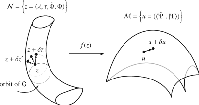
Figure 1: Illustration of the parameter manifold $\mathcal{N}$ and the CC wavefunction manifold $\mathcal{M}$. An element $u\in\mathcal{M}$ is given as the image $u=f(z)$, albeit in a non-unique way. The pre-image $f^{-1}(x)$ is the orbit of a Lie group $\mathsf{G}$ acting on some $z$, illustrated as a closed curves on $\mathcal{N}$ passing through $z$. Thus, there is a manifold of displacements $\delta z$ giving rise to the same displacement $\delta u$. Specifying a gauge selects a unique $\delta z$ (a unique $G$) for each $\delta u$.

The group $\mathsf{G}$ describing mixing of occupied and virtual orbitals separately consists of all block diagonal and invertible matrices on the form

$$G=\begin{pmatrix}[G_{ij}]&0\\ 0&[G_{ab}]\end{pmatrix},$$

i.e, the matrix elements $G_{ia}=G_{ai}=0$. The action on $z$ is defined as follows: The orbitals are transformed according to

$$\Phi\longrightarrow\Phi G,\quad\tilde{\Phi}\longrightarrow G^{-1}\tilde{\Phi},$$ (22)

which preserves biorthogonality. Equation (22) is equivalent to the transformation

$$c^{\dagger}_{p}\longrightarrow\sum_{q}c^{\dagger}_{q}G_{qp},\quad\tilde{c}_{p}\longrightarrow\sum_{q}G^{-1}_{pq}\tilde{c}_{q}.$$

This gives the following transformation on $X_{a}^{i}$:

$$X_{a}^{i}\longrightarrow\sum_{bj}G^{-1}_{ij}X_{b}^{j}G_{ba}.$$

We define the transformation of the amplitudes by

$$\tau_{i}^{a} \longrightarrow\sum_{i^{\prime}a^{\prime}}G_{ii^{\prime}}\tau_{i^{\prime}}^{a^{\prime}}G^{-1}_{a^{\prime}a}$$ (23a)

$$\tau_{ij}^{ab} \longrightarrow\sum_{i^{\prime}j^{\prime}a^{\prime}b^{\prime}}G_{ii^{\prime}}G_{jj^{\prime}}\tau_{i^{\prime}j^{\prime}}^{a^{\prime}b^{\prime}}G^{-1}_{a^{\prime}a}G^{-1}_{b^{\prime}b}$$ (23b)

$$\lambda_{a}^{i} \longrightarrow\sum_{i^{\prime}a^{\prime}}G_{aa^{\prime}}\lambda_{a^{\prime}}^{i^{\prime}}G^{-1}_{i^{\prime}i}$$ (23c)

$$\lambda_{ab}^{ij} \longrightarrow\sum_{i^{\prime}j^{\prime}a^{\prime}b^{\prime}}G_{aa^{\prime}}G_{bb^{\prime}}\tau_{a^{\prime}b^{\prime}}^{i^{\prime}j^{\prime}}G^{-1}_{i^{\prime}i}G^{-1}_{j^{\prime}j}$$ (23d)

with corresponding expressions for higher order excitations. This completes the definition of the action $G\circ z$.

As a consequence of the transformation, $T\longrightarrow T$, $\Lambda\longrightarrow\Lambda$, while $|\phi\rangle\longrightarrow g|\phi\rangle$ and $\langle\tilde{\phi}|\longrightarrow\langle\tilde{\phi}|g^{-1}$, where $g=\det(G_{ij})$. Clearly, $E[z]=E[G\circ z]$. As for the time-dependent functional $S[z(\cdot)]$ it remains to check the part containing the time-derivative, i.e.,

$$\int_{0}^{T}\langle\tilde{\Psi}|\frac{\partial}{\partial t}|\Psi\rangle\;\mathrm{d}t\longrightarrow\int_{0}^{T}\langle\tilde{\Psi}|g^{-1}\frac{\partial}{\partial t}g|\Psi\rangle\;\mathrm{d}t=\int_{0}^{T}\langle\tilde{\Psi}|\frac{\partial}{\partial t}|\Psi\rangle+\frac{\partial\ln g}{\partial t}\;\mathrm{d}t,$$

so the integrand gains only a total time derivative,

$$S[z(\cdot)]\longrightarrow S[G(\cdot)\circ z(\cdot)]=S[z(\cdot)]+\mathrm{i}\hbar\ln[g(T)/g(0)].$$

The last term is a constant with respect to variations vanishing at the end points of $0\leq t\leq T$.

We now proceed to choose a gauge for the orbital rotation group. Suppose we have a solution candidate $z_{0}(t)$, i.e., $\delta S[z_{0}(\cdot)]=0$ for any variation of $z_{0}(t)$. For any choice $G(t)\in\mathsf{G}$, $z(t)=G(t)\circ z_{0}(t)$ is also a solution. To fix a unique solution $z(t)$, we need to find a differential equation for $G(t)$ in terms of $z_{0}(t)$ with a unique solution. To this end, consider the action of $G(t)$ on the orbitals, i.e., $\Phi(t)=\Phi_{0}(t)G(t)$ and $\tilde{\Phi}(t)=G(t)^{-1}\tilde{\Phi}_{0}(t)$. Writing $\eta_{0}(t)=\tilde{\Phi}_{0}(t)\dot{\Phi}_{0}(t)$ and $\eta(t)=\tilde{\Phi}(t)\dot{\Phi}(t)$, we have

$$G(t)\eta(t)=\eta_{0}(t)G(t)+\dot{G}(t).$$

We are free to choose the matrix elements $\dot{G}(t)_{ij}$ and $\dot{G}(t)_{ab}$ of the nonzero blocks $G(t)_{\text{occ}}$ and $G(t)_{\text{vir}}$, respectively, of $G(t)$ at will. Let $g(t)_{ij}$ and $g(t)_{ab}$ be the matrix elements of some arbitrary matrices $g(t)_{\text{occ}}$ and $g(t)_{\text{vir}}$, respectively, and require

$$\dot{G}(t)_{\text{occ}} =G(t)_{\text{occ}}g(t)_{\text{occ}}-\eta_{0}(t)_{\text{occ}}G(t)_{\text{occ}}$$

$$\dot{G}(t)_{\text{vir}} =G(t)_{\text{vir}}g(t)_{\text{vir}}-\eta_{0}(t)_{\text{vir}}G(t)_{\text{vir}}$$

which defines $G(t)$ uniquely. Then,

$$\eta(t)_{\text{occ}}=g(t)_{\text{occ}},\quad\text{and}\quad\eta(t)_{\text{vir}}=g(t)_{\text{vir}}$$

so that any choice of $g(t)_{\text{occ}}$ and $g(t)_{\text{vir}}$, i.e., choice of gauge, implies a specific choice of transformation $G(t)$, and hence a solution representant $z(t)$, all being equivalent [35].

The simplest choice is probably $g(t)_{\text{occ}}\equiv 0$ and $g(t)_{\text{vir}}\equiv 0$, such that

$$\eta(t)=\tilde{\Phi}(t)\dot{\Phi}(t)=\begin{bmatrix}0&[\eta_{ia}]\\ [\eta_{ai}]&0\end{bmatrix}.$$

To derive the differential equations corresponding to this gauge, one needs to perform all possible variations $\delta z(t)$ adhering to the constraint $(\tilde{\Phi}\delta\Phi)_{\text{occ/vir}}=0$, i.e., $\langle\tilde{\varphi}_{i}|\delta{\varphi}_{j}\rangle=\langle\tilde{\varphi}_{a}|\delta{\varphi}_{b}\rangle=0$.

Note that $G(t)$ is simply a theoretical device that describes the continuum of solutions $z(t)$. Using this device we derived conditions on $\dot{z}(t)$ and the variations $\delta z(t)$ that picks exactly one of these solutions. $G(t)$ will not actually be solved for, since it has no physical value.

However, $\mathsf{G}$ as defined above is not the largest group leaving the functionals invariant. It turns out that the singles amplitudes $\tau_{i}^{a}$ may be completely eliminated as well, corresponding to orbital transformations on the form

$$G=e^{\begin{pmatrix}0&0\\ \tau_{i}^{a}&0\end{pmatrix}}.$$

To see this, note that

$$|\Psi\rangle=e^{T}|\phi\rangle=e^{T-T_{1}}e^{T_{1}}|\phi\rangle=e^{T-T_{1}}\left(e^{T_{1}}c^{\dagger}_{1}e^{-T_{1}}\right)\cdots\left(e^{T_{1}}c^{\dagger}_{N}e^{-T_{1}}\right)|-\rangle,$$

and that the transformation $c^{\dagger}_{p}\longrightarrow\exp(T_{1})c^{\dagger}_{p}\exp(-T_{1})$ is equivalent to (see C)

$$\Phi\longrightarrow\Phi e^{\begin{pmatrix}0&0\\ \tau_{i}^{a}&0\end{pmatrix}},\quad\tilde{\Phi}\longrightarrow e^{-\begin{pmatrix}0&0\\ \tau_{i}^{a}&0\end{pmatrix}}\tilde{\Phi}.$$

The dual state $\langle\tilde{\Psi}|$ is invariant:

$$\langle\tilde{\Psi}|=\langle\tilde{\phi}|(1+\Lambda)e^{-T}\longrightarrow\langle\tilde{\phi}|(1+e^{T_{1}}\Lambda e^{-T_{1}})e^{-T+T_{1}}=\langle\tilde{\Psi}|,$$

where we have used that $\langle\tilde{\phi}|e^{T_{1}}=\langle\tilde{\phi}|$. The bivariational functionals are then invariant under the described transformation, and we may set $\tau_{i}^{a}\equiv 0$.

Observe, that we did not transform the amplitudes $\lambda_{a}^{i}$. It is tempting to assume that a transformation on the form

$$G=e^{\begin{pmatrix}0&\sigma_{a}^{i}\\ 0&0\end{pmatrix}}$$

may achieve an elimination of $\lambda_{a}^{i}$. This is not the case. There is no transformation

$$T=\sum_{\mu}\tau^{\mu}X_{\mu}\longrightarrow T^{\prime}=\sum_{\mu}(\tau^{\prime})^{\mu}X_{\mu}$$

with the same truncation level that compensates for the transformation

$$|\Psi\rangle=e^{T}|\phi\rangle\longrightarrow e^{S_{1}}e^{T^{\prime}}e^{-S_{1}}e^{S_{1}}|\phi\rangle=e^{S_{1}}e^{T^{\prime}}|\phi\rangle,$$

i.e., $G$ induces higher-order excitations in $T$. The bivariational functionals therefore cannot be made invariant under the transformation, so $\lambda_{a}^{i}$ cannot be eliminated in this way.

However, it is easy to see, that if we do include $\lambda_{a}^{i}$ as parameters the equations of motion will be overdetermined. The presence of $T_{1}$ is compensated by the freely varying orbitals, but the same is not true for $\Lambda_{1}$. We conclude that in the orbital-adaptive CC, the dual state $\langle\tilde{\Psi}|$ would have more parameters than $|\Psi\rangle$. Correspondingly, $\langle\tilde{\Psi}|$ and $|\Psi\rangle$ would not be one-to-one.

From now on, we therefore set both $\tau_{i}^{a}$ and $\lambda_{a}^{i}$ identically equal to zero, in effect starting with a coupled-cluster doubles, triples, etc, model with adaptive orbitals.

IV.2 Derivation of equations of motion

Performing the variations with respect to the amplitudes is straightforward (see C), and leads to the equations

$$\mathrm{i}\hbar\dot{\tau}^{\mu} =\frac{\partial}{\partial\lambda_{\mu}}\mathcal{E}_{H-\mathrm{i}\hbar D_{0}}[\lambda,\tau,\tilde{\Phi},\Phi]=\langle\tilde{\phi}_{\mu}|e^{-T}(H-\mathrm{i}\hbar D_{0})e^{T}|\phi\rangle$$ (24a)

$$-\mathrm{i}\hbar\dot{\lambda}_{\mu} =\frac{\partial}{\partial\tau^{\mu}}\mathcal{E}_{H-\mathrm{i}\hbar D_{0}}[\lambda,\tau,\tilde{\Phi},\Phi]=\langle\phi|(1+\Lambda)e^{-T}[H-\mathrm{i}\hbar D_{0},X_{\mu}]e^{T}|\phi\rangle$$ (24b)

which must hold for all $\mu\in\mathcal{I}$ included in the approximation. Equations (24) are identical to Equations (20) except for the presence of $D_{0}$ due to the changing orbitals.

Performing the variations with respect to the orbitals, we observe that an arbitrary variation of the one-body function $|\varphi_{p}\rangle=|\varphi_{p}(t)\rangle$ (where we use ket notation for clarity) can be written

$$\delta|\varphi_{p}\rangle=P\delta|\varphi_{p}\rangle+Q\delta|\varphi_{p}\rangle,$$

with $P=\Phi\tilde{\Phi}=\sum_{q}|\varphi_{q}\rangle\langle\tilde{\varphi}_{q}|$ and $Q=1-P$. Due to the gauge choice $\eta^{i}_{j}=\eta^{a}_{b}=0$, we have for the occupied and virtual orbitals

$$\delta|\varphi_{i}\rangle =\sum_{b}\epsilon^{b}_{i}|\varphi_{b}\rangle+Q\delta|\varphi_{i}\rangle$$

and

$$\delta|\varphi_{a}\rangle =\sum_{j}\epsilon^{a}_{j}|\varphi_{j}\rangle+Q\delta|\varphi_{a}\rangle,$$

respectively, where $\epsilon^{a}_{i}$ are arbitrary independent functions of time, and $Q\delta|\varphi_{i}\rangle$ is completely arbitrary and independent from the $\epsilon^{a}_{i}$. We may therefore perform the variations in two stages: First, we set $\delta|\varphi_{i}\rangle=\epsilon(t)|\varphi_{a}\rangle$ for each $a,i$ separately (then exchange $i$ and $a$), and then finally we set $\delta|\varphi_{p}\rangle=|\theta\rangle=Q|\theta\rangle$.

Beginning with the $P$-part of the variations, we note that the variations in $\langle\tilde{\varphi}_{p}|$ are linked to those of $|\varphi_{p}\rangle$ due to the biorthogonality constraint. We get

$$0=\delta\langle\tilde{\varphi}_{a}|\varphi_{i}\rangle=\langle\delta\tilde{\varphi}_{a}|\varphi_{i}\rangle+\epsilon(t)\quad\Leftrightarrow\quad\delta\langle\tilde{\varphi}_{a}|=-\epsilon(t)\langle\tilde{\varphi}_{i}|.$$

It is useful to consider an arbitrary $|u\rangle$ and $\langle v|$, whose variations are

$$\delta|u\rangle=\epsilon c^{\dagger}_{a}\tilde{c}_{i}|u\rangle\quad\text{and}\quad\delta\langle v|=-\epsilon\langle v|c^{\dagger}_{a}\tilde{c}_{i},$$

so that we have the general equation

$$\delta\langle u|A|v\rangle=\epsilon\langle u|[A,c^{\dagger}_{a}\tilde{c}_{i}]|v\rangle+\langle u|(\delta A)|v\rangle,$$

where $A$ is any operator that may depend explicitly on the orbitals. (If $A$ does not depend on the orbitals, then $\delta A=0$.) For example, the Hamiltonian does not depend explicitly on the orbitals, while

$$\delta D_{0}=\delta\sum_{q}\dot{c}^{\dagger}_{q}\tilde{c}_{q}=\left(\dot{\epsilon}c^{\dagger}_{a}+\epsilon\dot{c}^{\dagger}_{a}\right)\tilde{c}_{i}-\epsilon\dot{c}^{\dagger}_{a}\tilde{c}_{i}=\dot{\epsilon}c^{\dagger}_{a}\tilde{c}_{i}.$$

We also note that

$$\delta\sum_{\mu}\dot{\tau}^{\mu}\langle\tilde{\Psi}|X_{\mu}|\Psi\rangle=0,$$

since the expectation value of $X_{\mu}$ only depends on the amplitudes and not the orbitals. We compute the variation in $\mathcal{S}$:

$$\delta\mathcal{S} =\delta\int_{0}^{T}\langle\tilde{\Psi}|\mathrm{i}\hbar D_{0}+\mathrm{i}\hbar\sum_{\mu}\dot{\tau}^{\mu}X_{\mu}-H|\Psi\rangle\;\mathrm{d}t$$

$$=\int_{0}^{T}\epsilon(t)\langle\tilde{\Psi}|[\mathrm{i}\hbar D_{0}-H,c^{\dagger}_{a}\tilde{c}_{i}]|\Psi\rangle+\mathrm{i}\hbar\dot{\epsilon}(t)\langle\tilde{\Psi}|c^{\dagger}_{a}\tilde{c}_{i}|\Psi\rangle\;\mathrm{d}t$$ (25)

$$=\int_{0}^{T}\epsilon(t)\left(\langle\tilde{\Psi}|[\mathrm{i}\hbar D_{0}-H,c^{\dagger}_{a}\tilde{c}_{i}]|\Psi\rangle-\mathrm{i}\hbar\dot{\rho}^{i}_{a}\right)\;\mathrm{d}t.$$

Requiring $\delta\mathcal{S}=0$ for all $\epsilon(t)$ implies that the integrand must vanish. Using the gauge condition, $D_{0}$ becomes

$$D_{0}=\sum_{jb}\eta^{j}_{b}c^{\dagger}_{j}\tilde{c}_{b}+\sum_{jb}\eta^{b}_{j}c^{\dagger}_{b}\tilde{c}_{j},$$

and only the first sum survives in the commutator in Eqn. (25). We obtain the equation

$$\mathrm{i}\hbar\sum_{bj}\langle\tilde{\Psi}|[c^{\dagger}_{j}\tilde{c}_{b},c^{\dagger}_{a}\tilde{c}_{i}]|\Psi\rangle\eta^{b}_{j}=\mathrm{i}\dot{\rho}^{i}_{a}+\langle\tilde{\Psi}|[H,c^{\dagger}_{a}\tilde{c}_{i}]|\Psi\rangle,$$ (26)

which is a linear equation for $\eta^{b}_{j}=\langle\tilde{\varphi}_{b}|\dot{\varphi}_{j}\rangle$. It is readily verified that

$$\rho^{i}_{a}=\langle\tilde{\Psi}|c^{\dagger}_{a}\tilde{c}_{i}|\Psi\rangle=\langle\tilde{\phi}|(1+\Lambda)e^{-T}X_{i}^{a}e^{T}|\phi\rangle=\lambda_{a}^{i}\equiv 0,$$

and that

$$[c^{\dagger}_{p}\tilde{c}_{q},c^{\dagger}_{a}\tilde{c}_{i}] =\delta^{q}_{a}c^{\dagger}_{p}\tilde{c}_{i}-\delta^{i}_{p}c^{\dagger}_{a}\tilde{c}_{q}$$ (27a)

$$[c^{\dagger}_{p}c^{\dagger}_{r}\tilde{c}_{s}\tilde{c}_{q},c^{\dagger}_{a}\tilde{c}_{i}] =\delta^{q}_{a}c^{\dagger}_{p}c^{\dagger}_{r}\tilde{c}_{s}\tilde{c}_{i}-\delta^{s}_{a}c^{\dagger}_{p}c^{\dagger}_{r}\tilde{c}_{q}\tilde{c}_{i}+\delta^{i}_{r}c^{\dagger}_{a}c^{\dagger}_{p}\tilde{c}_{s}\tilde{c}_{q}-\delta^{i}_{p}c^{\dagger}_{a}c^{\dagger}_{r}\tilde{c}_{s}\tilde{c}_{q}.$$ (27b)

The coefficient matrix of Eqn. (26) becomes

$$A^{ib}_{aj}\equiv\langle\tilde{\Psi}|[c^{\dagger}_{j}\tilde{c}_{b},c^{\dagger}_{a}\tilde{c}_{i}]|\Psi\rangle=\delta^{b}_{a}\rho^{i}_{j}-\delta^{i}_{j}\rho^{b}_{a}.$$ (28)

In total, we get a linear equation for $\eta^{b}_{j}$ that reads

$$\mathrm{i}\hbar\sum_{bj}A^{ib}_{aj}\eta^{b}_{j}=\sum_{p}\rho^{i}_{p}h^{p}_{a}-\sum_{q}\rho^{q}_{a}h^{i}_{q}+\frac{1}{2}\left[\sum_{prs}\rho^{is}_{pr}u^{pr}_{as}-\sum_{rqs}\rho^{qs}_{ar}u^{ir}_{qs}\right],$$

where we used Eqns. (27) and the anti-symmetry $u^{pr}_{qs}=-u^{pr}_{sq}$.

We now turn to the variation $\delta|\varphi_{a}\rangle=\epsilon(t)|\varphi_{i}\rangle$, which implies $\delta\langle\tilde{\varphi}_{i}|=-\epsilon(t)\langle\tilde{\varphi}_{a}|$. The calculation is completely analogous to the previous case, so we simply state the result,

$$-\mathrm{i}\hbar\sum_{bj}A^{ja}_{bi}\eta^{j}_{b}=\sum_{p}\rho^{a}_{p}h^{p}_{i}-\sum_{q}\rho^{q}_{i}h^{a}_{q}+\frac{1}{2}\left[\sum_{prs}\rho^{as}_{pr}u^{pr}_{is}-\sum_{rqs}\rho^{qs}_{ir}u^{ar}_{qs}\right]+\mathrm{i}\hbar\dot{\rho}^{a}_{i}.$$

Unlike $\rho_{a}^{i}$, the coefficients $\rho^{a}_{i}$ do not vanish identically, except for in the doubles only approximation to be considered in Section IV.3.

Having derived the equations of motion for the $P$-part of $\dot{\varphi}_{p}$ (and therefore also $\dot{\tilde{\varphi}}_{p}$), we now turn to the $Q$-part. We perform an arbitrary variation $\delta\langle\tilde{\varphi}_{p^{\prime}}|\equiv\langle\theta|=\langle\theta|Q$, i.e., $\langle\theta|\varphi_{q}\rangle=0$ for all $q$. These variations are therefore independent from the corresponding variations in $|\varphi_{q}\rangle$.

It is convenient to use $\mathcal{S}$ on the form (18b) to derive the variational equations. Recall that the reduced density matrix elements $\rho^{q}_{p}$ and $\rho^{qs}_{pr}$ are independent of the orbitals, since they are computed only using the anti-commutator (9). Thus, the only quantities that vary are the one- and two-body matrix elements $h^{p}_{q}$, $\eta^{p}_{q}$ and $u_{qs}^{pr}$:

$$\delta\mathcal{S} =\delta\int_{0}^{T}\sum_{pq}\rho^{q}_{p}(\mathrm{i}\hbar\eta^{p}_{q}-h^{p}_{q})-\frac{1}{4}\sum_{prqs}\rho^{qs}_{pr}u^{pr}_{qs}\;\mathrm{d}t$$

$$=\int_{0}^{T}\sum_{q}\rho^{q}_{p^{\prime}}\langle\theta|(\mathrm{i}\hbar\frac{\partial}{\partial t}-h)|\varphi_{q}\rangle-\frac{4}{4}\sum_{qrs}\rho^{qs}_{p^{\prime}r}\langle\theta\tilde{\varphi}_{r}|u|\varphi_{q}\varphi_{s}\rangle\;\mathrm{d}t$$ (29)

$$=\int_{0}^{T}\langle\theta|\left[\sum_{q}\rho^{q}_{p^{\prime}}(\mathrm{i}\hbar|\dot{\varphi_{q}}\rangle-h|\varphi_{q}\rangle)-\sum_{qrs}\rho^{qs}_{p^{\prime}r}\langle\;\cdot\;\tilde{\varphi}_{r}|u|\varphi_{q}\varphi_{s}\rangle\right]\;\mathrm{d}t$$

From line 1 to line 2 we used the symmetries $u^{pr}_{qs}=u^{rp}_{sq}$ and $\rho^{qs}_{pr}=\rho^{sq}_{rp}$, and the two-electron integrals in the last two lines are not anti-symmetrized. We define mean-field potentials $W^{r}_{s}$ by

$$\langle\;\cdot\;\tilde{\varphi}_{r}|u|\varphi_{q}\varphi_{s}\rangle\equiv\int\tilde{\varphi}_{r}(x^{\prime})u(x,x^{\prime})\varphi_{q}(x)\varphi_{s}(x^{\prime})\;\mathrm{d}x\equiv W^{r}_{s}|\varphi_{q}\rangle.$$

Since Eqn. (29) must hold for all $\langle\theta|=\langle\theta|Q$, we get the equation

$$\mathrm{i}\hbar\sum_{q}\rho^{q}_{p}Q\frac{\partial}{\partial t}|\varphi_{q}\rangle=\sum_{q}\rho^{q}_{p}Qh|\varphi_{q}\rangle+\sum_{qrs}\rho^{qs}_{pr}QW^{r}_{s}|\varphi_{q}\rangle\quad\text{for all $p$}.$$

Performing the variation $\delta|\varphi_{q}\rangle=|\theta\rangle=Q|\theta\rangle$ is completely analogous, and gives

$$-\mathrm{i}\hbar\sum_{p}\rho^{q}_{p}\left(\frac{\partial}{\partial t}\langle\tilde{\varphi}_{p}|\right)Q=\sum_{p}\rho^{q}_{p}|\tilde{\varphi}_{p}\rangle hQ+\sum_{prs}\rho^{qs}_{pr}\langle\tilde{\varphi}_{p}|W^{r}_{s}Q\quad\text{for all $q$},$$

where the minus sign comes from integration by parts.

IV.3 The doubles approximation: OATDCCD

The simplest non-trivial OATDCC case is the doubles approximation (OATDCCD). The wavefunction parameters are, in addition to the orbitals $\tilde{\Phi}$ and $\Phi$, the amplitudes $\tau=(\tau_{ij}^{ab})$ and $\lambda=(\lambda_{ab}^{ij})$. In A, a complete listing of the algebraic expressions needed to evaluate the equations of motion is given. In particular, the only nonzero elements of the one-body reduced density matrix are $\rho^{j}_{i}$ and $\rho^{b}_{a}$, which simplifies the equations of motion. The amplitude equations read

$$\mathrm{i}\hbar\dot{\tau}_{ij}^{ab} =\frac{\partial}{\partial\lambda_{ab}^{ij}}\mathcal{E}_{H}[\lambda,\tau,\tilde{\Phi},\Phi]=\langle\tilde{\phi}_{ij}^{ab}|e^{-T}He^{T}|\phi\rangle$$ (30a)

$$-\mathrm{i}\hbar\dot{\lambda}_{ab}^{ij} =\frac{\partial}{\partial\tau^{ab}_{ij}}\mathcal{E}_{H}[\lambda,\tau,\tilde{\Phi},\Phi]=\langle\tilde{\phi}|(1+\Lambda)e^{-T}[H,X^{ij}_{ab}]e^{T}|\phi\rangle.$$ (30b)

The $$P$$-space orbital equations read

$$\mathrm{i}\hbar\sum_{bj}A^{ib}_{aj}\eta^{b}_{j} =\sum_{j}\rho^{i}_{j}h^{j}_{a}-\sum_{b}\rho^{b}_{a}h^{i}_{b}+\frac{1}{2}\left[\sum_{prs}\rho^{is}_{pr}u^{pr}_{as}-\sum_{rqs}\rho^{qs}_{ar}u^{ir}_{qs}\right]$$ (30c)

$$-\mathrm{i}\hbar\sum_{bj}A^{ja}_{bi}\eta^{j}_{b} =\sum_{b}\rho^{a}_{b}h^{b}_{i}-\sum_{j}\rho^{j}_{i}h^{a}_{j}+\frac{1}{2}\left[\sum_{prs}\rho^{as}_{pr}u^{pr}_{is}-\sum_{rqs}\rho^{qs}_{ir}u^{ar}_{qs}\right].$$ (30d)

Finally, the $$Q$$-space orbital equations are

$$\mathrm{i}\hbar\sum_{q}\rho^{q}_{p}Q\frac{\partial}{\partial t}|\varphi_{q}\rangle =\sum_{q}\rho^{q}_{p}Qh|\varphi_{q}\rangle+\sum_{qrs}\rho^{qs}_{pr}QW^{r}_{s}|\varphi_{q}\rangle\quad$$ (30e)

$$-\mathrm{i}\hbar\sum_{p}\rho^{q}_{p}\left(\frac{\partial}{\partial t}\langle\tilde{\varphi}_{p}|\right)Q =\sum_{p}\rho^{q}_{p}|\tilde{\varphi}_{p}\rangle hQ+\sum_{prs}\rho^{qs}_{pr}\langle\tilde{\varphi}_{p}|W^{r}_{s}Q.$$ (30f)

The coefficients $A^{ib}_{aj}$ are defined in Eqn. (28). The right-hand sides of Equations (30a) and (30b), which are polynomials in terms of $\tau_{ij}^{ab}$, $\lambda_{ab}^{ij}$, $h^{p}_{q}$ and $u^{pr}_{qs}$, can be found in the Appendix. Note that the right-hand sides of the equations are identical to the one used in standard CCD calculations for the ground state energy, since the operator $D_{0}$ is eliminated due to $\rho^{a}_{i}=\rho^{i}_{a}=0$. Existing computer codes may be helpful for implementations.

Since $D_{0}$ drops from (30a) and (30b), the right hand sides can be evaluated independently of Eqns. (30c) to (30f). Note that to evaluate $\dot{\tilde{\Phi}}$ and $\dot{\Phi}$, $\eta$ must be solved for in addition to $Q|\dot{\varphi}_{q}\rangle$ and $\langle\dot{\tilde{\varphi}}_{p}|Q$. The results are assembled according to

$$|\dot{\varphi}_{q}\rangle =(P+Q)|\dot{\varphi}_{q}\rangle=\sum_{p}|\varphi_{p}\rangle\langle\tilde{\varphi}_{p}|\dot{\varphi}_{q}\rangle+Q|\dot{\varphi}_{q}\rangle=\sum_{p}\eta^{p}_{q}|\varphi_{p}\rangle+Q|\dot{\varphi}_{q}\rangle$$

$$\langle\dot{\tilde{\varphi}}_{p}| =\langle\dot{\tilde{\varphi}}_{p}|(P+Q)=\sum_{q}\langle\dot{\tilde{\varphi}}_{p}|\varphi_{q}\rangle\langle\tilde{\varphi}_{q}|+\langle\dot{\tilde{\varphi}}_{q}|Q=-\sum_{q}\eta^{p}_{q}\langle\tilde{\varphi}_{q}|+\langle\dot{\tilde{\varphi}}_{p}|Q$$

We note that the $Q$-space equation for $|\varphi_{p}\rangle$ is formally identical to the orbital equation of MCTDHF (see B), and the equation for $\langle\dot{\tilde{\varphi}}_{p}|$ is formally identical to the complex conjugate. However, in the CC case the matrices $u_{pr}^{qs}$, $h^{p}_{q}$ and $\rho^{q}_{p}$ are not exactly Hermitian. Therefore, the two equations are only complex conjugates of each other to within an approximation, and both must be propagated.

We will now consider the computational cost of evaluating the time derivatives in a computer implementation. We will in the following assume a grid-based discretization of single-particle space using in total $N_{b}$ points. In particular, integrals are evaluated as sums with $N_{b}$ elements.

We consider first the computation of the amplitude equations (30a) and (30b), assuming that $h^{p}_{q}$ etc are available in computer memory. It is easy to see, from Equations (42) and (47), that by brute-force summation the worst-scaling terms require $O(N^{4}(L-N)^{4})=O(L^{8})$ operations for computing the totality of derivatives, which is a conservative estimate since $N<L$. Existing CC codes typically reduce this to $O(L^{6})$ by clever use of intermediate variables [15].

The $P$-space orbital equations (30c) and (30d) are linear equations where a vector of dimension $O(L^{2})$ is to be solved for. This requires at most $O(L^{6})$ operations. The right-hand side is dominated by the two-body terms, which cost $O(L^{5})$ in total to compute.

We next turn to the $Q$-space orbital equations (30e) and (30f), which can be viewed as differential equations for matrices of dimension $N_{b}\times L$ and $L\times N_{b}$, respectively. The cost analysis is identical for the two. The matrix $\rho^{q}_{p}$ needs to be inverted, a step of at most $O(L^{3})$ cost. Multiplying Eqn. (30e) by the inverse matrix elements of $\rho^{q}_{p}$ shows that the $Q$-part of $\mathrm{i}\hbar|\dot{\varphi}_{p}\rangle$ can be computed as the sum of $Qh|\varphi_{p}\rangle$ and a two-body mean-field term which clearly dominates the computation. The cost of this term is $O(L^{3}N_{b})$ plus $O(L^{2}N_{b})$ for the multiplication of the result with $\rho^{-1}$.

Unlike standard CC calculations, the one- and two-electron integrals $h^{p}_{q}$ and $u^{pr}_{qs}$ must be updated at each time $t$. This is similar to the situation in MCTDHF theory. Moreover, equations (30c)–(30f) are formulated in terms of the reduced one- and two-electron matrices which need to be computed.

The matrices $\rho^{q}_{p}$ and $\rho^{qr}_{ps}$ cost less than the evaluation of the orbital equations right-hand sides in total, and $h^{p}_{q}$ is relatively cheap to compute. However, the two-electron integrals and the mean-field functions $W^{r}_{s}$ are costly. The computation of all the mean-fields, which are local functions, costs $O(L^{2}N_{b}^{2})$. Since $u^{pq}_{qs}=\langle\tilde{\varphi}_{p}|W^{r}_{s}|\varphi_{q}\rangle$, the computation of the two-electron integrals costs an additional $O(L^{4}N_{b})$ operations.

The computation of $W^{r}_{s}$ is in fact very expensive, being similar in cost to computing two-particle integrals, i.e., six-dimensional integrals in realistic calculations. This problem is ubiquitous for all time-dependent mean-field calculations, and a common approach is to employ some low-rank expansion for the interaction potential $u(x,x^{\prime})$, which needs to be sampled at the grid points $\xi_{k}$, $k=1,\cdots,N_{b}$. The resulting matrix $v(\xi_{k},\xi_{k^{\prime}})$ is symmetric, with eigenvalue decomposition

$$v(\xi_{k},\xi_{k^{\prime}})=\sum_{m=1}^{N_{b}}\lambda_{m}f_{m}(\xi_{k})f_{m}(\xi_{k^{\prime}}),$$ (31)

where $f_{m}$ is the eigenvector belonging to $\lambda_{m}$, the latter arranged in decreasing order. The optimal (in the 2-norm) $M$-term approximation to $v(\xi_{k},\xi_{k^{\prime}})$ is then obtained by truncating Eqn. (31) after $M$ terms. Oftentimes, only a small number $M\ll N_{b}$ terms are needed. Moreover, if $N_{b}$ is increased, $M$ may typically be held fixed. The mean-fields then become

$$W^{r}_{s}(\xi_{k})\approx\sum_{m=1}^{M}\lambda_{m}v_{m}(\xi_{k})\langle\tilde{\varphi}_{r}|v_{m}|\varphi_{s}\rangle,$$

which reduces the cost of computing $W_{s}^{r}$ to $O(N_{b}L^{2})$ for the inner products plus $O(L^{2}N_{b}M)$ for the summation, reducing the cost proportionally to the fraction $M/N_{b}$ of modes included in Eqn. (31).

To sum up, we see that the cost of evaluating the right-hand sides of the equations of motion is dominated by the computation of the $W^{r}_{s}$ and $u^{qr}_{ps}$ and of the evaluation of the amplitude equations, costing $O(N^{4}(L-N)^{4})$ (if no optimization is done), and being the only terms that increase in complexity with the number $N$ of particles. This should be contrasted to MCTDHF calculations, where the number of amplitudes grow exponentially with $N$.

V Further properties of OATDCC

V.1 Relations to other methods

It is instructive to consider special cases of the OATDCC method and relate these to other, well-known wavefunction approximations.

In the case where all excitation levels are included, we have seen that the CC ansatz becomes the FCI ansatz within the chosen basis. Therefore, the MCTDHF and OATDCC methods are equivalent in this limit. In B an explicit derivation of MCTDHF using the bivariational principle is carried out. Note, however, that the gauge conditions are different, i.e., the orbitals produced are not identical. This stems from the fact that the CC wavefunction is normalized according to $\langle\tilde{\phi}|\Psi\rangle=1$ at all times. However, the orbitals in the two methods span the same space, and the wavefunctions are identical except for normalization. At each time $t$, the OATDCC and MCTDHF wavefunctions produce the same expectation value functional for any observable.

At the other end of the hierarchy, we find the trivial case where there are no amplitudes at all, i.e., we take $L=N$ and $\Lambda=T=0$. In that case, the OATDCC energy expectation functional becomes

$$\mathcal{E}_{H}[\Phi,\tilde{\Phi}] =\langle\tilde{\phi}|H|\phi\rangle=\langle\tilde{\phi}|\left(\sum_{pq}h^{p}_{q}c^{\dagger}_{p}\tilde{c}_{q}+\frac{1}{4}\sum_{pqrs}u^{pr}_{qs}c^{\dagger}_{p}c^{\dagger}_{r}\tilde{c}_{s}\tilde{c}_{q}\right)|\phi\rangle$$

$$=\sum_{p}\langle\tilde{\varphi}_{p}|h|\varphi_{p}\rangle+\frac{1}{2}\sum_{pr}\langle\tilde{\varphi}_{p}\tilde{\varphi}_{r}|u|\varphi_{p}\varphi_{r}\rangle_{AS}.$$

This is the Hartree–Fock energy functional (when $\tilde{\Phi}=\Phi^{\mathsf{H}}$). Thus, the conditions for $\delta\mathcal{E}_{H}=0$ are the Hartree–Fock equation and its complex conjugate. The action functional becomes

$$\mathcal{S}[\Phi,\tilde{\Phi}] =\int_{0}^{T}\langle\tilde{\phi}|(\mathrm{i}\hbar D_{0}-H)|\phi\rangle\;\mathrm{d}t$$

$$=\int_{0}^{T}\mathrm{i}\hbar\sum_{p}\langle\tilde{\varphi}_{p}|\dot{\varphi}_{p}\rangle-\sum_{p}\langle\tilde{\varphi}_{p}|h|\varphi_{p}\rangle-\frac{1}{2}\sum_{pr}\langle\tilde{\varphi}_{p}\tilde{\varphi}_{r}|u|\varphi_{p}\varphi_{r}\rangle_{AS}\;\mathrm{d}t.$$

This is the time-dependent Hartree–Fock (TDHF) functional. Computing the variation with respect to $\tilde{\varphi}_{q}$ we get the TDHF equations of motion, and the variation with respect to $\varphi_{q}$ gives the complex conjugate, showing that the $T=\Lambda=0$ case is indeed equivalent to TDHF.

We also note that the OATDCCD approximation is equivalent to MCTDHF whenever $N=2$. Moreover, some combinations of $L$ and $N$ also give equivalence, for example $L=N+2$ since there are no triple excitations defined.

Finally, in the absence of interactions, the Hamiltonian is a pure one-body Hamiltonian. One can easily show that the choice $\mathrm{i}\hbar\dot{\Phi}=H\Phi$, $-\mathrm{i}\hbar\dot{\tilde{\Phi}}=\tilde{\Phi}H$ and $\dot{\lambda}_{\mu}=\dot{\tau}^{\mu}=0$ gives $\mathcal{S}[\lambda,\tau,\tilde{\Phi},\Phi]=0$ and a stationary $\mathcal{S}$. This is the exact solution to the dynamics for any initial condition. (The gauge conditions in this case are chosen differently from earlier: $\eta^{i}_{j}=\langle\tilde{\varphi}_{i}|\dot{\varphi}_{j}\rangle=\langle\tilde{\varphi}_{i}|H^{(1)}|\varphi_{j}\rangle/\mathrm{i}\hbar$ and $\eta^{a}_{b}=\langle\tilde{\varphi}_{a}|H^{(1)}|\varphi_{b}\rangle/\mathrm{i}\hbar$.)

In OATDCC the evolution of the orbitals are chosen to variationally optimize the action functional. As early as 1978, Hoodbhoy and Negele [19] discussed a time-dependent CC approach using an explicit dependence of time in the orthonormal single-particle functions. This would correspond to using the following functional to define the evolution:

$$\mathcal{S}_{\text{H--N}}[\tau,\lambda]=\int_{0}^{T}\mathrm{i}\hbar\lambda_{\mu}\dot{\tau}^{\mu}-\langle\tilde{\phi}|(1+\Lambda)e^{-T}(H-\mathrm{i}\hbar D_{0}(t))e^{T}|\phi\rangle\;\mathrm{d}t.$$

The $D_{0}$ operator simply is a correction in the standard CC Lagrangian due to a moving basis. Hoodbhoy and Negele suggested computing the time-dependence of $\Phi$ using, say, TDHF, i.e., a TDHF calculation is first performed, and the output is fed into $\mathcal{S}_{\text{H--N}}$. However, this approach would have inferior approximation properties compared to OATDCC while at the same time being only marginally easier to evolve in time. To see this, consider the fact that the TDHF solution would depend only on the initial choice of the orbitals, and not on the full state at time $t$ as in the OATDCC approach. The OATDCC orbitals will generally differ substantially from the TDHF solution, since their motion is computed from the wavefunctions at time $t$. The Hoodbhoy–Negele TDHF approach neglects the correlation effects built into the wavefunction during the evolution. As for the computational cost, note that TDHF needs the computation of the two-particle integrals, so one gains very little, if nothing, at simplifying to TDHF for the orbitals.

V.2 Approximation properties

We now ask: what kinds of systems can we expect to be able to treat with OATDCC, and what systems cannot be expected to give good results?

The usual CC ansatz (with fixed orbitals) is based on a single reference determinant, incorporating correlations through the cluster operator. For good results, the reference determinant should be a “large” part of the wavefunction. In the language of computational chemistry, dynamic correlation (which by definition is due to the interparticle interactions) must be dominating, while static correlation (arising from degeneracies in the spectrum) should be small.

For a dynamical calculation we must correspondingly require that, for all $t\geq 0$, the wavefunction is a single-reference type state. This is reasonable whenever the initial condition is of such type: intuitively, the Hamiltonian cannot generate static correlation since the only source of correlation from dynamics is the interparticle interaction. This is actually observed in the numerical experiment in Section VI.

However, standard CC is known to perform adequately even in the presence of static correlation, which gives reason to believe that the same holds true for OATDCC calculations. In any case, OATDCCD should be much better than a singles-and doubles truncation of MCTDHF due to size-consistency, even though the latter is a “true” multiconfigurational method, where all the basis determinants are independent.

It is worthwhile to note, that for systems with spin, the OATDCC ansatz is not an eigenfunction of the total spin; only of the total spin projection along some preselected direction in space $z$. This is, however, not a problem in general if $H$ commutes with total spin: all expectation values for spin-independent observables are the same as for the properly “spin-symmetrized” wavefunction.

V.3 Non-feasibility of imaginary time relaxation

We have not yet discussed choices of initial conditions for OATDCC calculations. Typically, one would like to start in the ground state of the system under consideration, or a state closely related to this. Indeed, the orbital-adaptive CC ansatz could in principle be used for ground-state calculations in the first place, just like MCTDHF actually is a time-dependent version of the multi-configuration Hartree–Fock (MCHF) for computing eigenvalues of $H$.

The ground state is a critical point for $\mathcal{E}_{H}$, and in MCTDHF theory this can be computed using imaginary time propagation, that is to say, formally replacing the time $t$ with $-\mathrm{i}s$; so-called Wick rotation. Asymptotically, as $s\rightarrow\infty$, a critical point of the variational energy is obtained. This is a quite robust procedure for variational approximations. For non-variational methods like coupled-cluster, the situation is, literally, more complex.

To see this, consider again local coordinates $z(t)\in\mathbb{C}^{n}$. The equations of motion for $z(t)$ are analytic in both $z$ and $t$. Thus, the energy is an analytic function of $t$, which is conserved, $\mathrm{d}\mathcal{E}[z(t)]/\mathrm{d}t\equiv 0$. Thus, the energy is a constant analytic function, even for complex $t$. Thus, the energy will not decay exponentially when the system is propagated in imaginary time.

We conclude that computing the ground state using imaginary time propagation is not straightforward and requires separate study. Instead, quasi-Newton schemes like those already used for standard CC could be used, but we will not investigate this further in the present article.

Suppose the ground state is desired as initial condition. One option is to perform a Hartree–Fock calculation to generate a set of orbitals, and then perform a CCD calculation within this basis. This is the standard practice for molecular calculations, and even though not an exact critical point of the OATDCC energy, it should be a suitable starting point for dynamics calculations. In our numerical experiment in Section VI we choose a similar approach.

VI A numerical experiment

VI.1 Outline and model system

A numerical experiment on a model system mimicking electron-atom collision has been performed in order to test the OATDCCD method against the standard MCTDHF method. (Recall that OATDCCD is an approximation to MCTDHF.) Generic MCTDHF and OATDCCD codes has been written from scratch. The MCTDHF code was tested against numerical experiments reported in the literature [7] and found to agree perfectly with these. The OATDCCD code uses the algebraic expressions listed in A for the equations of motion. The code is tested against MCTDHF computations for special combinations of $L$ and $N$ where the two ansätze are equivalent. Perfect agreement was found, indicating the correctness of the implementation.

The numerical experiment consists of two phases: (1) preparation of the initial wavefunction, and (2) propagation of this state from $t=0$ to $t=t_{\text{final}}$ using both MCTDHF and OATDCC while monitoring some observables. In particular the energy $\mathcal{E}_{H}$ should be conserved at all times.

The test system is defined as follows. Consider a model consisting of $N$ electrons in one spatial dimension. The orbitals are functions $\varphi_{p}(x,s)$, where $x\in\mathbb{R}$ is the spatial position and $s\in\{-\frac{1}{2},+\frac{1}{2}\}$ is the quantum number of the projection of the electron spin along some arbitrary axis.

The particles interact via a smoothed Coulomb force (for simplicity) and an external Gaussian well potential. The Hamiltonian of the system has one-body part

$$h=-\frac{1}{2}\frac{\partial^{2}}{\partial x^{2}}+V(x),\quad V(x)=-V_{0}e^{-x^{2}/2a^{2}},$$

where $V_{0}=7$ and $a=1.5$ are the parameters of the Gaussian well. The smoothed Coulomb interaction is given by

$$u(x_{1},x_{2})=\frac{\lambda}{\sqrt{|x_{1}-x_{2}|+\delta^{2}}},$$

and we use parameters $\lambda=1$ and $\delta=0.2$. These are reasonable parameters for, say, a quantum wire model [36].

The complete Hamiltonian is seen to commute with any spin operator. We remark that if (1) the initial orbitals are spin-orbitals on the form $\varphi_{p}(x,s)=\psi_{p}(x)\chi_{\sigma_{p}}(s)$ where $\chi_{\sigma}$ is a spinor basis function, and if (2) the initial wavefunction is an eigenfunction for the total spin projection operator, the equations of motion (30) preserve these properties. That is to say, under these conditions the orbitals are always on product form

$$\varphi_{p}(x,s,t)=\psi_{p}(x,s,t)\chi_{\sigma_{p}}(s),$$

and the wavefunction remains an eigenfunction of the total spin projection.

VI.2 Discretization and propagation scheme

We discretize the one-particle coordinates by introducing a standard discrete Fourier transform-based discretization over the interval $[-R,R]$ using $N_{\text{grid}}=64$ points [37]. The total number of basis functions is then $N_{b}=2N_{\text{grid}}=128$. The kinetic energy operator is evaluated using the fast Fourier transform (FFT) and is highly efficient and accurate. In our calculations, we set $R=15$. The orbital matrices $\tilde{\Phi}$ and $\Phi$ become standard matrices of dimension $L\times N_{b}$ and $N_{b}\times L$, respectively, giving a simple representation in the computer code.

For propagation, we choose a variational splitting scheme [38]. Variational splitting is a generalization of the standard split-step scheme used for brute-force grid discretizations of few-body problems [37]. Using this scheme, the time step $\Delta t$ can be chosen relatively large and independently of the grid spacing $\Delta x$. Variational splitting is most easily described in terms of a time-dependent Hamiltonian $\tilde{H}(t)=T+\sum_{n=-\infty}^{\infty}\delta(t-(n+1/2)\Delta t)(H-T)$, where $T$ is the kinetic energy operator and $H-T$ is the remaining potential terms. A time step then consists of three steps: (1) Propagation using kinetic energy only as a time step $\Delta t/2$, (2) Propagation using $H-T$ only a time step $\Delta t$ using a fourth order Runge–Kutta for simplicity, and finally step (1) is repeated. The key point is that the stability of the scheme becomes insensitive to $\Delta x$, and that step (1) is evaluated exactly without involving the amplitudes at all. The local error is of order $\Delta t^{3}$. A simple integration of Eqns. (30) using, say, Runge–Kutta will require a time step $\Delta t\sim\Delta x^{2}$. In multi-configurational time-dependent Hartree calculations, other ways of eliminating this stability problem than variational splitting is often used, e.g., the constant mean-field scheme [2]. However, this requires more coding effort than variational splitting which is sufficient for our modest purposes.

VI.3 Preparation of initial wavefunction

We need initial wavefunctions for both the MCTDHF and OATDCCD ansätze. The former is computed as follows.

The parameters of the Gaussian well potential and interaction potential are experimentally chosen so that they support an $N=4$ ground state $|\Psi_{4}\rangle$ with total spin projection zero. This ground state is computed in the MCTDHF scheme using imaginary time propagation of the equations of motion from a random initial condition.

In order to generate non-trivial but easily understood dynamics, we prepare a fifth particle in a classical-like Gaussian wavepacket $g(x,s)$ given by

$$g(x,s)=C\exp\left[-(x-x_{0})^{2}/(4\sigma^{2})+\mathrm{i}k_{0}x\right]\chi_{+1/2}(s),$$

where $C$ is a normalization constant, $x_{0}$ the “starting position” of the particle, and $k_{0}$ is the “starting momentum”. The parameter $\sigma$ controls the width of the wavepacket. For our experiment, we choose $x_{0}=10$, $k_{0}=1.2$, and, $\sigma=1.25$. Note that we (arbitrarily) choose spin $+1/2$ for this particle. The initial MCTDHF state is then

$$|\Psi\rangle=g^{\dagger}|\Psi_{4}\rangle,$$

where $g^{\dagger}$ is the creation operator associated with $g(x,s)$. The complete wavefunction therefore intuitively describes an incoming electron on collision course with a bound beryllium-like “atom” in the ground state.

In terms of the MCTDHF parameters, the addition of the particle simply corresponds to extending the orbital matrix $\Phi$ with an extra column (orthogonalized against the others), in addition to a lot of zeroes in the MCTDHF coefficient vector $A$.

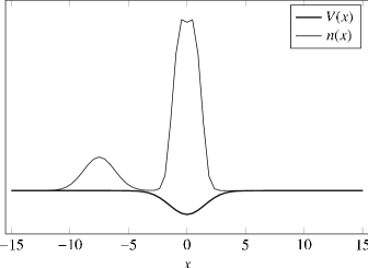
Figure 2: Particle density $n(x)$ of initial wavefunction and Gaussian well $V(x)$. Units are arbitrary.

The spatial particle density $n(x)=n(x,-1/2)+n(x,+1/2)$ of $|\Psi\rangle$ is shown in Fig. 2 along with the confining potential. The density $n(x,s)$ is given by the diagonal of the reduced one-body density matrix $\gamma(x,s,x^{\prime},s^{\prime})$, viz,

$$\gamma({x,s,x^{\prime},s^{\prime}})=\langle\Psi|\boldsymbol{\psi}^{\dagger}(x,s)\boldsymbol{\psi}(x^{\prime},s^{\prime})|\Psi\rangle,$$

or in terms of the coefficients $\rho^{(1)}=[\rho^{q}_{p}]$ and the orbitals,

$$\gamma=\Phi\rho^{(1)}\Phi^{H}.$$ (32)

Having obtained the MCTDHF initial wavefunction, the OATDCCD initial condition is computed as follows. We first transform the orthonormal orbitals $\Phi$ to generate orthonormal so-called Brueckner orbitals $\Phi_{\text{B}}$. The wavefunction amplitudes are transformed accordingly. By definition [39], the Brueckner orbitals optimize the overlap with the reference determinant, which is actually equivalent to the convenient property that the singles amplitudes vanish identically, the so-called Brillouin–Brueckner theorem. We now have

$$|\Psi\rangle=\langle\phi_{\text{B}}|\Psi\rangle(1+A_{2}+A_{3}+\cdots)|\phi_{\text{B}}\rangle=\langle\phi_{\text{B}}|\Psi\rangle e^{T_{2}+T_{3}+\cdots}|\phi_{\text{B}}\rangle,$$ (33)

where $|\phi_{\text{B}}\rangle$ is the determinant that has maximum overlap with $|\Psi\rangle$. We now simply take the OATDCC orbitals to be $\Phi_{\text{B}}$ (and $\tilde{\Phi}=\Phi_{\text{B}}^{H}$), and let $T_{2}$ be as in Eqn. (33), i.e., we perform a projection in CC amplitude space.

It remains to define $\Lambda_{2}$. We note that for the MCTDHF limit of OATDCC, $\langle\tilde{\Psi}|=\langle\Psi|/\langle\Psi|\Psi\rangle$, which gives $\Lambda_{n}$ such that

$$\langle\tilde{\Psi}|e^{T_{2}^{\dagger}+T_{3}^{\dagger}+\cdots}=\langle\phi_{\text{B}}|(1+\Lambda_{1}+\Lambda_{2}+\cdots),$$

which is used to extract $\Lambda_{2}$ algebraically in the computer code.

We comment that the initial condition computed in this way only is a critical point of the coupled cluster energy to within an approximation, albeit a very good one. Alternatively, we could solve the CCD equations in the Brueckner basis, which gives very similar results.

We comment that the OATDCC counterpart of the density matrix (32) is

$$\gamma=\Phi\rho^{(1)}\tilde{\Phi}.$$ (34)

The density plot of the OATDCC initial condition is visually indistinguishable from the MCTDHF initial condition, so we do not plot it separately in Fig. 2.

VI.4 Results

Having obtained initial conditions, these are propagated in time with $\Delta t=0.005$ until $t=t_{\text{final}}=30$. The energy is conserved to a very high precision, see Fig. 3. The energy-conservation also improves with reduced time step, as is expected.

As discussed in Section II.2, expectation values may gain small imaginary parts. Along the CC computation we therefore monitor

$$f(t)=\sum_{s}\int|\operatorname{Im}n(x,s,t)|\mathrm{d}x.$$ (35)

In Fig. 3 $f(t)$ is displayed, and it is indeed a small number compared to the particle number $N=5$.

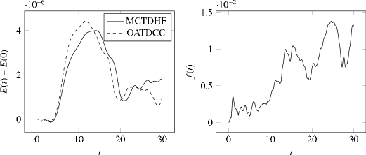
Figure 3: (Left) Energy conservation in the MCTDHF and OATDCCD schemes for the numerical experiment. The deviation from the initial energy is shown. The initial energies are $E_{\text{MCTDHF}}(0)=-12.2102145$ and $E_{\text{OATDCCD}}(0)=-12.2104173$. The gap between these numbers are due to neglection of the triples amplitudes and higher in the ground state. (Right) Integral of imaginary part of particle density, see Eqn. (35).

In Fig. 4 we show the density as function of $t$ of each calculation side by side. They are seen to agree qualitatively. The density evolution clearly shows how the incident electron interacts with the beryllium “atom”. Some of the density is clearly transmitted and reflected from the atom, while the atom is slightly perturbed, performing small amplitude oscillations. This demonstrates that manybody effects in the simulation are significant, and that the OATDCCD calculation captures these well.

Quantitatively, the densities show some differences after the collision event that may look like a phase shift in the oscillation of the atom part. We have not investigated further, but conjecture this to be a result of the fact that the CC approximation changes the spectrum slightly. The absolute value of the density difference is shown in Fig. 5.

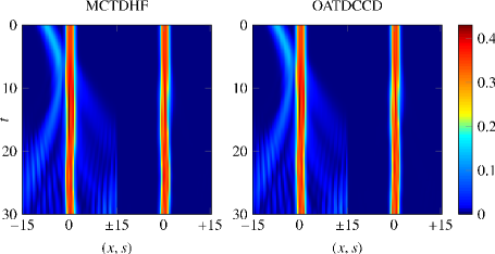
Figure 4: Electron density plot as function of time for each calculation. MCTDHF is on the left, while OATDCC is on the right. The $x$-axis is divided into spin up (left half) and spin down (right half). The two densities are seen to be very similar, see also Fig. 5. The incident electron is clearly reflected and partially transmitted through the initially stationary beryllium atom. After the collision, the atom is seen to exhibit oscillations. The interference fringes at the end of the simulations are due to boundary effects.

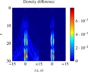
Figure 5: Differences between the OATDCC and MCTDHF electron densities calculated. The main feature is a phase-shift in the atom oscillations.

VII Conclusion

The bivariational principle for Schrödinger dynamics has been discussed at length, and the orbital-adaptive time-dependent coupled-cluster method (OATDCC) was developed. The method can be viewed as a systematic hierarchy of approximations to the highly successful multiconfigurational time-dependent Hartree method for fermions (MCTDHF), with simple time-dependent Hartree–Fock as the simplest case. The doubles approximation (OATDCCD) was discussed in detail, and numerical experiment performed showing that the method gives sensible results. OATDCC scales polynomially where MCTDHF scales exponentially with the number of particles $N$.

It was observed that imaginary time propagation for eigenvalue computation does not seem feasible for the OATDCC method. Studying methods for solving the time-independent orbital-adaptive CC should be a useful line of research. Such an eigenvalue computation method would constitute a hierarchy of approximations to the multiconfigurational Hartree–Fock method.

OATDCC is easily generalized to bosonic systems, with particularly interesting applications to Bose–Einstein condensates (BEC). The resulting method will approximate the MCTDH method for bosons [40], and can possibly treat substantially more particles. In fact, the CC approximation is very well suited to describe a BEC since it naturally captures the idea of excitations on top of a condensate.

Acknowledgments

The author wishes to thank Prof. Christian Lubich of Universität Tübingen, Germany, for fruitful discussions and Prof. Lars Bojer Madsen of Aarhus Universitet, Denmark, for constructive feedback on the manuscript. This work is supported by the DFG priority programme SPP-1324 [41]. Further financial support of CMA, University of Oslo, is gratefully acknowledged.

Appendix A Algebraic expressions for CCD

Here we list algebraic expressions for various quantities appearing in the OATDCC method using a doubles only ansatz, i.e., CCD. The expressions are computed using the second quantization toolbox in the Python library SymPy [22].

The expression for the expectation functional becomes

$$\mathcal{E}_{H}[\lambda,\tau,\tilde{\Phi},\Phi] =\langle\tilde{\phi}|He^{T}|\phi\rangle+\sum_{\mu}\lambda_{\mu}\frac{\partial}{\partial\lambda_{\mu}}\mathcal{E}_{H}[\lambda,\tau,\tilde{\Phi},\Phi]$$ (36)

$$=\langle\tilde{\phi}|He^{T}|\phi\rangle+\sum_{\mu}\lambda_{\mu}\langle\tilde{\phi}_{\mu}|e^{-T}He^{T}|\phi\rangle$$ (37)

$$=\langle\tilde{\phi}|He^{T}|\phi\rangle+\frac{1}{4}\sum_{ijab}\lambda_{ab}^{ij}\langle\tilde{\phi}_{ij}^{ab}|e^{-T}He^{T}|\phi\rangle$$ (38)

where we have used linearity of $\mathcal{E}_{H}$ in $\lambda_{\mu}$, and where the latter expression explicitly states the expansion in the CCD case.

To obtain computational formulae, we consider separately the one and two-body terms in $H$, i.e.,

$$H^{(1)}=\sum_{pq}h^{p}_{q}c^{\dagger}_{p}\tilde{c}_{q},\quad h^{p}_{q}=\langle\tilde{\varphi}_{p}|H^{(1)}|\varphi_{q}\rangle$$ (39)

and

$$H^{(2)}=\frac{1}{4}\sum_{pqrs}u^{pr}_{qs}c^{\dagger}_{p}c^{\dagger}_{r}\tilde{c}_{s}\tilde{c}_{q},\quad u^{pr}_{qs}=\langle\tilde{\varphi}_{p}\tilde{\varphi}_{r}|H^{(2)}|\varphi_{q}\varphi_{s}\rangle_{AS}$$ (40)

The coefficients $u^{pr}_{qs}$ are the the anti-symmetrized two-body integrals, see Equations (12) and (13). We get

$$\langle\tilde{\phi}|H^{(1)}e^{T}|\phi\rangle =h^{i}_{i}$$ (41a)

$$\langle\tilde{\phi}|H^{(2)}e^{T}|\phi\rangle =\frac{1}{4}\tau^{ab}_{ij}u^{ij}_{ab}+\frac{1}{2}u^{ij}_{ij}$$ (41b)

for the CCD energy, and

$$\frac{\partial}{\partial\lambda_{ab}^{ij}}\mathcal{E}_{H^{(1)}} =-h^{a}_{c}\tau^{bc}_{ij}P(ab)+h^{k}_{i}\tau^{ab}_{jk}P(ij)$$ (42a)

$$\frac{\partial}{\partial\lambda_{ab}^{ij}}\mathcal{E}_{H^{(2)}} =-\tau^{ab}_{ik}u^{kl}_{jl}P(ij)+\frac{1}{2}\tau^{ab}_{il}\tau^{dc}_{jk}u^{kl}_{dc}P(ij)+\frac{1}{4}\tau^{ab}_{kl}\tau^{dc}_{ij}u^{kl}_{dc}+\frac{1}{2}\tau^{ab}_{kl}u^{kl}_{ij}+\frac{1}{2}\tau^{ac}_{ij}\tau^{bd}_{kl}u^{kl}_{dc}P(ab)$$

$$+\tau^{ac}_{ij}u^{bk}_{ck}P(ab)-\tau^{ac}_{ik}\tau^{bd}_{jl}u^{kl}_{dc}P(ab)+\tau^{ac}_{ik}u^{bk}_{jc}P(ab)P(ij)+\frac{1}{2}\tau^{dc}_{ij}u^{ab}_{dc}+u^{ab}_{ij}$$ (42b)

for the derivatives with respect to $\lambda_{ab}^{ij}$. Inserting these expressions back into Eqn. (36), the complete expression for the CCD expectation value functional becomes

$$\mathcal{E}_{H}[\lambda,\tau,\tilde{\Phi},\Phi] =\frac{1}{2}h^{a}_{b}\lambda^{ij}_{ac}\tau^{bc}_{ij}+h^{i}_{i}-\frac{1}{2}h^{j}_{i}\lambda^{ki}_{ab}\tau^{ab}_{kj}-\frac{1}{2}\lambda^{ij}_{ab}\tau^{ab}_{ki}u^{kl}_{lj}+\frac{1}{8}\lambda^{ij}_{ab}\tau^{ab}_{kj}\tau^{dc}_{li}u^{kl}_{dc}$$ (43)

$$+\frac{1}{16}\lambda^{ij}_{ab}\tau^{ab}_{kl}\tau^{dc}_{ij}u^{kl}_{dc}+\frac{1}{8}\lambda^{ij}_{ab}\tau^{ab}_{kl}u^{kl}_{ij}+\frac{1}{8}\lambda^{ij}_{ab}\tau^{ab}_{li}\tau^{dc}_{kj}u^{kl}_{dc}+\frac{1}{2}\lambda^{ij}_{ab}\tau^{ac}_{ij}u^{bk}_{ck}$$ (44)

$$+\lambda^{ij}_{ab}\tau^{ac}_{ki}u^{bk}_{cj}-\frac{1}{2}\lambda^{ij}_{ab}\tau^{ac}_{kj}\tau^{db}_{li}u^{kl}_{dc}-\frac{1}{4}\lambda^{ij}_{ab}\tau^{ac}_{kl}\tau^{db}_{ij}u^{kl}_{dc}$$ (45)

$$+\frac{1}{8}\lambda^{ij}_{ab}\tau^{dc}_{ij}u^{ab}_{dc}+\frac{1}{4}\lambda^{ij}_{ab}u^{ab}_{ij}+\frac{1}{4}\tau^{ab}_{ij}u^{ij}_{ab}+\frac{1}{2}u^{ij}_{ij}$$ (46)

To solve the equations of motion for the amplitudes $\lambda_{ab}^{ij}$ we also need the derivatives of $\mathcal{E}_{H}$ with respect to $\tau_{ij}^{ab}$. For the one-body part

$$\frac{\partial}{\partial\tau_{ij}^{ab}}\mathcal{E}_{H^{(1)}}=h^{i}_{k}\lambda^{jk}_{ab}P(ij)-h^{c}_{a}\lambda^{ij}_{bc}P(ab),$$ (47a)

and for the two-body part,

$$\frac{\partial}{\partial\tau_{ij}^{ab}}\mathcal{E}_{H^{(2)}} =-\frac{1}{2}\lambda^{ij}_{bc}\tau^{dc}_{kl}u^{kl}_{ad}P(ab)-\lambda^{ij}_{bc}u^{ck}_{ak}P(ab)+\frac{1}{4}\lambda^{ij}_{dc}\tau^{dc}_{kl}u^{kl}_{ab}$$

$$+\frac{1}{2}\lambda^{ij}_{dc}u^{dc}_{ab}+\frac{1}{2}\lambda^{jk}_{ab}\tau^{dc}_{kl}u^{il}_{dc}P(ij)+\lambda^{jk}_{ab}u^{il}_{kl}P(ij)-\lambda^{jk}_{bc}\tau^{dc}_{kl}u^{il}_{ad}P(ab)P(ij)$$

$$+\lambda^{jk}_{bc}u^{ic}_{ak}P(ab)P(ij)+\frac{1}{2}\lambda^{jk}_{dc}\tau^{dc}_{kl}u^{il}_{ab}P(ij)+\frac{1}{4}\lambda^{kl}_{ab}\tau^{dc}_{kl}u^{ij}_{dc}+\frac{1}{2}\lambda^{kl}_{ab}u^{ij}_{kl}$$

$$-\frac{1}{2}\lambda^{kl}_{bc}\tau^{dc}_{kl}u^{ij}_{ad}P(ab)+u^{ij}_{ab}$$ (47b)

The operator $P(ij)$ is an anti-symmetrizer: $f(ij)P(ij)=f(ij)-f(ji)$, and similarly for $P(ab)$. The appearance of a $P(ij)$ or a $P(ab)$ should be ignored for the invocation of the summation convention.

Our calculations for expectation values and derivatives are of course valid for any one- or two-body operator.

Expressions for the reduced density matrices $\rho^{q}_{p}$ are readily obtained from $\mathcal{E}_{H^{(1)}}$ by using $h^{p^{\prime}}_{q^{\prime}}=\delta^{p^{\prime}}_{p}\delta_{q^{\prime}}^{q}$. We get $\rho^{a}_{i}=\rho^{i}_{a}=0$, while

$$\rho^{j}_{i} =\mathcal{E}_{c^{\dagger}_{i}\tilde{c}_{j}}=\delta^{k}_{i}\delta_{k}^{j}-\frac{1}{2}\delta^{l}_{i}\delta^{j}_{m}\lambda^{kl}_{ab}\tau^{ab}_{km}=\delta^{j}_{i}-\frac{1}{2}\lambda^{kj}_{ab}\tau^{ab}_{ki}$$ (48a)

$$\rho^{b}_{a} =\mathcal{E}_{c^{\dagger}_{a}\tilde{c}_{b}}=\frac{1}{2}\delta^{d}_{a}\delta^{b}_{e}\lambda^{ij}_{dc}\tau^{ec}_{ij}=\frac{1}{2}\lambda^{ij}_{ac}\tau^{bc}_{ij}$$ (48b)

Finally, we compute the two-body reduced density matrix. We only list nonzero elements.

$$\rho^{kl}_{ij} =P(ij)\delta^{k}_{i}\delta^{l}_{j}-P(ij)P(kl)\frac{1}{2}\delta^{k}_{i}\lambda^{lm}_{cd}\tau^{cd}_{jm}+\frac{1}{2}\lambda^{kl}_{cd}\tau^{cd}_{ij}$$ (49a)

$$\rho^{ab}_{ij} =-P(ab)\frac{1}{2}\lambda^{kl}_{cd}\tau^{ac}_{ij}\tau^{bd}_{kl}+P(ij)\lambda^{kl}_{cd}\tau^{ac}_{ik}\tau^{bd}_{jl}$$

$$\qquad+P(ij)\frac{1}{2}\lambda^{kl}_{cd}\tau^{ab}_{il}\tau^{cd}_{jk}+\frac{1}{4}\lambda^{kl}_{cd}\tau^{ab}_{kl}\tau^{cd}_{ij}+\tau^{ab}_{ij}$$ (49b)

$$\rho^{jb}_{ia} =-\rho^{bj}_{ia}=-\rho^{jb}_{ai}=\rho^{bj}_{ai}=\frac{1}{2}\delta^{j}_{i}\lambda^{kl}_{ac}\tau^{bc}_{kl}-\lambda^{jk}_{ac}\tau^{bc}_{ik}$$ (49c)

$$\rho^{ij}_{ab} =\lambda^{ij}_{ab}$$ (49d)

$$\rho^{cd}_{ab} =\frac{1}{2}\lambda^{ij}_{ab}\tau^{cd}_{ij}$$ (49e)

Appendix B Derivation of MCTDHF

The purpose of this section is to provide a brief derivation of the MCTDHF method independently of the existing derivations in the literature, using the time-dependent bivariational principle.

The bivariational MCTDHF manifold is

$$\mathcal{M}_{\text{MCTDHF}}=\bigcup_{\tilde{\Phi}\Phi=I}\tilde{\mathcal{V}}[\tilde{\Phi}]\times\mathcal{V}[\Phi],$$ (50)

where the union is taken over all biorthogonal choices of orbitals. That is to say, $|\Psi\rangle$ is an arbitrary vector in the discrete (FCI) Hilbert space generated by $\Phi$, and $\langle\tilde{\Psi}|$ is an arbitrary vector in the discrete space generated by the dual orbitals $\tilde{\Phi}$:

$$|\Psi\rangle =\sum_{\mu}A^{\mu}|\phi_{\mu}\rangle$$ (51)

$$\langle\tilde{\Psi}| =\sum_{\mu}\tilde{A}_{\mu}\langle\tilde{\phi}^{\mu}|,$$ (52)

where we include the reference determinants in the sums by defining $|\phi_{0}\rangle\equiv|\phi\rangle$ and $\langle\tilde{\phi}_{0}|\equiv\langle\tilde{\phi}|$, i.e., $\mu=0$ is the reference. Since the FCI spaces are linear it is allowed to remove the phase and normalization ambiguity in Eqn. (4) by requiring $\langle\tilde{\Psi}|\Psi\rangle=1$.

The time derivative of $|\Psi\rangle$ is

$$\frac{\partial}{\partial t}|\Psi\rangle=\sum_{\mu}\dot{A}^{\mu}|\phi_{\mu}\rangle+D|\Psi\rangle,$$ (53)

where $D$ is defined in Eqn. (17). We obtain two expressions for the action functional, which are equivalent:

$$\mathcal{S}[\tilde{A},A,\tilde{\Phi},\Phi] =\int_{0}^{T}\mathrm{i}\hbar\tilde{A}_{\mu}\dot{A}^{\mu}+\mathrm{i}\hbar\tilde{A}_{\mu}D^{\mu}_{\nu}A^{\nu}-\tilde{A}_{\mu}H^{\mu}_{\nu}A^{\nu}\;\mathrm{d}t$$ (54)

$$=\int_{0}^{T}\mathrm{i}\hbar\tilde{A}_{\mu}\dot{A}^{\mu}+\rho^{q}_{p}(\mathrm{i}\hbar\eta^{p}_{q}-h^{p}_{q})-\frac{1}{4}\rho^{qs}_{pr}u^{pr}_{qs}\;\mathrm{d}t,$$ (55)

where

$$D^{\mu}_{\nu}\equiv\langle\tilde{\phi}^{\mu}|D|\phi_{\nu}\rangle,\quad H^{\mu}_{\nu}\equiv\langle\tilde{\phi}^{\mu}|H||\phi_{\nu}\rangle,\quad\eta^{p}_{q}\equiv\langle\tilde{\varphi}_{p}|\dot{\varphi}_{q}\rangle,$$ (56)

and where

$$\rho^{q}_{p}\equiv\langle\tilde{\Psi}|c^{\dagger}_{p}\tilde{c}_{q}|\Psi\rangle,\quad\rho^{qs}_{pr}\equiv\langle\tilde{\Psi}|c^{\dagger}_{p}c^{\dagger}_{r}\tilde{c}_{s}\tilde{c}_{q}|\Psi\rangle$$ (57)

are the reduced one- and two-body density matrices.

In a similar way as for the CC ansatz, it can be shown that mixing of the orbitals $\Phi\rightarrow\Phi G$ and $\tilde{\Phi}\rightarrow G^{-1}\tilde{\Phi}$, $G$ being an arbitrary invertible $L\times L$ matrix, with a corresponding inverse operation on $A$ and $\tilde{A}$ leaves the action invariant (except for a total time derivative with vanishing variation). This implies that all the inner products $\eta^{p}_{q}$ can be chosen arbitrarily, and we choose $\eta^{p}_{q}\equiv 0$ for simplicity, which implies $D^{\mu}_{\nu}\equiv 0$. This corresponds to the usual gauge choice in MCTDHF theory, see Ref. [2]. The resulting permissible variations in $\varphi_{p}$ are then of the form $\delta\varphi_{p}=\chi=Q\chi$, with $Q=1-\Phi\tilde{\Phi}$. Similarly, the permissible variations in $\tilde{\varphi}_{p}$ are $\delta\tilde{\varphi}_{p}=\tilde{\chi}=\tilde{\chi}Q$. The $P$-space variations are identically zero in this gauge.

Performing first the variations in $\tilde{A}_{\nu}$ and $A^{\mu}$, respectively, we obtain the equations

$$\mathrm{i}\hbar\dot{A}^{\nu}=H^{\nu}_{\mu}A^{\mu}\quad\text{and}\quad-\mathrm{i}\hbar\dot{\tilde{A}}_{\mu}=\tilde{A}_{\nu}H^{\nu}_{\mu},$$ (58)

i.e., the time-dependent Schrödinger equation in a moving basis and its dual equation. Since $H^{\nu}_{\mu}=\langle\tilde{\phi}^{\nu}|\Pi H\Pi|\phi_{\mu}\rangle$, the operator expression (11) is useful for implementations.

Performing the variations in $\tilde{\varphi}_{p}$ we obtain, in a manner similar to Section IV.2, the equation

$$\mathrm{i}\hbar\sum_{q}\rho^{q}_{p}|\dot{\varphi}_{q}\rangle=Q\left[\sum_{q}\rho^{q}_{p}h|\varphi_{q}\rangle+\sum_{qrs}\rho^{qs}_{pr}W^{r}_{s}|\varphi_{q}\rangle\right],$$ (59)

and performing the variation in $\varphi_{q}$ we obtain

$$-\mathrm{i}\hbar\sum_{p}\rho^{q}_{p}\langle\dot{\tilde{\varphi}}_{p}|=\left[\sum_{p}\rho^{q}_{p}\langle\tilde{\varphi}_{p}|h+\sum_{prs}\rho^{qs}_{pr}\langle\varphi_{p}|W^{r}_{s}\right]Q,$$ (60)

which are identical in form to Eqns. (30e) and (30f).

Assume now that $\tilde{\Phi}(0)=\Phi(0)^{H}$ at time $t=0$, and that $\tilde{A}_{\mu}(0)=A^{\mu}(0)^{*}$. Then clearly $\rho^{q}_{p}=(\rho_{q}^{p})^{*}$ and $\rho^{qs}_{pr}=(\rho^{pr}_{qs})^{*}$. Similarly, $h^{p}_{q}=(h^{q}_{p})^{*}$ and $u^{pr}_{qs}=(u^{qs}_{pr})^{*}$.

From this it follows that $\langle\dot{\tilde{\varphi}}_{p}|=|\dot{\varphi}_{p}\rangle^{\dagger}$, $\dot{\tilde{A}}_{\mu}=(\dot{A}^{\mu})^{*}$ and hence $\langle\tilde{\Psi}(t)|=|\Psi(t)\rangle^{\dagger}$ for all $t$.

Comparing with the equations of motion in, say, Ref. [42], we see that we indeed have arrived at the MCTDHF equations of motion.

Appendix C Some techinical proofs

C.1 Orbital transformations

We consider the orbital transformation

$$\Phi\longrightarrow\Phi^{\prime}=\Phi G,\quad\tilde{\Phi}\longrightarrow\tilde{\Phi}^{\prime}=G^{-1}\tilde{\Phi},$$ (61)

where $G=\exp(g)$ is an $L\times L$ invertible matrix. (Recall that any invertible matrix has a logarithm.) The transformation preserves biorthogonality. The transformation is equivalent to transforming the creation and annihilation operators as

$$c^{\dagger}_{p}\longrightarrow\sum_{q}c^{\dagger}_{q}G_{qp},\quad\tilde{c}_{p}\longrightarrow\sum_{q}G^{-1}_{pq}\tilde{c}_{q}.$$ (62)

We wish to show, that Eqn. (62) is again equivalent to

$$c^{\dagger}_{p}\longrightarrow e^{\hat{g}}c^{\dagger}_{p}e^{-\hat{g}},\quad\tilde{c}_{q}\longrightarrow e^{\hat{g}}\tilde{c}_{q}e^{-\hat{g}},$$ (63)

where

$$\hat{g}=\sum_{pq}g_{qp}c^{\dagger}_{q}\tilde{c}_{p}.$$ (64)

We begin by noting that the similarity transform can be expanded using the BCH formula as

$$e^{\hat{g}}xe^{-\hat{g}}=x+[\hat{g},x]+\frac{1}{2!}[\hat{g},[\hat{g},x]]+\cdots=\sum_{n=0}^{\infty}\frac{1}{n!}[\hat{g},x]_{n}$$ (65)

where $[A,B]_{n}$ is the $n$-fold nested commutator. Suppose we can show, that for all $n\geq 0$,

$$[\hat{g},c^{\dagger}_{p}]_{n} =\sum_{q}(g^{n})_{qp}c^{\dagger}_{q},$$ (66a)

and

$$[\hat{g},\tilde{c}_{q}]_{n} =\sum_{p}(-1)^{n}(g^{n})_{qp}\tilde{c}_{p}.$$ (66b)

This would imply

$$e^{\hat{g}}c^{\dagger}_{p}e^{-\hat{g}} =\sum_{n=0}^{\infty}\frac{1}{n!}\sum_{q}(g^{n})_{qp}c^{\dagger}_{q}=\sum_{q}G_{qp}c^{\dagger}_{q}$$ (67)

and

$$e^{\hat{g}}\tilde{c}_{q}e^{-\hat{g}} =\sum_{n=0}^{\infty}\frac{(-1)^{n}}{n!}\sum_{p}(g^{n})_{qp}\tilde{c}_{p}=\sum_{p}G^{-1}_{qp}\tilde{c}_{p},$$ (68)

which would prove the result.

We prove Eqn. (66) by induction, and for simplicity we consider only (66a). The proof for (66b) is similar. For $n=0$, $(g^{0})_{qp}=\delta_{qp}$, which shows that $n=0$ is trivially true. Suppose now, that Eqn. (66a) holds for some $n\geq 0$. We show that it holds for $n+1$ as well. We get

$$[\hat{g},c^{\dagger}_{q}]_{n+1}=[\hat{g},[\hat{g},c^{\dagger}_{q}]_{n}]=[\hat{g},\sum_{r}g^{n}_{rq}c^{\dagger}_{r}]=\sum_{psr}g_{sp}g^{n}_{rq}[c^{\dagger}_{s}\tilde{c}_{p},c^{\dagger}_{r}]=\sum_{psr}g_{sp}g^{n}_{rq}\delta_{pr}c^{\dagger}_{s}=\sum_{s}g^{n+1}_{sp}c^{\dagger}_{s},$$ (69)

which proves the induction step. We have used that

$$[c^{\dagger}_{s}\tilde{c}_{p},c^{\dagger}_{r}]=\delta_{pr}c^{\dagger}_{s},$$ (70)

which is easily calculated using the fundamental anticommutator.

C.2 Amplitude equations

In this section, we consider the derivation of the amplitude equations (24) from the variation of the OATDCC functional with respect to the amplitudes $\lambda_{\mu}$ and $\tau^{\mu}$, which are all independent variables. We therefore start with varying a single amplitude $\lambda_{\nu}(t)$, i.e., $\delta\lambda_{\mu}(t)=0$ for $\mu\neq\nu$, and $\delta\tau^{\mu}(t)=0$ for all $\mu\in\mathcal{I}$. Note that all variations vanish at the end points $t=0$ and $t=T$ of the time interval. We wish to compute

$$\delta\mathcal{S}[\lambda,\tau]=\delta\int_{0}^{T}\mathrm{i}\hbar\lambda_{\mu}(t)\dot{\tau}^{\mu}(t)-\mathcal{E}_{H-\mathrm{i}\hbar D_{0}}[\lambda(t),\tau(t)]\;\mathrm{d}t,$$ (71)

where we have suppressed the dependence on $\tilde{\Phi}$ and $\Phi$ in $\mathcal{E}$ and $\mathcal{S}$ since they are held fixed in the variation. We obtain

$$\delta\mathcal{S}[\lambda,\tau] =\int_{0}^{T}\mathrm{i}\hbar\delta\lambda_{\nu}(t)\dot{\tau}^{\nu}-\frac{\partial\mathcal{E}_{H-\mathrm{i}\hbar D_{0}}[\lambda(t),\tau(t)]}{\partial\lambda_{\nu}}\delta\lambda_{\nu}(t)\;\mathrm{d}t$$ (72)

$$=\int_{0}^{T}\delta\lambda_{\nu}(t)\left[\mathrm{i}\hbar\dot{\tau}^{\nu}-\frac{\partial\mathcal{E}_{H-\mathrm{i}\hbar D_{0}}[\lambda(t),\tau(t)]}{\partial\lambda_{\nu}}\right]\;\mathrm{d}t=0.$$ (73)

Note that we do not invoke the summation convention. Since the expression must vanish for all choices of $\lambda_{\nu}(t)$, it follows that

$$\mathrm{i}\hbar\dot{\tau}^{\nu}(t)=\frac{\partial}{\partial\lambda_{\nu}}\mathcal{E}_{H-\mathrm{i}\hbar D_{0}}[\lambda(t),\tau(t),\tilde{\Phi}(t),\Phi(t)]$$ (74)

must hold.

Similarly, we hold $\lambda_{\mu}$ fixed, and vary only a single amplitude $\tau^{\nu}$.

$$\delta\mathcal{S}[\lambda,\tau] =\int_{0}^{T}\mathrm{i}\hbar\lambda_{\nu}(t)\delta\dot{\tau}^{\nu}-\frac{\partial\mathcal{E}_{H-\mathrm{i}\hbar D_{0}}[\lambda(t),\tau(t)]}{\partial\tau^{\nu}}\delta\tau^{\nu}(t)\;\mathrm{d}t$$ (75)

$$=\int_{0}^{T}\delta\tau^{\nu}(t)\left[-\mathrm{i}\hbar\dot{\lambda}_{\nu}-\frac{\partial\mathcal{E}_{H-\mathrm{i}\hbar D_{0}}[\lambda(t),\tau(t)]}{\partial\tau^{\nu}}\right]\;\mathrm{d}t+\mathrm{i}\hbar\left[\lambda_{\nu}(t)\delta\tau^{\nu}(t)\right]_{t=0}^{T}$$ (76)

where we have performed integration by parts. The boundary terms vanish by definition of the variation, so that we get

$$-\mathrm{i}\hbar\dot{\lambda}_{\nu}(t)=\frac{\partial}{\partial\tau^{\nu}}\mathcal{E}_{H-\mathrm{i}\hbar D_{0}}[\lambda(t),\tau(t),\tilde{\Phi}(t),\Phi(t)].$$ (77)

References

- [1] H.-D. Meyer, F. Gatti, and G. A. Worth, editors. Multidimensional Quantum Dynamics: MCTDH Theory and Applications. Wiley, 2009.
- [2] M. H. Beck, A. Jäckle, G.A. Worth, and H.-D. Meyer. The multiconfiguration time-dependent Hartree (MCTDH) method: a highly efficient algorithm for propagating wavepackets. Phys. Rep., 324(1):1–105, 2000.
- [3] H.-D. Meyer, U. Manthe, and L. S. Cederbaum. The multi-configurational time-dependent Hartree approach. Chem. Phys. Lett., 165(1):73 – 78, 1990.
- [4] J. Broeckhove, L. Lathouwers, E. Kesteloot, and P. Van Leuven. On the equivalence of time-dependent variational principles. Chem. Phys. Lett., 149(5-6):547–550, 1988.
- [5] P. Kramer and M. Saraceno. Geometry of the time-dependent variational principle. Springer, 1981.
- [6] C. Lubich. On variational approximations in quantum molecular dynamics. Math. Comp., 74:765–779, 2005.
- [7] J. Zanghellini, M. Kitzler, T. Brabec, and T. Scrinzi. Testing the multi-configuration time-dependent hartree-fock method. J. Phys. B: At. Mol. Opt. Phys., 37(4):763, 2004.
- [8] T. Helgaker, P. Jørgensen, and J. Olsen. Molecular Electronic-Structure Theory. Wiley, 2002.
- [9] I. Shavitt and R. J. Bartlett. Many-body methods in chemistry and physics: MBPT and Coupled-Cluster Theory. Cambridge, 2009.
- [10] J. Arponen. Variational principles and linked-cluster exp s expansions for static and dynamic many-body problems. Annals of Physics, 151(2):311–382, 1983.
- [11] E. Dalgaard and H. J. Monkhorst. Some aspects of the time-dependent coupled-cluster approach to dynamic response functions. Phys. Rev. A, 28(3):1217–1222, Sep 1983.
- [12] T. Helgaker and P. Jørgensen. Configuration-interaction energy derivatives in a fully variational formulation. Theor. Chim. Acta, 75:111–127, 1989. 10.1007/BF00527713.
- [13] H. Koch and P. Jørgensen. Coupled cluster response functions. J. Chem. Phys., 93(5):3333–3344, 1990.
- [14] T. Bondo Pedersen, B. Fernandez, and H. Koch. Gauge invariant coupled cluster response theory using optimized nonorthogonal orbitals. J. Chem. Phys., 114(16):6983–6993, 2001.
- [15] T. D. Crawford. An Introduction to Coupled Cluster Theory for Computational Chemists. Rev. Comp. Chem., 14:33–126, 2000.
- [16] R. J. Bartlett and M. Musiał. Coupled-cluster theory in quantum chemistry. Rev. Mod. Phys., 79(1):291, 2007.
- [17] F.E. Harris, H. Monkhorst, and D.L. Freeman. Algebraic and Diagrammatic Methods in Many-Fermion Theory. Oxford, 1992.
- [18] K. Schönhammer and O. Gunnarsson. Time-dependent approach to the calculation of spectral functions. Phys. Rev. B, 18(12):6606–6614, Dec 1978.
- [19] P. Hoodbhoy and J. W. Negele. Time-dependent coupled-cluster approximation to nuclear dynamics. I. Application to a solvable model. Phys. Rev. C, 18(5):2380–2394, Nov 1978.
- [20] P. Hoodbhoy and J. W. Negele. Time-dependent coupled-cluster approximation to nuclear dynamics. II. General formulation. Phys. Rev. C, 19(5):1971–1982, Apr 1979.
- [21] C. Huber and T. Klamroth. Explicitly time-dependent coupled cluster singles doubles calculations of laser-driven many-electron dynamics. J. Chem. Phys., 134:054113, 2011.
- [22] SymPy Development Team. SymPy: Python library for symbolic mathematics, 2009.
- [23] Reinhold Schneider. Analysis of the projected coupled cluster method in electronic structure calculation. Numer. Math., 113:433–471, 2009. 10.1007/s00211-009-0237-3.
- [24] T. Rohwedder. The continuous coupled cluster formulation for the electronic SchrÖdinger equation. Submitted to M2AN, 2011.
- [25] T. Rohwedder and R. Schneider. Error estimates for the coupled cluster method. Submitted to M2AN, 2011.
- [26] O. Koch and C. Lubich. Regularity of the multi-configuration time-dependent Hartree approximation in quantum molecular dynamics. ESAIM: Mathematical Modelling and Numerical Analysis, 41(2):315–331, MAR-APR 2007.
- [27] D. Conte and C. Lubich. An error analysis of the multi-configuration time-dependent Hartree method of quantum dynamics. Mathematical Modelling and Numerical Analysis, 44:759–780, 2010.
- [28] C. Bardos, I. Catto, N. Mauser, and S. Trabelsi. Setting and Analysis of the Multi-configuration Time-dependent Hartree-Fock Equations. Arch. Rat. Mech. Anal., 198(1):273–330, OCT 2010.
- [29] P.-O. Löwdin, P. Froelich, and M. Mishra. Some properties of the bivariational hartree-fock scheme for complex symmetric many-particle operators. Int. J. Quant. Chem., 36(2):93–103, 1989.
- [30] J. Killingbeck. Quantum-mechanical perturbation theory. Rep. Prog. Phys, 40:963–1031, 1977.
- [31] G. C. Wick. The evaluation of the collision matrix. Phys. Rev., 80:268–272, Oct 1950.
- [32] W. Kutzelnigg. Error analysis and improvements of coupled-cluster theory. Theor. Chim. Acta, 80(4-5):349–386, OCT 1991.
- [33] S. Hirata. Symbolic Algebra in Quantum Chemistry. Theor. Chim. Acta, 116:2–17, 2006. 10.1007/s00214-005-0029-5.
- [34] H.J. Monkhorst. Calculation of properties with coupled-cluster method. Int. J. Quant. Chem., 12(Y-11):421–432, 1977.
- [35] C. Lubich. From Quantum to Classical Molecular Dynamics: Reduced Models and Numerical Analysis. European Mathematical Society, 2008.
- [36] S. M. Reimann and M. Manninen. Electronic structure of quantum dots. Rev. Mod. Phys, 74:1283–1342, 2002.
- [37] H. Tal-Ezer and R. Kosloff. An accurate and efficient scheme for propagating the time dependent schr[o-umlaut]dinger equation. J. Chem. Phys., 81(9):3967–3971, 1984.
- [38] O. Koch and C. Lubich. Variational-splitting time integration of the multi-configuration time-dependent Hartree-Fock equations in electron dynamics. IMA J. Numer. Anal., 31:379–395, 2011.
- [39] P.-O. Löwdin. Studies in Perturbation Theory. V. Some Aspects on the Exact Self-Consistent Field Theory. J. Math. Phys., 3(6):1171–1184, 1962.
- [40] O. E. Alon, A. I. Streltsov, and L. S. Cederbaum. Multiconfigurational time-dependent Hartree method for bosons: Many-body dynamics of bosonic systems. Phys. Rev. A, 77(3):033613, Mar 2008.
- [41] Web page of DFG priority program 1324. http://www.dfg-spp1324.de. Accessed: 26/01/2012.
- [42] J. Zanghellini, M. Kitzler, Ch. Fabian, T. Brabec, and A. Scrinzi. A MCTDHF approach to multi-electron dynamics in laser fields. Laser Physics, 13:1064–1068, 2003.