Reacting particles in open chaotic flows

Abstract

We study the collision probability $p$ of particles advected by open flows displaying chaotic advection. We show that $p$ scales with the particle size $\delta$ as a power law whose coefficient is determined by the fractal dimensions of the invariant sets defined by the advection dynamics. We also argue that this same scaling also holds for the reaction rate of active particles in the low-density regime. These analytical results are compared to numerical simulations, and we find very good agreement with the theoretical predictions.

Many fluid flows of interest to science and to engineering are open flows, which are characterised by the presence of inflow and outflow regions batchelor (see Fig. 1a). The dynamics of advected particles in open flows is transient, with typical particles leaving to the outflow region in finite time. Advection in many open flows is chaotic Jung-et-al-93 ; Tel-et-al-05 ; examples of chaotic open flows are found in areas such as microfluidics Strook2002 , climatology Koh2002 , physiology Schelin2009 , population biology Karolyi2000 and industry Gouillart2009a ; Gouillart2011measures . The dynamics of advected particles is governed by the chaotic saddle cscatbook , which is a set of unstable orbits contained in a bounded region of space known as the mixing region (see Fig. 1a). Fluid elements are repeatedly stretched and folded in the mixing region, and this causes any portion of the fluid to be deformed by the flow into a complex filamentary shape, which shadows the unstable manifold of the chaotic saddle, defined as the fractal set of orbits which converge asymptotically to the chaotic saddle for $t\rightarrow-\infty$ cscatbook .

The fractal structures generated by chaotic advection have dramatic consequences for the dynamics of active processes taking place in open flows, such as chemical reactions and biological processes Tel-et-al-05 . The stretching and folding of fluid elements by the flow tends to increase the area (or perimeter, in 2D flows) of contact between two reacting species, which results in an enhancement of the reaction due purely to the advective dynamics of the flow—this has been called dynamic catalysis Tel-et-al-05 . It has been shown Karolyi1999 ; Tel-et-al-05 that this effect appears as a singular production term in an effective reaction rate equation, which has a power-law dependence on the amount of reactant; the coefficient of the power law is determined by the information fractal dimension of the unstable manifold of the chaotic saddle. Later works have established that this enhancement of activity by chaos is a very general and robust phenomenon Tel-et-al-05 , and is a feature of many kinds of activity and flows, including non-periodic Karolyi2004 , non-hyperbolic Motter2003 ; Moura2004 and three-dimensional Moura2004b flows.

All the works so far on the effects of chaos on chemical or biological activity in open flows have adopted continuum descriptions of the reacting material — either describing the reactants using continuous concentration fields, or modelling the propagation of the reaction through reaction fronts. This approach ignores the fact that any activity taking place in the fluid ultimately arises from collisions of particles. If the number of reacting particles is very large, so that the mean free path between collisions is much smaller than the typical length scale of the system, then this continuous description is expected to be valid. However, in the low-density limit, where typically particles traverse large distances before colliding and reacting, the concepts of reactant concentration and reaction front have no meaning. In this case, one must adopt a kinetic theory approach, where activity is described in terms of the probability of collision between particles. Although this idea has been used in closed flows — in the context of chemical catalysis Metcalfe1994 , particle coalescence Nishikawa2001 ; Springer2010 and crystallisation Cartwright2004 , for example — so far this idea has not been pursued in the case of open flows, despite the importance of the low-density regime for applications, which is appropriate for describing systems as diverse as platelet activation in blood flows Schelin2009 , plankton population dynamics Karolyi2004 , and raindrop formation Wilkinson2006 ; Vilela2007 .

In this work we investigate the effect of chaotic advection on the activity of particles in the low-density limit. The rate of reaction in this limit is determined by the collision probability $p(\delta)$ of two particles coming within a distance $\delta$ of each other before they escape to the outflow; we assume a reaction event takes place when that happens. $\delta$ can be thought of as the size of the particles, or alternatively as determined by the reaction cross-section $\sigma$ (with $\delta\sim\sqrt{\sigma}$). We show that $p$ scales with $\delta$ as a power law, $p(\delta)\sim\delta^{\beta}$, and we derive an analytical expression for the coefficient $\beta$ in terms of the fractal dimensions of the stable and unstable manifolds of the chaotic saddle. The classical kinetic theory approach, based on the Smoluchowski equation Smoluchowski1916 , which assumes there is a homogeneous mixing of particles in the mixing region, would predict $\beta=N$, where $N$ is the spatial dimension, but we show that because most collisions happen in the neighbourhood of a fractal set, Smoluchowski’s result does not hold, and $\beta\neq N$ for open chaotic flows. In the low-density limit, the total number $Q(\delta)$ of reaction events between reacting particle species which takes place in a given flow also scales as $\delta^{\beta}$. We argue that $Q$ is a good measure of the efficiency of mixing in open flows, and thus $\beta$ characterises the mixing of an open flow. These analytical predictions are compared to numerical simulations in 2D flows, and we find the results agree very well with our theory.

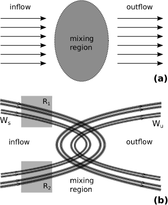
Figure 1: (a) Illustration of an open flow. (b) Schematic depiction of the stable ($W_{s}$) and unstable ($W_{u}$) manifolds in an open flow. The grey bands are $\delta$-neighbourhoods of $W_{s}$ and $W_{u}$ (see text). $R_{1}$ and $R_{2}$ indicate regions where initial conditions are chosen.

We start by deriving the scaling of the collision probability $p(\delta)$ of two particles with randomly chosen initial conditions, by first assuming that after the particles enter the mixing region (Fig. 1a), the flow acts as a perfect, uniform mixer, until the particles escape to the outflow. This perfect mixing assumption means that the positions of the two particles are effectively randomised in a time interval $\tau$ which is characteristic of the flow. The probability that two particles randomly placed in a bounded $N$-dimensional region are within a distance $\delta$ of each other scales as $\delta^{N}$. Assuming that $\delta$ is small enough so that the probability $p(\delta)$ that the two particles collide before escaping satisfies $p(\delta)\ll 1$, we conclude that $p(\delta)$ is proportional to $\delta^{N}$ and to the average time $T$ the particle stays in the mixing region before escaping. $p(\delta)$ therefore scales with $\delta$ as

$$p(\delta)\sim\delta^{N},$$ (1)

The perfect mixing assumption is the assumption used in Smoluchowski’s classical coagulation theory Smoluchowski1916 , and we will refer to this $\delta^{N}$ scaling as the Smoluchowski prediction.

The Smoluchowski scaling derived above does not take into account the fractal nature of the particle distributions generated by chaotic advection in open flows. We will now derive the correct scaling of $p(\delta)$. Let two particles be chosen randomly within two bounded and disjoint regions $R_{1}$ and $R_{2}$ (see Fig. 1b). As a result of the chaotic dynamics of the flow in the mixing region, those trajectories which take longer to escape converge towards the unstable manifold $W_{u}$. Consequently, the particles will only have a chance to meet if both come within a distance $\delta$ (the reaction distance) of the unstable manifold. This will take place if their initial conditions are within a distance of order $\delta$ of the stable manifold $W_{s}$, which is the set of initial conditions converging to the chaotic saddle for $t\rightarrow\infty$ (see Fig. 1b) cscatbook . The probability $P_{s}^{(1)}(\delta)$ that one particle with initial conditions in $R_{1}$ lies within a distance of order $\delta$ of the stable manifold is proportional to the volume $V_{1}$ (or area in two dimensions) of the intersection of $R_{1}$ and a $\delta$-covering of the component of $W_{s}$ where the conditionally invariant measure is concentrated Grassberger1983 ; cscatbook (see Fig. 1b). If one imagines $R_{1}$ to be covered by a grid of size $\delta$, the number of cells in the grid intersecting the component of $W_{s}$ where the conditionally invariant measure is concentrated scales as $N_{1}(\delta)\sim\delta^{-D_{1}^{s}}$ cscatbook , where $D_{1}^{s}$ is the information dimension of the stable manifold. Since the volume of each cell in the grid is $\delta^{N}$, the volume of the portion of the grid which intersects $W_{s}$ scales as $V_{1}\sim N(\delta)\delta^{N}\sim\delta^{N-D_{1}^{s}}$. We therefore have $P_{s}^{(1)}(\delta)\sim\delta^{N-D_{1}^{s}}$, and the same scaling holds for the probability $P_{s}^{(2)}$ that the other particle is close to $W_{s}$. Therefore, the probability $P_{s}=P_{s}^{(1)}P_{s}^{(2)}$ that both particles reach a $\delta$-neighbourhood of the unstable manifold scales as

$$P_{s}(\delta)\sim\delta^{2N-2D_{1}^{s}}.$$ (2)

The two particles collide if they reach the unstable manifold within a distance $\delta$ of each other. Considering again a grid of size $\delta$ covering the unstable manifold $W_{u}$, the probability $P_{u}(\delta)$ that two particles collide can be approximated by the probability that they end up in the same cell in the grid. This is given by $P_{u}(\delta)=\sum_{i}\mu_{i}^{2}$, where $\mu_{i}$ is the (conditionally invariant) measure of cell $i$, and the sum is over all cells intersecting the unstable manifold. From the definition of the correlation dimension $D_{2}^{u}$ Grassberger1983 ; cscatbook , we find that in the limit $\delta\rightarrow 0$ we get

$$P_{u}(\delta)\sim\delta^{D_{2}^{u}}.$$ (3)

The overall probability $p(\delta)=P_{s}(\delta)P_{u}(\delta)$ that the two particles will collide therefore scales as

$$p(\delta)\sim\delta^{\beta},\hskip 14.22636pt\text{with}\ \ \beta=2N-2D_{1}^{s}+D_{2}^{u}.$$ (4)

This is our main result. This scaling is clearly different from the Smoluchowski prediction: for chaotic flows, in general we expect $\beta\neq N$. However, $\beta$ does approach the Smoluchowski value of $N$ in the limit where the escape rate vanishes, when $D_{1}^{2},D_{2}^{u}\rightarrow N$, and from Eq. (4) this implies that $\beta\rightarrow N$. This behaviour is expected, since in this limit the dynamics within the mixing region can be considered as that of a closed container being stirred, with a small leak, when particles spend a long lime in the mixing region and the perfect mixing assumption is approximately valid.

The scaling predicted by Eq. (4) is valid for any choice of regions $R_{1}$ and $R_{2}$, as long as both regions intersect the stable manifold $W_{s}$. If there is no intersection, the two particles never meet because they do not get to the mixing region, and collisions cannot take place.

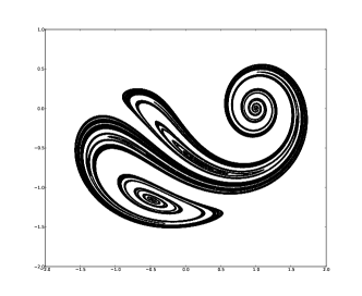
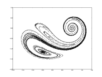
Figure 2: (a) Numerical approximation of the unstable manifold for the blinking vortex-sink flow, with $\eta=0.5$ and $\xi=10$; for these parameters, the dynamics is chaotic and hyperbolic. (b) Location of collisions for $\delta=10^{-3}$, for the flow with the same parameters as above. It is clear that collisions take place in the vicinity of the unstable manifold. The initial conditions were chosen in the regions $R_{1}$ ($-0.5<x<0.5$, $0<y<0.15$) and $R_{2}$ ($-0.5<x<0.5$, $0.2<y<0.35$). The time step used in the simulations was $\Delta t=0.02$.

To test the prediction of Eq. (4), we will use the blinking vortex-sink flow, PHR ; Aref1989bs which is a generalisation of Aref’s blinking vortex flow Aref1984 . It is a 2D incompressible flow on an infinite plane, with two sinks at positions $(+a,0)$ and $(-a,0)$, which open and close periodically in alternation: in the first half of each cycle one sink is open and the other one is closed, and in the second half the situation is reversed. Each vortex-sink is modelled as a point source of vorticity superimposed to a localised sink, and flow which falls on either of the sinks disappears from the system and does not come back. This system is clearly an open flow, where the inflow region corresponds to the whole space beyond the sinks.

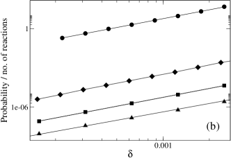
Figure 3: Collision probability (squares) and the number of reaction events (circles) as a function of the reaction distance $\delta$ for the blinking vortex-sink flow, with the same parameters as in Fig. 2. The initial conditions were chosen in the regions $R_{1}$ and $R_{2}$ defined in Fig. 2. The number of pairs used varied with $\delta$, and it was such that it guaranteed that at least $10^{3}$ collisions took place for each $\delta$; typically this meant the number of pairs was of order $10^{10}$–$10^{11}$. The straight lines are the fitting of the data to a power law of the form $\delta^{\beta^{*}}$; in both cases fitting yields $\beta^{*}=2.23$, compared to the prediction $\beta=2.25$ of Eq. (4). The collision probability for the area-preserving baker map with escape is also shown (diamonds), for contraction factors $0.3$ and $0.45$ Ott . Fitting yields $\beta^{*}=2.30$. For this system $D_{1}^{s}=1.701$ and $D_{2}^{u}=1.698$, and from Eq. (4) the prediction is $\beta=2.298$. The triangles show the collision probability for the conservative Hénon map for the nonlinearity parameter $\lambda=7$ Moura2004 , for which $D_{1}^{s}=1.58$ and $D_{2}^{u}=1.32$, leading to a prediction of $\beta=2.16$; fitting yields $\beta^{*}=2.14$. The baker map data (diamonds) in this plot has been shifted in the graph above to improve visibility.

Assuming that the particles advected by the flow behave as passive tracers, their equations of motion are PHR

$$\dot{r}=-C/r,\quad\dot{\varphi}=K/r^{2},$$ (5)

where $r$ and $\varphi$ are polar coordinates whose origin alternates between $(a,0)$, during the first half of each period, and $(-a,0)$, during the second half of each period; $C$ and $K$ are parameters representing the strengths of the sink and the vortex, respectively. The advection dynamics is determined by the two dimensionless parameters $\eta=CT/a^{2}$ and $\xi=K/C$, where $T$ is the flow period. We choose units so that $a=1$ and $T=1$. The dynamics is chaotic for a wide range of $\eta$ and $\xi$ PHR . Fig. 2a shows the unstable manifold for one particular choice of parameters, $\eta=0.5$ and $\xi=10$.

We computed the collision probability $p(\delta)$ by following the trajectories of many pairs of particles until one particle in each pair escapes, and at every time step $\Delta t$ we check if the distance between the two particles is less than $\delta$; if so, the particles are considered to have collided. The initial condition of one of the particles in each pair is chosen randomly within region $R_{1}$, defined in the caption of Fig. 2; and the other particle in the pair is started in region $R_{2}$ (see Fig. 2). The fraction of the pairs which collide before escaping gives us a numerical approximation of $p(\delta)$. Figure 3 (the squares) shows the result of applying this procedure for a range of values of $\delta$. The resulting scaling is clearly a power law $p(\delta)\sim\delta^{\beta^{*}}$, and fitting yields $\beta^{*}\approx 2.25$. To compare this with the prediction of Eq. (4), we use the value $D_{1}^{s}\approx 1.74$ from PHR ; to compute $D_{2}^{u}$ we first find an approximation $W_{u}^{\rm spr}$ of the unstable manifold using the sprinkler method cscatbook , and then we compute the scaling with $\epsilon$ of the total number of pairs of points on $W_{u}^{\rm spr}$ separated by a distance less than $\epsilon$; the coefficient of the resulting power law is $D_{2}^{u}$ Grassberger1983 . We found $D_{2}^{u}\approx 1.71$. This is a two-dimensional system, and so $N=2$ in Eq. (4). Equation (4) then predicts $\beta=2.23$, which agrees with the value $\beta^{*}=2.25$ from the simulation, to within numerical errors.

Fig. 2a is a snapshot of $W_{u}$ at the start of a period; the shape of $W_{u}$ changes periodically with time, with the same period as the flow. Figure 2b shows the positions of the collisions that take place at the beginning of each period: each dot in Fig. 2b is one such collision. Comparing Figs. 2a and 2b, it is clear that the collisions take place in a small neighbourhood of the unstable manifold $W_{u}$, confirming that the assumption made in the derivation of Eq. (4) is correct.

We have analysed other choices of the parameters $\eta$ and $\xi$ for which the flow is chaotic, and we always find that the prediction from Eq. (4) and the results from the simulations differ by less than 1% in all cases. We found that the choice of the time step $\Delta t$ does not affect the scaling of $p(\delta)$ with $\delta$ — although the value of $p$ for any given $\delta$ of course decreases with $\Delta t$, since with larger time steps it is more likely collisions will be missed by the simulation.

We have also studied the dynamics of collisions in other two-dimensional dynamical systems, including a variant of the conservative Hénon map which displays transient chaos Moura2004 , and a version of the baker’s map with escape Ott . In all cases, and for all parameter choices, we found excellent agreement between the numerical value of $\beta$ and the prediction of Eq. (4) (see Fig. 3).

We now examine a system of reacting particles advected by a chaotic open flow. Taking as an illustrative example the case of an acid-base-type reaction $A+B\rightarrow C$, consider particles of two species, which we will label simply species $A$ and $B$, such that when an $A$ particle comes within a distance $\delta$ of a particle of type $B$, a reaction occurs, resulting in a particle of type $C$, which is the product of the reaction. If we throw $N_{1}$ type-$A$ particles in a region $R_{1}$ of the flow, and $N_{2}$ type-$B$ particles in region $R_{2}$, then we expect that the total number $N_{p}$ of type-$C$ particles produced in the system is proportional to $N_{1}N_{2}p(\delta)$ — as long as $N_{1}$ and $N_{2}$ are not too large, and the low-density assumption holds. We therefore predict that the amount $N_{p}$ of product generated by the reaction scales with the reaction distance $\delta$ as $\delta^{\beta}$, with $\beta$ given by Eq. (4).

We put this prediction to the test in the blinking vortex-sink system, using an efficient algorithm for finding the neighbours within a distance $\delta$ Bentley1975 . The resulting scaling of $N_{p}$ with $\delta$ is shown in Fig. 3. We find a power-law scaling as expected, and fitting yields the coefficient $\beta^{*}=2.25$, which is again within 1% of the predicted value of $\beta=2.23$. We found the same agreement for other choices of parameters for the blinking vortex-sink system, and also for the other dynamical systems we investigated.

We note that, even though we used the reaction $A+B\rightarrow C$ as an example above, all kinds of reactions and active processes involving particles will be affected by the scaling (4), since all reactions require particles to come close together, and the probability of that happening is governed by the coefficient $\beta$ of Eq. (4). We propose that the collision probability $p$, and the way is scales with the collision distance $\delta$, is the natural quantity to characterise the efficiency of mixing of an open flow (an alternative definition is given in Gouillart2011measures ). Equation (4) shows that the mixing efficiency is determined by the fractal properties of the invariant sets associated with the chaotic saddle — namely its stable and unstable manifolds. The discussion above shows that the mixing efficiency in turn determines the efficiency of chemical reactions (or, in general, active processes) in open flows, which means that the “chemical efficiency” of a flow is also measured by the coefficient $\beta$ defined in Eq. (4).

References

- (1) G. K. Batchelor, An introduction to fluid dynamics (Cambridge University Press, Cambridge, 1967)
- (2) C. Jung, T. Tél, and E. Ziemniak, Chaos 3, 555 (1993)
- (3) T. Tél, A. de Moura, C. Grebogi, and G. Károlyi, Phys. Rep. 413, 91 (2005)
- (4) A. D. Stroock et al, Science 295, 647 (2002)
- (5) T.-Y. Koh and B. Legras, Chaos 12, 382 (2002)
- (6) A. B. Schelin et al, Phys. Rev. E 80, 016213 (2009)
- (7) G. K rolyi et al, Proc Natl Acad Sci U S A 97, 13661 (2000)
- (8) E. Gouillart, O. Dauchot, J.-L. Thiffeault, and S. Roux, Phys. Fluids 21, 023603 (2009)
- (9) E. Gouillart, O. Dauchot, and J. Thiffeault, Phys. Fluids 23, 3604 (2011), ISSN 0899-8213
- (10) Y.-C. Lai and T. Tél, Transient chaos (Springer-Verlag, New York, 2011)
- (11) G. Károlyi et al, Phys Rev E 59, 5468 (1999)
- (12) G. K rolyi, T. T l, A. P. S. de Moura, and C. Grebogi, Phys. Rev. Lett. 92, 174101 (2004)
- (13) A. E. Motter, Y.-C. Lai, and C. Grebogi, Phys. Rev. E 68, 056307 (2003)
- (14) A. P. S. de Moura and C. Grebogi, Phys. Rev. E 70, 036216 (2004)
- (15) A. P. S. de Moura and C. Grebogi, Phys. Rev. E 70, 026218 (2004)
- (16) G. Metcalfe and J. M. Ottino, Phys Rev Lett 72, 2875 (1994)
- (17) T. Nishikawa, Z. Toroczkai, and C. Grebogi, Phys Rev Lett 87, 038301 (2001)
- (18) J. H. E. Cartwright et al, “Nonlinear dynamics and chaos: advances and perspectives,” (Springer-Verlag, 2010) p. 51
- (19) J. H. E. Cartwright et al, Phys Rev Lett 93, 035502 (2004)
- (20) M. Wilkinson, B. Mehlig, and V. Bezuglyy, Phys Rev Lett 97, 048501 (2006)
- (21) R. D. Vilela, T. T l, A. P. S. de Moura, and C. Grebogi, Phys. Rev. E 75, 065203 (2007)
- (22) M. Smoluchowski, Physik. Zeit. 17, 557 (1916)
- (23) P. Grassberger and I. Procaccia, Phys. Rev. Lett. 50, 346 (1983)
- (24) G. Károlyi and T. Tél, Phys. Rep. 290, 125 (1997)
- (25) H. Aref et al, Physica D 37, 423 (1989)
- (26) H. Aref, J. Fluid Mech. 143, 1 (1984)
- (27) E. Ott, Chaos in dynamical systems (Cambridge University Press, Cambdridge, 1993)
- (28) J. L. Bentley, Communications of the ACM 18, 509 (1975)