Relativistic cosmology number densities
and the luminosity function

Abstract

Aims. This paper studies the connection between the relativistic number density of galaxies down the past light cone in a Friedmann-Lemaître-Robertson-Walker spacetime with non-vanishing cosmological constant and the galaxy luminosity function (LF) data. It extends the redshift range of previous results presented in Albani et al., where the galaxy distribution was studied out to $z=1$. Observational inhomogeneities were detected at this range. This research also searches for LF evolution in the context of the framework advanced by Ribeiro and Stoeger, further developing the theory linking relativistic cosmology theory and LF data.

Methods. Selection functions are obtained using the Schechter parameters and redshift parametrization of the galaxy luminosity functions obtained from an I-band selected dataset of the FORS Deep Field galaxy survey in the redshift range $0.5\leq z\leq 5.0$ for its blue bands and $0.75\leq z\leq 3.0$ for its red ones. Differential number counts, densities and other related observables are obtained, and then used with the calculated selection functions to study the empirical radial distribution of the galaxies in a fully relativistic framework.

Results. The redshift range of the dataset used in this work, which is up to five times larger than the one used in previous studies, shows an increased relevance of the relativistic effects of expansion when compared to the evolution of the LF at the higher redshifts. The results also agree with the preliminary ones presented in Albani et al., suggesting a power-law behavior of relativistic densities at high redshifts when they are defined in terms of the luminosity distance.

1 Introduction

The galaxy volume number density, that is, the number of galaxies enclosed in a given volume, is a very important quantity in cosmology. It gives information about the density of the mass-energy in the universe and its evolution, allowing us to test various observational features of cosmological models like, for instance, the observational inhomogeneities of the number counts data down our past light cone (Albani et al. 2007). This important quantity can be observationally determined by a careful analysis of data from galaxy redshift surveys, as has been done in a systematic way by several authors who derived the galaxy luminosity function (LF) $\phi$ from such surveys. The LF of galaxies is a number density per unit of luminosity (Peacock 1999). The LF stemming from the galaxy distribution in a given dataset is commonly fitted using the profile due to Schechter (1976),

$$\phi(l)=\phi^{\ast}\,l^{\alpha}\,e^{-l},$$ (1)

where $l\equiv L/L_{\scriptscriptstyle*}$, $L$ being the observed luminosity, $L_{\scriptscriptstyle*}$ the luminosity scale parameter, $\phi^{\ast}$ a normalization parameter and $\alpha$ the faint-end slope parameter. Various papers on the LF have used a variety of datasets in different wavelength regions: Lin et al. (1999), Fried et al. (2001), Blanton et al. (2003), Pozzetti et al. (2003), Bell et al. (2003), Norman et al. (2004), Wilmer et al. (2006), Ly et al. (2007), and Tzanavaris & Georgantopoulos (2008) obtained Schechter-type LF parameters for galaxies with redshift values out to $z\sim 1.5$. Poli et al. (2003), and Rudnick et al. (2003) did the same for galaxies with redshift values out to $z\sim 3$. More recently Bouwens et al. (2007), and Gabasch et al. (2008) obtained those parameters for galaxies with redshift values out to $z\sim 6$. It was found that the LF evolves with redshift in all galaxy redshift surveys.

Using the LF data to study observational features of cosmological models requires, however, some model linking relativistic cosmology number count theory with LF astronomical data and practice. One approach to this theoretical link was developed by Ribeiro and Stoeger (2003; hereafter RS03), who started from very general relativistic considerations and then specialized their theoretical results, applying them to the LF data provided by the CNOC2 redshift survey (Lin et al. 1999). This provides an example of how such a link is established, as well as facilitating various consistency tests between the data and the expected number count predictions from the assumed cosmological model. In a sequel Albani et al. (2007; hereafter A07) used the same CNOC2 dataset to actually obtain and analyze various types of observational relativistic densities, that is, the ones defined on the observer’s past light cone.

The aim of this work is to further study the observed number densities of galaxies down the observer’s past light cone. We want to focus on observational inhomogeneities of the number count data, analyzing these with differential density and integral density measures in order to separate out the effects of cosmic expansion from the effect of LF evolution. As has been discussed in detail in A07 and in Rangel Lemos & Ribeiro (2008), these measures are capable of revealing observational inhomogeneities even in spatially homogeneous cosmological models. This is because spatial homogeneity is defined on constant time hypersurfaces, and is therefore a built-in feature of Friedmann cosmologies, whereas observational homogeneity is defined by measures of mass-energy densities remaining unchanged along the past light cone. We also seek to investigate if there is significant evidence of power-law behavior in the observed galaxy distribution at high values of redshift, since A07 detected such a behavior out to $z\approx 1$. The importance of power-laws comes from the fact that they are indicative of self-organized criticality in dynamical systems. In other words, scale invariant phenomena such as power laws are emergent features of a distribution, this being a mechanism by which complexity arises in nature through simple local interactions.

The study presented here expands the results presented in RS03 and A07, since the model specific equations obtained in RS03 were applicable only to LF data whose parameters assumed the Einstein-de Sitter (EdS) cosmology. And although the study presented in A07 was not limited to the EdS model, it was limited to the CNOC2 survey, which only probed out to $z=0.75$ and extrapolated to $z=1$. In addition, although both papers made some important theoretical connections between the relativistic cosmology equations and the LF data for a specific cosmology, they omitted important steps. These can be summarized as follows. The equations and methodology used in A07 for dealing with non-zero cosmological constant models are generalized, fully presented and discussed in this paper. An appendix containing a detailed algorithm on how to obtain the key results is also included. The role of the completeness function $J$ connecting theory and observations, as advanced in RS03, is made explicit here, adding clarity to the results and presenting them in a more straightforward manner. Finally, a comparison of the geometrical versus evolutionary effects, the latter being empirically obtained from the LF, on the relativistic volume number densities is discussed, considering a broad spectral classification of late versus early type galaxies. So, this work further advances the treatment of both RS03 and A07 and presents a comprehensive and detailed discussion of how one can proceed in applying the very general, model independent, relativistic cosmology equations to specific cosmologies, thus linking any cosmological model to LF data. This is necessary if we want to use LF data to observationally test more general cosmological models (any more general models will be inhomogeneous and/or anisotropic), a task we intend to carry out in forthcoming papers. Table 1 summarizes the new contributions of this paper as compared with the results obtained in the previous ones.

In this paper we assume a Friedmann-Lemaître-Robertson-Walker (FLRW) cosmology with non-zero cosmological constant $\Lambda$ and derive model independent relativistic equations which enable us to solve numerically expressions which include LF data. The numerical scheme is presented in detail and applied to a galaxy redshift survey dataset that assumes the FLRW standard cosmological model in its volume and distance definitions: the I-band selected luminosity functions of Gabasch et al. (2004 and 2006; hereafter G04 and G06 respectively) for the FORS Deep Field (FDF). From the Schechter parameters and their redshift parametrization appearing in G04 and G06, we calculated the selection functions $\psi$ in eight bandwidths and in equally spaced redshift intervals of 0.25 spanning the range $0.5\leq z\leq 5.0$, for the blue bands (G04), and $0.75\leq z\leq 3.0$ for the red bands (G06). Once the selection functions were calculated, we were able to obtain the observational number counts, differential number counts and differential and integral densities, as defined in RS03 and Ribeiro (2005) and further discussed in A07 and Rangel Lemos & Ribeiro (2008). These quantities were then used to study observational inhomogeneities in the relativistic radial distribution of galaxies belonging to that dataset. Therefore, the calculations of this paper go to much higher redshift than the ones presented in A07. The results reached here generally agree with theirs, also indicating that observational inhomogeneities in the relativistic galaxy distributions can arise due to geometrical, null-geodesic effects, even in the context of spatially homogeneous universes (Ribeiro 1992, 1995, 2001, 2005; Rangel Lemos & Ribeiro 2008).

The plan of the paper is as follows. In §2 we briefly present the FLRW model, basically to set up notation and write essential results. Then we apply the general, model independent, equations of relativistic cosmology number-count theory to this universe model in order to obtain the differential equations governing the evolution of the two basic quantities of our analysis, namely, the scale factor and the relativistic number counts. §3 describes in detail our numerical approach for solving these two differential equations, as well as our procedures for deriving all other quantities relevant in our analysis. In doing that we also explain how they connect to the the scale factor and the number counts. In §4 we further develop general equations connecting LF data with relativistic cosmology number-count theory and obtain the selection functions for the FDF dataset. In §5 we study the behavior of radial statistics of the relativistic densities obtained in the context of the FLRW model with $\Lambda\not=0$ and out to $z=5.0$. We present our conclusions in §6. The appendix presents an algorithm detailing how the methodology discussed in §2, §3 and §4 can be applied to a given parametrized LF in order to obtain the observational relativistic densities discussed in §5.

2 Standard cosmology with non-zero cosmological constant

2.1 The scale factor

We begin by writing the FLRW line element as follows,

$$ds^{2}=-\;c^{2}dt^{2}+S^{2}\left[\frac{dr^{2}}{1-kr^{2}}+r^{2}\left(d\theta^{2}+\sin^{2}\theta\;d\phi^{2}\right)\right],$$ (2)

where the time-dependent function $S=S(t)$ is the cosmic scale factor, $k$ is the curvature parameter $(k=+1,0,-1)$ and $c$ is the light speed. As is well known, the Einstein’s field equations with the metric corresponding to this line element yields the Friedmann equation, which, if the cosmological constant $\Lambda$ is included, may be written (e.g. Roos 1994),

$$H^{2}=\frac{8\pi G\rho_{m}}{3}+\frac{\Lambda}{3}-\frac{kc^{2}}{S^{2}},$$ (3)

where $\rho_{m}$ is the matter density and we have assumed the usual definition for the Hubble parameter,

$$H(t)\equiv\frac{1}{S(t)}\frac{dS(t)}{dt}.$$ (4)

Let us now define the vacuum energy density in terms of the cosmological constant,

$$\rho_{\Lambda}\equiv\frac{\Lambda}{8\pi G}.$$ (5)

Since the critical density at the present time is given by,

$${\rho_{0,c}\equiv\frac{3{H_{0}}^{2}}{8\pi G}},$$ (6)

where $H_{0}$ is the Hubble constant, the following relative-to-critical density parameter relations hold,

$$\Omega_{0}\equiv\Omega_{m_{0}}+\Omega_{\Lambda_{0}}={\frac{\rho_{0}}{\rho_{0,c}}=\frac{\rho_{m_{0}}}{\rho_{0,c}}+\frac{\rho_{\Lambda_{0}}}{\rho_{0,c}}}.$$ (7)

We have used the zero index to indicate observable quantities at the present time. Notice that since $\Lambda$ is a constant, then $\rho_{\Lambda}=\rho_{\Lambda_{0}}$. Considering the definitions (7), we can rewrite the Friedmann equation (3) at the present time as follows,

$$kc^{2}={H_{0}}^{2}{S_{0}}^{2}(\Omega_{0}-1).$$ (8)

In addition, from the law of conservation of energy applied to the zero pressure, matter dominated era, we know that,

$$\rho_{m}\propto S^{-3}\;\;\Rightarrow\;\;\rho_{m_{0}}\propto{S_{0}}^{-3},$$ (9)

which leads to,

$$\frac{\rho_{m}}{\rho_{m_{0}}}=\frac{{S_{0}}^{3}}{S^{3}}\;\;\Rightarrow\;\;\Omega_{m}=\Omega_{m_{0}}\frac{{S_{0}}^{3}{H_{0}}^{2}}{S^{3}H^{2}},$$ (10)

since the matter-density parameter can also be written in terms of the critical density as,

$$\Omega_{m}=\frac{\rho_{m}}{\rho_{c}}=\frac{8\pi G}{3{H}^{2}}\,{\rho_{m}}.$$ (11)

We can rewrite equation (3) as a first order ordinary differential equation in terms of the scale factor $S(t)$, by using the results in equations (4)-(11), yielding,

$$\frac{dS}{dt}=H_{0}{\left[\frac{\Omega_{m_{0}}{S_{0}}^{3}}{S}+\Omega_{\Lambda_{0}}{S}^{2}-(\Omega_{0}-1){S_{0}}^{2}\right]}^{1/2}.$$ (12)

The problem we deal with in this paper requires the solution of the equation above as well as of another differential equation for the cumulative number count $N$ (see eq. 20 below). The simplest approach is to simultaneously solve these two differential equations by numerical means.

2.2 Relativistic number counts

Let us write the completely general, cosmological, model-independent expression derived by Ellis (1971) for the number count of cosmological sources, which takes fully into account relativistic effects, as follows,

$$dN=(d_{\scriptscriptstyle A})^{2}d\Omega[n(-k^{a}u_{a})]_{P}\;dy.$$ (13)

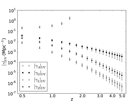
Figure 1: Observational relativistic differential densities versus redshift in the combined UV bands of the FDF dataset of G04. Symbols are as in the legend.

Here $dN$ is the number of cosmological sources in a volume section at a point P down the null cone, $n$ is the number density of radiating sources per unit of proper volume in a section of a bundle of light rays converging towards the observer and subtending a solid angle $d\Omega$ at the observer’s position, $d_{\scriptscriptstyle A}$ is the area distance of this section from the observer’s viewpoint (also known as angular diameter distance, observer area distance and corrected luminosity distance), $u^{a}$ is the observer’s 4-velocity, $k^{a}$ is the tangent vector along the light rays and $y$ is the affine parameter distance down the light cone constituting the bundle (see RS03, §2.1, figure 1). The number density, that is, the number of cosmological sources per proper volume unit, can be related to the matter density $\rho_{m}$ by means of,

$$n=\frac{\rho_{m}}{{\cal M}_{g}}.$$ (14)

where, ${\cal M}_{g}$ is simply the average galaxy rest mass, dark matter included.

One should point out that the details of the galaxy mass function and how it evolves with the redshift are imprinted in the LF itself. As a consequence, it will be included in any selection functions stemming from the LF. For the empirical purposes of this paper this equation is correct to an order of magnitude and should be regarded only as an estimate. This means that equation (14) enables us to connect the theoretical relativistic quantities to the LF data and thus include the redshift evolution of the mass function empirically (more on this point at the end of §4.1 below). However, to actually extract from the LF its implicit galaxy mass function requires some assumption about the function ${\cal M}_{g}(z)$. We shall deal with this problem in a forthcoming paper.

So, for the empirical approach of this paper it is enough to assume a constant average galaxy rest mass with the working value of ${\cal M}_{g}\approx 10^{11}{M}_{\sun}$ based on the estimate by Sparke & Gallagher (2000). Hence, if we use equations (10) and (11) we can rewrite equation (14) as,

$$n=\left(\frac{3\Omega_{m_{0}}{H_{0}}^{2}{S_{0}}^{3}}{8\pi G{\cal M}_{g}}\right)\frac{1}{S^{3}}.$$ (15)

The past radial null geodesic in the geometry given by metric (2) may be written

$$\frac{dt}{dr}=-\left(\frac{S}{c\sqrt{1-kr^{2}}}\right).$$ (16)

Since both coordinates $t$ and $r$ are functions of the affine parameter $y$ along the past null cone, we have that

$$\frac{dt}{dy}=\frac{dt}{dr}\frac{dr}{dy}=-\left(\frac{S}{c\sqrt{1-kr^{2}}}\right)\frac{dr}{dy}.$$ (17)

Assuming now that both source and observer are comoving, then $u^{a}=c\;{\delta_{0}}^{a}$ and the following results hold,

$$-k^{a}u_{a}=-c\;k^{a}g_{0a}=-c\;k^{0}=-c\frac{dt}{dy}=\left(\frac{S}{\sqrt{1-kr^{2}}}\right)\frac{dr}{dy}.$$ (18)

In addition, remembering that the area distance $d_{\scriptscriptstyle A}$ is defined by means of a relation between the intrinsically measured cross-sectional area element $d\sigma$ of the source and the observed solid angle $d\Omega_{0}$ (Ellis 1971, 2007; Plebański & Krasiński 2006), we have that

$$(d_{\scriptscriptstyle A})^{2}=\frac{d\sigma}{d\Omega}=\frac{S^{2}r^{2}(d\theta^{2}+\sin^{2}\theta\;d\phi^{2})}{(d\theta^{2}+\sin^{2}\theta\;d\phi^{2})}=(Sr)^{2}.$$ (19)

We note that for this metric the area distance, a strictly observational distance definition, equals the proper distance $d_{\scriptscriptstyle Pr}$, a relativistic one. Considering equation (8) and substituting equations (15), (18) and (19) into equation (13), and remembering that here $d\Omega_{0}=4\pi$, we are then able to write the number of sources along the past light cone in terms of the radial coordinate $r$ and in the FLRW model defined in §2.1. This quantity is given by the following expression,

$$\frac{dN}{dr}=\left(\frac{3\;c\;\Omega_{m_{0}}{H_{0}}^{2}{S_{0}}^{3}}{2G{\cal M}_{g}}\right)\left[\frac{r^{2}}{\sqrt{c^{2}-{H_{0}}^{2}{S_{0}}^{2}(\Omega_{0}-1)r^{2}}}\right].$$ (20)

3 Numerical problem

The differential equations for the scale factor $S$ and the cumulative number count $N$, equations (12) and (20) respectively, provide the basic quantities necessary here, since the expressions which actually connect the relativistic theory to LF data are built upon them. However, before these two differential equations can be solved numerically, some further algebraic manipulations are necessary. Next we shall describe these steps and how other quantities relevant to our analysis are written in terms of these two functions.

The numerical problem can be summarized as follows. We take the radial coordinate $r$ as the independent variable in order to numerically obtain the functions $N(r)$ and $S(r)$ along the past light cone. Then all other quantities of interest are written in terms of these two functions, meaning that numerical results for $N(r)$ and $S(r)$ allow us to straightforwardly obtain $z\>(r)$ and $dN/dz\>(r)$, as well as various cosmological distances, their derivatives, observational volumes and number densities. Thus, all quantities used in our analysis end up being written in terms of the radial coordinate $r$.

3.1 Scale factor

A simple and straightforward approach to solving the differential equations for the scale factor $S$ and the cumulative number count $N$ is to take the radial coordinate $r$ as the independent variable and simultaneously integrate them by numerical means. To do so we shall proceed as follows.

Equation (12) has its time coordinate implicitly defined in the scale factor, therefore we need to rewrite that differential equation in such a way that the independent variable becomes explicit. Considering equation (8), the null geodesic (16) becomes,

$$\frac{dt}{dr}=-\left[\frac{S^{2}}{c^{2}-{H_{0}}^{2}{S_{0}}^{2}(\Omega_{0}-1)r^{2}}\right]^{\frac{1}{2}}.$$ (21)

Along the past light cone, we can write the scale factor in terms of the radial coordinate as

$$\frac{dS}{dr}=\frac{dS}{dt}\frac{dt}{dr}.$$ (22)

Thus, we are able to rewrite equation (12) in terms of the radial coordinate,

$$\frac{dS}{dr}=-H_{0}\left[\frac{(\Omega_{\Lambda_{0}})S^{4}-{S_{0}}^{2}(\Omega_{0}-1)S^{2}+(\Omega_{m_{0}}{S_{0}}^{3})S}{c^{2}-{H_{0}}^{2}{S_{0}}^{2}(\Omega_{0}-1)r^{2}}\right]^{\frac{1}{2}}.$$ (23)

To find solutions for $S(r)$ we must assume numerical values for $\Omega_{m_{0}}$, $\Omega_{\Lambda_{0}}$ and $H_{0}$. In this paper we adopt the FLRW model with $\Omega_{m_{\scriptscriptstyle 0}}=0.3$, $\Omega_{\Lambda_{\scriptscriptstyle 0}}=0.7$ and $H_{0}=70\;\mbox{km}\;{\mbox{s}}^{-1}\;{\mbox{Mpc}}^{-1}$.

The two differential equations (20) and (23) comprise our numerical problem. Solving them simultaneously enables us to generate tables for $r$, $S$ and $N$. A computer code using the fourth-order Runge-Kutta method is good enough to successfully carry out the numerical tasks. The initial conditions $r_{0}$ and $N_{0}$ are set to zero, whereas $S_{0}$ can be derived considering that as $r\rightarrow 0$ the spacetime is approximately Euclidean, that is, $k\approx 0$. This leads, from equation (16), to ${ct=-r}$ as well as $S_{0}=1$.

3.2 Differential number count

The redshift $z$ can be written as

$$1+z=\frac{S_{0}}{S},$$ (24)

where it is clear that a numerical solution of the scale factor $S(r)$ immediately gives us the numerical solution for $z(r)$. We can derive the differential number counts $dN/dz$ by means of the expression,

$$\frac{dN}{dz}=\frac{dr}{dz}\frac{dN}{dr},$$ (25)

with the help of the useful relation

$$\frac{dr}{dz}=\frac{dr}{dS}\frac{dS}{dz}.$$ (26)

Numerically, since we build all our quantities using $N(r)$ and $S(r)$, any derivative with respect to the redshift we wish to evaluate will be similarly written in terms of the derivative of that quantity in terms of the radial coordinate. The derivatives in equation (26) can be taken from definition (24) and equation (23), enabling us to write,

$$\frac{dr}{dz}=\frac{S^{2}}{S_{\scriptscriptstyle 0}\,H_{\scriptscriptstyle 0}}\left[\frac{(\Omega_{\Lambda_{0}})S^{4}-{S_{0}}^{2}(\Omega_{0}-1)S^{2}+(\Omega_{m_{0}}{S_{0}}^{3})S}{c^{2}-{H_{0}}^{2}{S_{0}}^{2}(\Omega_{0}-1)r^{2}}\right]^{-\frac{1}{2}}.$$ (27)

This, together with equation (20), allows us to write equation (25) as,

$$\frac{dN}{dz} = \left(\frac{3\;c\;\Omega_{m_{0}}H_{0}{S_{0}}^{2}}{2G{\cal M}_{g}}\right)\times$$ (28)

$$\times\left[\frac{r^{2}S^{2}}{\sqrt{(\Omega_{\Lambda_{0}})S^{4}-{S_{0}}^{2}(\Omega_{0}-1)S^{2}+(\Omega_{m_{0}}{S_{0}}^{3})S}}\right].$$

3.3 Proper and comoving volumes

As discussed in RS03, most cosmological densities obtained from astronomical observations assume comoving volumes, whereas densities derived from theory often assume the local, or proper, volumes. The luminosity function, for instance, is nowadays always obtained from galaxy catalogues by assuming the comoving volume in its calculation. So, we are only able to compare those observationally derived parameters with theory if we carry out a conversion of volume units. From metric (2) it is obvious that,

$$dV_{\scriptscriptstyle Pr}=\frac{S^{3}}{\sqrt{1-kr^{2}}}r^{2}dr\sin\theta d\theta d\phi=S^{3}dV_{\scriptscriptstyle C},$$ (29)

This equation clearly defines the conversion factor between these two volume definitions.

3.4 Distance measures

So far we have used only the area distance $d_{\scriptscriptstyle A}$ as distance definition. However, other cosmological distances can, and will, be used later. They can be easily obtained from the area distance by invoking Etherington’s reciprocity law (Etherington 1933; Ellis 1971, 2007),

$$d_{\scriptscriptstyle L}=(1+z)^{2}d_{\scriptscriptstyle A}=(1+z)\;d_{\scriptscriptstyle G}.$$ (30)

Here $d_{\scriptscriptstyle L}$ is the luminosity distance and $d_{\scriptscriptstyle G}$ is the galaxy-area distance. The latter is also known as angular-diameter distance, transverse comoving distance or proper-motion distance. A fourth distance will also be useful later, the redshift distance $d_{z}$, defined by the following equation,

$$d_{z}=\frac{c\>z}{H_{0}}.$$ (31)

Although the reciprocity law is independent of any cosmological model, the detailed calculations presented in the previous sections are for the FLRW cosmology only. This means that in deriving $d_{\scriptscriptstyle A}$, $d_{\scriptscriptstyle L}$, $d_{\scriptscriptstyle G}$ and $d_{z}$ we write the FLRW expression for $d_{\scriptscriptstyle A}$ and derive the others using the general, model independent, expression (30), as well as equation (31). Thus, considering equation (19) for $d_{\scriptscriptstyle A}$ and the reciprocity theorem (30), it is straightforward to write the other cosmological distances in terms of the scale factor, as follows,

$$d_{\scriptscriptstyle L}={S_{0}}^{2}\left(\frac{r}{S}\right),$$ (32)

$$d_{\scriptscriptstyle G}=S_{0}\>r,$$ (33)

$$d_{z}=\frac{c}{H_{0}}\left(\frac{S_{0}}{S}-1\right).$$ (34)

The derivatives of each distance with respect to the redshift still need to be determined since they will be necessary later. Starting with the area distance $d_{\scriptscriptstyle A}$, they can be easily obtained from equations (19) and (24). Then it follows that,

$$\frac{d(d_{\scriptscriptstyle A})}{dz}=\frac{dS}{dz}\frac{dr}{dS}\frac{d(d_{\scriptscriptstyle A})}{dr}=-\frac{S^{2}}{S_{0}}\left[r+S{\left(\frac{dS}{dr}\right)}^{-1}\right].$$ (35)

Using equation (23), this expression may be rewritten as,

$$\frac{d(d_{\scriptscriptstyle A})}{dz} = \frac{S^{2}}{S_{0}}\left[\frac{S}{H_{0}}\sqrt{\frac{{c^{2}-{H_{0}}^{2}{S_{0}}^{2}(\Omega_{0}-1)r^{2}}}{{(\Omega_{\Lambda_{0}})S^{4}-{S_{0}}^{2}(\Omega_{0}-1)S^{2}+(\Omega_{m_{0}}{S_{0}}^{3})S}}}\right.\;-$$ (36)

$$\biggl{.}-\;r\biggr{]}.$$

The other observational distances can be numerically calculated from equation (35) if we consider the reciprocity law (30). Therefore, we have,

$$\frac{d(d_{\scriptscriptstyle L})}{dz}=2(1+z)d_{\scriptscriptstyle A}+(1+z)^{2}\frac{d(d_{\scriptscriptstyle A})}{dz},$$ (37)

$$\frac{d(d_{\scriptscriptstyle G})}{dz}=d_{\scriptscriptstyle A}+(1+z)\frac{d(d_{\scriptscriptstyle A})}{dz}.$$ (38)

These two equations can also be rewritten in terms of the scale factor if we consider equations (24) and (36), yielding,

$$\frac{d(d_{\scriptscriptstyle L})}{dz} = S_{0}\left[\frac{S}{H_{0}}\sqrt{\frac{{c^{2}-{H_{0}}^{2}{S_{0}}^{2}(\Omega_{0}-1)r^{2}}}{{(\Omega_{\Lambda_{0}})S^{4}-{S_{0}}^{2}(\Omega_{0}-1)S^{2}+(\Omega_{m_{0}}{S_{0}}^{3})S}}}\;+\right.$$ (39)

$$+\;\biggl{.}r\biggr{]},$$

$$\frac{d(d_{\scriptscriptstyle G})}{dz}=\frac{S^{2}}{H_{0}}\sqrt{\frac{{c^{2}-{H_{0}}^{2}{S_{0}}^{2}(\Omega_{0}-1)r^{2}}}{{(\Omega_{\Lambda_{0}})S^{4}-{S_{0}}^{2}(\Omega_{0}-1)S^{2}+(\Omega_{m_{0}}{S_{0}}^{3})S}}}\;.$$ (40)

From now on we shall generically use $d_{\scriptscriptstyle i}$ to indicate any observational distance, which can be any one of the four cosmological distances defined above ($i={\scriptstyle A}$, ${\scriptstyle G}$, ${\scriptstyle L}$, ${\scriptstyle Z}$).

3.5 Differential and integral densities

The differential density $\gamma_{\scriptscriptstyle i}$ gives the rate of growth in number counts, or more exactly in their density, as one moves along the observational distance $d_{\scriptscriptstyle i}$. It is defined by (Ribeiro 2005; Albani et al. 2007; Rangel Lemos & Ribeiro 2008),

$$\gamma_{\scriptscriptstyle i}=\frac{1}{4\pi(d_{\scriptscriptstyle i})^{2}}\frac{dN}{d(d_{\scriptscriptstyle i})},$$ (41)

whereas the integrated differential density, or simply integral density, gives the number of sources per unit of observational volume located inside the observer’s past light cone out to a distance $d_{\scriptscriptstyle i}$. Is is written as,

$$\gamma_{\scriptscriptstyle i}^{\ast}=\frac{1}{V_{\scriptscriptstyle i}}\int\limits_{V_{\scriptscriptstyle i}}\gamma_{\scriptscriptstyle i}\;dV_{\scriptscriptstyle i},$$ (42)

where $V_{\scriptscriptstyle i}$ is the observational volume,

$$V_{\scriptscriptstyle i}=\frac{4}{3}\pi(d_{\scriptscriptstyle i})^{3}.$$ (43)

These quantities are useful in determining whether or not, and within what ranges, a spatially homogeneous cosmological model can or cannot be observationally homogeneous as well (Ribeiro 1995, 2005; Rangel Lemos & Ribeiro 2008). This is because these densities behave very differently depending on the distance measure used in their definitions – that is, they show a strong dependence on the cosmological distance adopted. Therefore, as discussed in Rangel Lemos & Ribeiro (2008), these measures are the ones we employ in this paper, because they are capable of probing the possible observational inhomogeneity of the number counts.

From a numerical viewpoint it is preferable to write the densities given by equations (41) and (42) in terms of the redshift. Thus, the differential density (41) may be written as,

$$\gamma_{\scriptscriptstyle i}=\frac{dN}{dz}\left\{4\pi(d_{\scriptscriptstyle i})^{2}\;\frac{d(d_{\scriptscriptstyle i})}{dz}\right\}^{-1}.$$ (44)

A final point still needs to be discussed. The integral density (42) is a result of integrating $\gamma_{\scriptscriptstyle i}$ over an observational volume. The simplest way of numerically deriving it is shown in what follows. Let us differentiate $\gamma_{\scriptscriptstyle i}^{\ast}$ in terms of the volume, so that,

$$\frac{d\left(\gamma_{\scriptscriptstyle i}^{\ast}V_{\scriptscriptstyle i}\right)}{dV_{\scriptscriptstyle i}}=\gamma_{\scriptscriptstyle i}.$$ (45)

Considering equation (44), this result leads to the following expression,

$$\frac{d\left(\gamma_{\scriptscriptstyle i}^{\ast}V_{\scriptscriptstyle i}\right)}{dz}=\frac{d\left(\gamma_{\scriptscriptstyle i}^{\ast}V_{\scriptscriptstyle i}\right)}{dV_{i}}\frac{dV_{i}}{dz}=\gamma_{\scriptscriptstyle i}\frac{dV_{i}}{dz}=\frac{dN}{dz}.$$ (46)

Similarly, it is simple to show that,

$$\frac{d\left(\gamma_{\scriptscriptstyle i}^{\ast}V_{\scriptscriptstyle i}\right)}{dr}=\frac{dN}{dr}.$$ (47)

Finally, from these two equations above, as well as from the definitions of $\gamma_{\scriptscriptstyle i}$ and $\gamma_{\scriptscriptstyle i}^{\ast}$, it is easy to conclude that the following expression holds,

$$\gamma_{\scriptscriptstyle i}^{\ast}=\frac{N}{V_{\scriptscriptstyle i}}.$$ (48)

So, the numerical solution of equation (20) together with the numerical determination of all distances, as given by equations (19), (32), (33), (34), allow us to calculate the volume (43) and evaluate $\gamma_{\scriptscriptstyle i}^{\ast}$. These results fully determine the numerical problem for the cosmological model under study.

In conclusion, once $N(r)$ and $S(r)$ are calculated along the past light cone in terms of the radial coordinate $r$, all other quantities are straightforwardly obtained with the same functional dependence: $z\>(r)$, $dN/dz\>(r)$, $d_{i}\,(r)$, $d(d_{i})/dz\>(r)$, $\gamma_{i}\>(r)$, $V_{i}\>(r)$ and $\gamma^{\ast}_{i}\>(r)$.

4 Observational quantities

We shall now specialize the equations above to obtain their observational counterparts based on the LF data from a specific galaxy catalog. As a direct consequence, we show how these results can be used to test the consistency of the number count theory detailed above.

4.1 General equations

Generally speaking, we shall assume that an observational quantity $[T]_{{\textstyle{\scriptscriptstyle obs}}}$ can be related to its theoretical counterpart $T$ by means of a completeness function $J$, such that,

$$[T]_{{\textstyle{\scriptscriptstyle obs}}}=J\,T.$$ (49)

RS03 showed that such a completeness function can be obtained by relating the selection function $\psi$, which gives the number of galaxies with luminosity above a given threshold in a given comoving volume, to the radial number density $n_{\scriptscriptstyle C}\,(z)$ in comoving volume units – that is, the number of sources in a given comoving volume. As already mentioned, it is common practice to adopt this volume definition to calculate the LF from galaxy datasets. The volume number density $n$ obtained in equation (15) comes from the right hand side of Einstein’s field equations and, therefore, it is written in terms of the proper volume. Thus, equation (15) must have its volume units corrected by means of equation (29) in order for the former to be correctly related to a selection function $\psi$ stemming from the LF.

The relationship allowing us to calculate the completeness function used in this work may be written,

$$\psi(z)=J(z)\,n_{\scriptscriptstyle C}(z).$$ (50)

Now, if we go back to equation (14) and the discussion in the paragraph below it, we can see that applying the completeness function by means of equation (49) actually means replacing the theoretical comoving number density $n_{\scriptscriptstyle C}$, based on a constant average galaxy rest mass, with its observed counterpart $\psi$ obtained directly from the LF. In that sense, all the observational quantities obtained by applying $J(z)$ to their theoretical counterparts will inherit that same empirical number count redshift evolution encoded in the parametrization of the LF. As the goal of this paper is to consider the effect of redshift evolution on the relativistic number densities, such an approach should suffice. Also, in equation (50) the completeness function is independent of volume units, therefore, if an observational quantity is obtained using $J(z)$ by means of equation (49) its original volume units dependence is preserved.

The selection function may be written in terms of the LF,

$$\psi(z)=\int^{\infty}_{l(z)}\phi(l)dl,$$ (51)

where $l(z)$ is the lower luminosity threshold below which the sources are not observed. The theoretical radial number density in comoving volume is given by,

$$n_{\scriptscriptstyle C}=\frac{N}{V_{\scriptscriptstyle C}}=\frac{3\,N(r)}{4\,\pi\,r^{3}}.$$ (52)

Most observational quantities of interest studied in this paper require previous knowledge of the observed differential number counts $[dN]_{{\textstyle{\scriptscriptstyle obs}}}$. Therefore, linking this quantity to its theoretical counterpart is an essential step in order to apply Ellis’ equation (13). In view of this, to find $[dN]_{{\textstyle{\scriptscriptstyle obs}}}$ we identify $T$ as $dN$ in equation (49), yielding,

$$\left[dN\right]_{{\textstyle{\scriptscriptstyle obs}}}=J(z){dN}.$$ (53)

In essence this expression describes the same number counts as in equation (50) and both are in agreement with Ellis’ (1971) key equation (13). Considering now both equations (50) and (53), it easily follows that,

$$\left[\frac{dN}{dz}\right]_{{\textstyle{\scriptscriptstyle obs}}}=J(z)\frac{dN}{dz}=\frac{\psi(z)}{n_{\scriptscriptstyle C}(z)}\frac{dN}{dz}.$$ (54)

This is our key equation relating the relativistic theory to the observations. The number density of a proper volume is given by

$$n=\frac{N}{V_{\scriptscriptstyle Pr}},$$ (55)

whereas the number density of a comoving volume is given by equation (52). Thus, we may rewrite equation (54) as follows,

$$\left[\frac{dN}{dz}\right]_{{\textstyle{\scriptscriptstyle obs}}}=\frac{V_{\scriptscriptstyle C}}{V_{\scriptscriptstyle Pr}}\frac{\psi}{n}\frac{dN}{dz}.$$ (56)

It is important to point out that the volume transformation in this equation merely reflects the fact that $J(z)$ is independent of volume units, proper or comoving, and does not in itself change the volume units underlying both $\left[dN/dz\right]_{{\textstyle{\scriptscriptstyle obs}}}$ and $dN/dz$ when they are derived by means of Ellis’ equation (13). It is the number density $n$ in equation (13) that defines the volume units of both $\left[dN/dz\right]_{{\textstyle{\scriptscriptstyle obs}}}$ and $dN/dz$ (see below).

A further step towards writing these results in terms of the underlying cosmology is taken if we remember that RS03 showed that Ellis’ (1971) differential number counts (13) can be rewritten

$$\frac{dN}{dz}=n\,(d_{\scriptscriptstyle A})^{2}\,(1+z)\,d\Omega\,\frac{dy}{dz}.$$ (57)

Thus, equation (56) becomes

$$\left[\frac{dN}{dz}\right]_{{\textstyle{\scriptscriptstyle obs}}}=\left[\frac{V_{\scriptscriptstyle C}}{V_{\scriptscriptstyle Pr}}(d_{\scriptscriptstyle A})^{2}\,(1+z)\,d\Omega\;\frac{dy}{dz}\right]\psi.$$ (58)

Note that in this expression $\left[dN/dz\right]_{{\textstyle{\scriptscriptstyle obs}}}$ is given in terms of proper volume units because the number density $n$ is written in terms of proper volume units. Also note that these expressions are general and independent of any cosmological model. The specific cosmology will appear once we specialize the terms inside the brackets on the right hand side.

Galaxy redshift surveys use bandwidth filters, and they sometimes include some sort of morphological classification. Therefore, a selection function $\psi$ which considers a set of filters $W$, and morphological types $v$, may be written as follows (see A07, eqs. 3-10),

$$\psi(z)=\sum_{\scriptscriptstyle W}a_{\scriptscriptstyle W}\frac{\sum_{\scriptscriptstyle v}P_{\scriptscriptstyle v}\,{\cal M}_{\scriptscriptstyle v}\>\psi^{\scriptscriptstyle W}_{\scriptscriptstyle v}(z)}{\sum_{\scriptscriptstyle v}P_{\scriptscriptstyle v}\,{\cal M}_{\scriptscriptstyle v}}.$$ (59)

Here $P_{\scriptscriptstyle v}$ is the fraction of galaxies in the dataset that were classified with the morphological type $v$ (see RS03, eq. 13), ${\cal M}_{\scriptscriptstyle v}$ is the typical local rest-mass value for a galaxy of the morphological type $v$, and $a_{\scriptscriptstyle W}$ are constants introduced to avoid multiple counting of the same objects in the various filters, defined as follows (see RS03, eq. 46),

$$a_{\scriptscriptstyle W}(z)=1,\;\;\;\;\mbox{for}\;\;\;\;W=1,$$ (60)

and

$$a_{\scriptscriptstyle W}(z)<1,\;\;\;\;\mbox{for}\;\;\;\;W>1.$$ (61)

Equation (61) simply states that when there exists more than one observed waveband ($W>1$), $a_{\scriptscriptstyle W}$ gives the fraction of galaxies in waveband $W>1$ that are not counted in wavebands $1,2,\ldots,(W-1)$. Considering these expressions, the completeness function defined in equation (50) can be rewritten

$$J(z)=\frac{1}{n_{\scriptscriptstyle C}(z)}\sum_{\scriptscriptstyle W}a_{\scriptscriptstyle W}\frac{\sum_{\scriptscriptstyle v}P_{\scriptscriptstyle v}\,{\cal M}_{\scriptscriptstyle v}\psi^{\scriptscriptstyle W}_{\scriptscriptstyle v}(z)}{\sum_{\scriptscriptstyle v}P_{\scriptscriptstyle v}\,{\cal M}_{\scriptscriptstyle v}}.$$ (62)

Substituting the expression (59) in equation (58) we obtain the following result,

$$\left[\frac{dN}{dz}\right]_{{\textstyle{\scriptscriptstyle obs}}}=\left[\frac{V_{\scriptscriptstyle C}}{V_{\scriptscriptstyle Pr}}(d_{\scriptscriptstyle A})^{2}(1+z)d\Omega\frac{dy}{dz}\right]\sum_{\scriptscriptstyle W}a_{\scriptscriptstyle W}\frac{\sum_{\scriptscriptstyle v}P_{\scriptscriptstyle v}{\cal M}_{\scriptscriptstyle v}\psi^{\scriptscriptstyle W}_{\scriptscriptstyle v}}{\sum_{\scriptscriptstyle v}P_{\scriptscriptstyle v}{\cal M}_{\scriptscriptstyle v}}.$$ (63)

This expression already appeared in A07. Here it has been reached through a more straightforward and simpler derivation and with the volume dependence explicitly shown. This means that volume conversions like the one discussed above in §3.3 may be needed if we are to calculate the observational differential number count $[dN/dz]_{{\textstyle{\scriptscriptstyle obs}}}$ in a consistent way. The above equation is shown here only to make explicit how the methodology of previous work can be understood in relationship to that being developed in this paper. In addition, it is important to note that equations (54), (56) and (63) are closely related. The first two are written in a more compact form, whereas the last one expands the morphological and bandwidth dependencies of the selection function and the relativistic features of the underlying four-dimensional spacetime, as indicated by the expression (57).

Equation (63) also allows us to see how a theoretical mass evolution does not affect the differential number counts constructed with LF parameters. This is based on the form of the summation over $\scriptstyle W$, inasmuch as if we allow an evolution of the galactic mass by considering it dependent on the redshift, such a dependency will appear both in the numerator and the denominator of the summation and, therefore, cancels out, at least to first order. However, although mass evolution does not directly alter equation (63), it will indirectly change $[dN/dz]_{{\textstyle{\scriptscriptstyle obs}}}$ as the LF parameters used in its construction will include some form of source evolution. See §2.2 of A07 for more details.

4.2 Selection functions

To calculate the completeness function and, as a consequence, other observational quantities, we need to compute the selection functions with respect to redshift in a given galaxy survey. G04 and G06 fitted the LF Schechter parameters over the redshifts of 5558 I-band selected galaxies in the FORS Deep Field dataset, photometrically measured down to an apparent magnitude limit of $I_{\scriptscriptstyle AB}=26.8$. G04 and G06 also showed that the selection in the I-band is expected to miss less than 10% of the objects detected in the K-band, given that the AB-magnitudes of the I-band are half a magnitude deeper than those of the K-band, out to redshift 6, beyond which no signal is detectable in the I-band due to the Lyman break. Heidt et al. (2001) also argue that the I-band selection minimizes biases like dust absorption. All galaxies in those studies were therefore selected in the I-band and then had their magnitudes for each of the five blue bands (1500 Å, 2800 Å, $u^{\prime}$, $g^{\prime}$ and $B$) and the three red ones ($r^{\prime}$, $i^{\prime}$ and $z^{\prime}$) computed using the best fitting SED given by their authors’ photometric redshift code convolved with the associated filter function. Gabash et al. (2004, 2006) determined the photometric redshifts by fitting template spectra to the measured fluxes on the optical and near infrared images of the galaxies. Heidt et al. (2001) reported that approximately 80% of the objects in that sample were classified as Im/Irr-type, 15% as E/S0-type or Sa/Sb/Sc-type, and finally 5% as stars.

The redshift ranges of $0.75\leq z\leq 3.0$ for the red bands and $0.5\leq z\leq 5.0$ for the blue bands are large enough for checking possible observational inhomogeneities, since Rangel Lemos & Ribeiro (2008) showed that in the Einstein-de Sitter cosmology it is only theoretically possible, i.e., not observationally, to distinguish these two features when $z\gtrsim 0.1$, whereas for $z>0.5$ such a distinction becomes significant. Therefore, using galaxies whose measured redshifts are mostly greater than $z=1$ allows us to obtain data along the past light cone far enough from our present time hypersurface. One must remember that spatial homogeneity is defined on our constant time hypersurface whereas observational homogeneity occurs along our past light cone (Rangel Lemos & Ribeiro 2008; see also Ribeiro 1992, 1995, 2001, 2005).

To calculate the actual values of these functions, we begin by writing the result obtained in RS03 for the limited bandwidth version of the selection function of a given LF, fitted by a Schechter analytical profile, in terms of absolute magnitudes,

$$\psi^{\scriptscriptstyle W}(z)=0.4\ln 10\,\int_{-\infty}^{M^{\scriptscriptstyle W}_{\scriptscriptstyle lim}(z)}\phi^{\ast}(z)10^{0.4[1+\alpha(z)][M^{\ast}(z)-\bar{M}^{\scriptscriptstyle W}]}\times$$

$$\times\exp\{-10^{0.4[M^{\ast}(z)-\bar{M}_{\scriptscriptstyle W}]}\}d\bar{M}^{\scriptscriptstyle W},$$ (64)

where, as discussed earlier, the index $W$ indicates the bandwidth filter. The equations for the redshift evolution of the LF parameters adopted by G04 and G06 are,

$$\phi^{\ast}(z)=\phi^{\ast}_{\scriptscriptstyle 0}\,(1+z)^{B^{\scriptscriptstyle W}},$$

$$M^{\ast}(z)=M^{\ast}_{0}+A^{\scriptscriptstyle W}\ln(1+z),$$

$$\alpha(z)=\alpha_{\scriptscriptstyle 0},$$

with $A^{\scriptscriptstyle W}$ and $B^{\scriptscriptstyle W}$ being the evolution parameters fitted for the different $W$ bands and $M^{\ast}_{\scriptscriptstyle 0}$, $\phi^{\ast}_{\scriptscriptstyle 0}$ and $\alpha_{\scriptscriptstyle 0}$ the local (z $\approx$ 0) values of the Schechter parameters as defined in G04 and G06. Since all galaxies were detected and selected in the I-band, we can write,

$$M^{\scriptscriptstyle W}_{\scriptscriptstyle lim}(z)=M^{\scriptscriptstyle I}_{\scriptscriptstyle lim}(z)=I_{\scriptscriptstyle lim}-5\log[d_{\scriptscriptstyle L}(z)]-25+A^{\scriptscriptstyle I},$$ (65)

for a luminosity distance $d_{\scriptscriptstyle L}$ given in Mpc. $I_{\scriptscriptstyle lim}$ is the limiting apparent magnitude of the I-band of the FDF survey and equals to 26.8. Its reddening correction is $A^{\scriptscriptstyle I}=0.035$ (in Heidt et al. 2001). We computed the selection functions for all eight bands of the dataset by means of simple numerical integrations at equally spaced values spanning the whole redshift interval. The errors were propagated quadratically, as mentioned before. The results are summarized in tables 2 to 4. Regarding the blue band dataset of G04, two distinct patterns of the selection functions in the different bands are noticeable. The UV bands, 1500 Å, 2800Å, and $u^{\prime}$, evolve tightly with redshift, having values that are consistent with each other within the uncertainties, while at the same time assuming values outside the uncertainties of those in the blue optical bands $g^{\prime}$ and $B$. Therefore we chose to use the selection functions of the combined UV bands and those of the combined blue optical bands separately. The selection functions in the red-band dataset of G06, $r^{\prime}$, $i^{\prime}$ and $z^{\prime}$ are also combined. Once the combined selection functions have been obtained, we can calculate $[dN/dz]_{{\textstyle{\scriptscriptstyle obs}}}$ by means of equations (54) and (62).

4.3 Observed number counts

Following equation (48), the best way to obtain an observed relativistic number density $[\gamma_{\scriptscriptstyle i}(z)]_{{\textstyle{\scriptscriptstyle obs}}}$ for a given distance definition $d_{i}$ is by calculating the observed number counts $[N(z)]_{{\textstyle{\scriptscriptstyle obs}}}$. These can be written as,

$$[N(z)]_{{\textstyle{\scriptscriptstyle obs}}}=\int_{0}^{z}\left[\frac{dN}{dz^{\prime}}\right]_{{\textstyle{\scriptscriptstyle obs}}}dz^{\prime}.$$ (66)

The uncertainty of the cumulative number counts $[N]_{{\textstyle{\scriptscriptstyle obs}}}$ can be derived from the already determined uncertainty in the number counts $[dN/dz]_{{\textstyle{\scriptscriptstyle obs}}}$. In this regard, the discussion about error analysis in A07 (Appendix) showed that,

$$\delta[N]_{{\textstyle{\scriptscriptstyle obs}}}=\left[\frac{dN}{dz}\right]_{{\textstyle{\scriptscriptstyle obs}}}\left[\frac{d\,^{2}N}{dz^{2}}\right]_{{\textstyle{\scriptscriptstyle obs}}}^{-1}\;\delta\left[\frac{dN}{dz}\right]_{{\textstyle{\scriptscriptstyle obs}}},$$ (67)

where we can write,

$$\left[\frac{d\,^{2}N}{dz^{2}}\right]_{{\textstyle{\scriptscriptstyle obs}}}=\frac{d}{dz}\left[\frac{dN}{dz}\right]_{{\textstyle{\scriptscriptstyle obs}}}=J(z)\frac{d\,^{2}N}{dz^{2}}+\frac{dJ}{dz}\frac{dN}{dz}.$$ (68)

The derivative of the completeness function $dJ(z)/dz$ can be obtained from equation (50) and is proportional to the derivative of the selection function $\psi^{\scriptscriptstyle W}$ itself with respect to redshift. This can be directly obtained from the parametrization of the LF.

Next, we shall use the observed differential number counts $[dN/dz]_{{\textstyle{\scriptscriptstyle obs}}}$ to study the relativistic radial distribution of the galaxies in the G04 and G06 datasets in the same manner as in A07.

5 Relativistic radial statistics of the FDF survey

The observational values of the differential number counts $[dN/dz]_{{\textstyle{\scriptscriptstyle obs}}}$ given in table 5 for all filters in the dataset permit us to evaluate the observational differential number densities $[\gamma]_{{\textstyle{\scriptscriptstyle obs}}}$ for the various cosmological distance definitions in the FLRW model we are assuming. What it takes to do so is replacing $dN/dz$ with $[dN/dz]_{{\textstyle{\scriptscriptstyle obs}}}$ in equation (44), which is exactly the same as applying the completeness function $J(z)$ to the theoretical values of the relativistic differential number densities $\gamma_{\scriptscriptstyle i}$. As discussed at the end of §4.1, such application of the completeness function naturally includes the observed evolution of the number counts in the selection functions of a given dataset.

A look at equation (44) allows us to understand the separate roles of number counts and geometry, encoded in the term inside the brackets, in the relativistic differential densities $\gamma_{\scriptscriptstyle i}$. It shows that the underlying cosmological spacetime affects such quantities and that their theoretical departure from homogeneity at high redshifts is ultimately a consequence of the Universe’s expansion, through the inclusion of the scale factor $S$ in the distance definitions, equations (19), (32), and (34). The absence of the scale factor in the galaxy area distance $d_{\scriptscriptstyle G}$ (eq. 33) allows us to identify this distance with the radial coordinate $r$ in this particular spacetime. As a consequence, the differential number densities $\gamma_{\scriptscriptstyle G}$ obtained using this distance definition are not subject to the redshift evolution caused by expansion and will remain constant if a constant average galaxy rest mass is assumed.

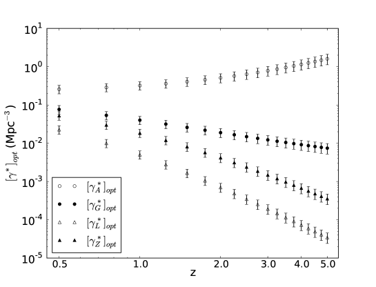
Figure 5: Observational relativistic integral densities versus redshift in the combined optical bands of the FDF dataset of G04. Symbols are as in the legend.

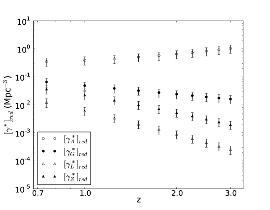
Figure 6: Observational relativistic integral densities versus redshift in the combined red bands of the FDF dataset of G06. Symbols are as in the legend.

The fact that such differential densities depend on the geometry of the Universe through the term inside the brackets of equation (44) causes them to vary with the redshift differently, and they do not necessarily remain constant. Such inhomogeneities, however, are to be understood simply as a consequence of using relativistic distances, defined on the observer’s past light cone. They are therefore easily reconciled with the Cosmological Principle, which requires large-scale spatial homogeneity. As can be seen in figures 5 and 6 of A07, both differential and integral number densities can be inhomogeneous, even when a constant average galaxy mass is assumed in an otherwise spatially homogeneous FLRW metric. Moreover, both quantities calculated using $d_{\scriptscriptstyle G}$ remain homogeneous, as expected, since this distance in this particular spacetime is not affected by expansion, as discussed before.

We can use this important result to further compare the relativistic effects of considering densities down the past light cone in an expanding FLRW spacetime and the observational evolution of the LF in that same hypersurface. The argument is simple: if we compute the ratio of the theoretical values of a given relativistic density at a given redshift – say the differential number density using the luminosity distance $d_{\scriptscriptstyle L}$ – to the one using $d_{\scriptscriptstyle G}$, this indicates how much observational inhomogeneity is introduced through the use of $d_{\scriptscriptstyle L}$ in the calculation of this relativistic density. Similarly, the ratio of the observational value of $[\gamma_{\scriptscriptstyle G}]_{{\textstyle{\scriptscriptstyle obs}}}$ to its theoretical one, $\gamma_{\scriptscriptstyle G}$, indicates how much observational inhomogeneity the redshift evolution of the LF introduces. In fact, considering equations (44) and (54) we can see that such a ratio is simply the completeness function $J(z)$ in a particular dataset, that is,

$$\frac{[\gamma_{\scriptscriptstyle G}]_{{\textstyle{\scriptscriptstyle obs}}}}{\gamma_{\scriptscriptstyle G}} = \frac{[dN/dz]_{{\textstyle{\scriptscriptstyle obs}}}\{4\pi(d_{\scriptscriptstyle G})^{2}\;d(d_{\scriptscriptstyle G})/dz\}^{-1}}{dN/dz\{4\pi(d_{\scriptscriptstyle G})^{2}\;d(d_{\scriptscriptstyle G})/dz\}^{-1}}$$ (69)

$$= \frac{[dN/dz]_{{\textstyle{\scriptscriptstyle obs}}}}{dN/dz}=J(z).$$

Now, if there were no significant departure from homogeneity at a given redshift such ratios should be approximately unity. Therefore, if we subtract the values of those ratios at a given redshift from one, this number should express how much inhomogeneity that relativistic density shows at that redshift: the bigger the number, the bigger the inhomogeneity. Table 6 summarizes these results. At a fixed redshift entry one can compare the effects on the homogeneity of the relativistic differential densities caused by the LF redshift evolution of the different filters in the G04 and G06 datasets.

The results in Table 6 allow us to see that the evolution of the LF in the combined UV bands produces a bigger departure from homogeneity of the differential densities than the one in the combined optical bands, and this departure is even bigger than the one in the combined red ones. On the other hand, fixing a given ratio, say the observational-to-theoretical ratio for the UV bands, $[\gamma_{\scriptscriptstyle G}]_{{\textstyle{\scriptscriptstyle obs}}}/\gamma_{\scriptscriptstyle G}$, one can observe that the departure from homogeneity of these relativistic differential densities is quite a common feature and tends to increase with redshift. Finally, by comparing the values of the purely theoretical $\gamma_{\scriptscriptstyle L}/\gamma_{\scriptscriptstyle G}$ ratio to the various observational-to-theoretical ones, one can investigate which contribution dominates at each redshift. That is particularly interesting, since the redshift evolution of any of the other differential densities can be obtained by a simple combination of those two separate effects, that of the expansion of the geometry in the distance definition and that of the redshift evolution of the LF. For instance, let us consider the observational differential density in the combined UV filters calculated using the luminosity distance $d_{\scriptscriptstyle L}$, that is, $[\gamma_{\scriptscriptstyle L}]_{\scriptscriptstyle UV}$. Its departure from homogeneity can be investigated using the ratio $[\gamma_{\scriptscriptstyle L}]_{\scriptscriptstyle UV}/\gamma_{\scriptscriptstyle G}$, as discussed above. Remembering that, by construction $[\gamma_{\scriptscriptstyle L}]_{\scriptscriptstyle UV}=J_{\scriptscriptstyle UV}\,\gamma_{\scriptscriptstyle L}$, it follows,

$$\frac{[\gamma_{\scriptscriptstyle L}]_{\scriptscriptstyle UV}}{\gamma_{\scriptscriptstyle G}}=\frac{J_{\scriptscriptstyle UV}\,\gamma_{\scriptscriptstyle L}}{\gamma_{\scriptscriptstyle G}}=\frac{[\gamma_{\scriptscriptstyle G}]_{\scriptscriptstyle UV}}{\gamma_{\scriptscriptstyle G}}\frac{\gamma_{\scriptscriptstyle L}}{\gamma_{\scriptscriptstyle G}},$$ (70)

which is simply the combination of the observational-to-theoretical ratio for that dataset, namely the LF of the combined UV bands with the purely theoretical ratio for that distance definition, in that case, $d_{\scriptscriptstyle L}$. The values in Table 6 indicate that the geometrical effect is comparable to the evolution of the LF in the whole redshift range of the G04 and G06 datasets.

At this point, one should note that determining the spacetime geometry of the Universe or its density parameters is not the goal of the present paper. We simply assume the $\Lambda$CDM metric, a necessary step in calculating the above mentioned geometrical terms, in order to see how the empirical evolution of the differential number counts $[dN/dz]_{{\textstyle{\scriptscriptstyle obs}}}$ affects the theoretical results discussed above.

Similarly, we can obtain the observational values of the integral densities $[\gamma]_{{\textstyle{\scriptscriptstyle obs}}}^{\ast}$ by means of equation (46), or (48), because, by their very definitions, we have that $[N]_{{\textstyle{\scriptscriptstyle obs}}}=V_{\scriptscriptstyle C}\;\psi(z)$.

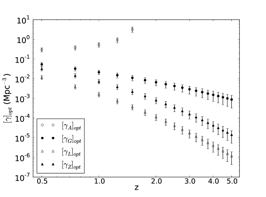
Figure 2: Observational relativistic differential densities versus redshift in the combined optical bands of the FDF dataset of G04. Symbols are as in the legend.

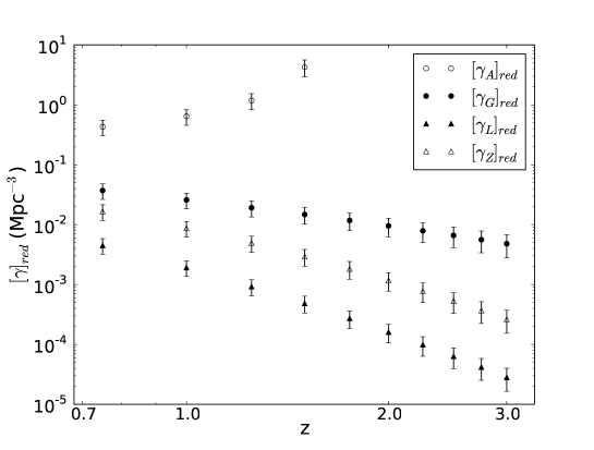
Figure 3: Observational relativistic differential densities versus redshift in the combined red bands of the FDF dataset of G06. Symbols are as in the legend.

Figures 1 and 2 show graphs of the observational differential densities determined using the combined UV and optical bands in the G04 dataset plotted against the redshift, whereas figure 3 shows the results for those same densities versus the redshift in the combined red bands. The dependence of such relativistic densities on the distance definition, a known theoretical result (Ribeiro 2005; A07), can be easily observed in these three figures. In addition, the dependence of $[\gamma_{\scriptscriptstyle G}]_{{\textstyle{\scriptscriptstyle obs}}}$ with the redshift in these same figures is solely due to the evolution of the mass function, since its relativistic volume definition remains constant in the assumed FLRW spacetime. We note that values of $[\gamma_{\scriptscriptstyle G}]_{{\textstyle{\scriptscriptstyle obs}}}$ obtained from the LF in the combined red bands (figure 3) seem less dependent on the redshift than those in the UV and optical bands (figures 1 and 2).

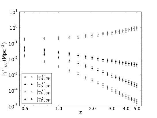
Figure 4: Observational relativistic integral densities versus redshift in the combined UV bands of the FDF dataset of G04. Symbols are as in the legend.

Similar graphs for the observational integral densities in the UV, optical and red combined bands versus the redshift are respectively shown in figures 4, 5, and 6, where their dependency with the distance definition can also be clearly seen. Although less pronounced in these smoothed out relativistic densities, the effect of the evolution of the mass function can still be observed in these three graphs, as $[\gamma^{\ast}_{\scriptscriptstyle G}]_{{\textstyle{\scriptscriptstyle obs}}}$ is also unaffected by the geometrical effects of considering the densities on the past null light cone of an FLRW spacetime. In other words, the LF redshift evolution seems to further enhance the inhomogeneity of these densities, making observationally inhomogeneous even the theoretically homogeneous $\gamma_{\scriptscriptstyle G}$ and $\gamma^{\ast}_{\scriptscriptstyle G}$. We observe that in figure 6, $[\gamma^{\ast}_{\scriptscriptstyle G}]_{{\textstyle{\scriptscriptstyle obs}}}$ is also less dependent on the redshift than in the UV and optical bands shown in figures 4 and 5.

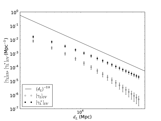
Figure 7: Observational relativistic differential and integral densities versus luminosity distance in the combined UV bands of the FDF dataset of G04. The solid line was drawn just as reference, to show the apparent power-law behavior of both relativistic densities in that distance definition at high redshifts. Symbols are as in the legend.

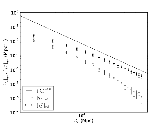
Figure 8: Observational relativistic differential and integral densities versus luminosity distance in the combined optical bands of the FDF dataset of G04. The solid line is plotted just as a reference to the power law behavior stated in the legend. Symbols are as in the legend.

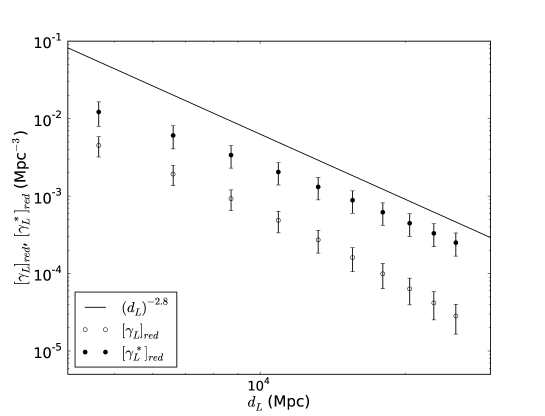
Figure 9: Observational relativistic densities versus luminosity distance in the combined red bands of the FDF dataset of G06. The solid line is shown as a reference to the power law behavior stated in the legend. Symbols are as in the legend.

Figures 7, 8, and 9 plot the observational differential and integral densities built with the luminosity distance in the combined UV, optical and red bands, respectively, versus the luminosity distance. A power-law pattern for both densities in the three combined bands can be observed when one compares the data points with the solid line drawn just as reference in all three plots. The slope of the reference lines is the same in all bands, which indicates that there is little change in the slope of the data points. This possibly indicates that such an effect is predominantly relativistic.

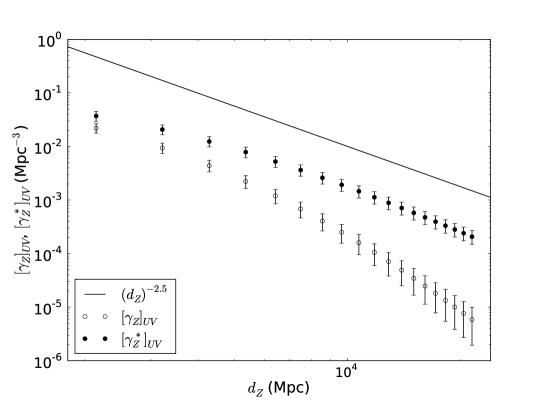
Figure 10: Observational relativistic differential and integral densities versus redshift distance in the combined UV bands of the FDF dataset of G04. The solid line is shown just as a reference to the power law behavior stated in the legend. Symbols are as in the legend.

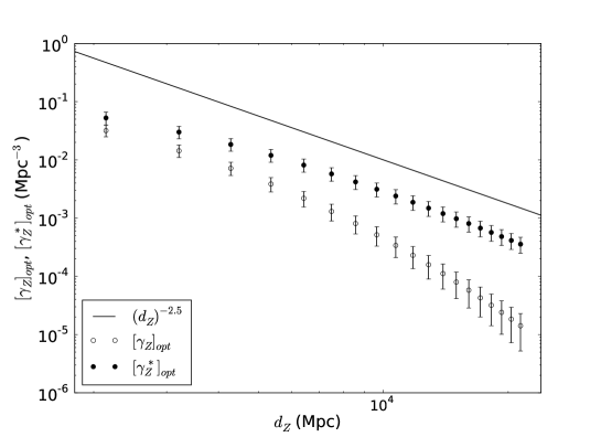
Figure 11: Observational relativistic differential and integral densities versus redshift distance in the combined optical bands of the FDF dataset of G04. The solid line is shown as a reference to the power law behavior stated in the legend. Symbols are as in the legend.

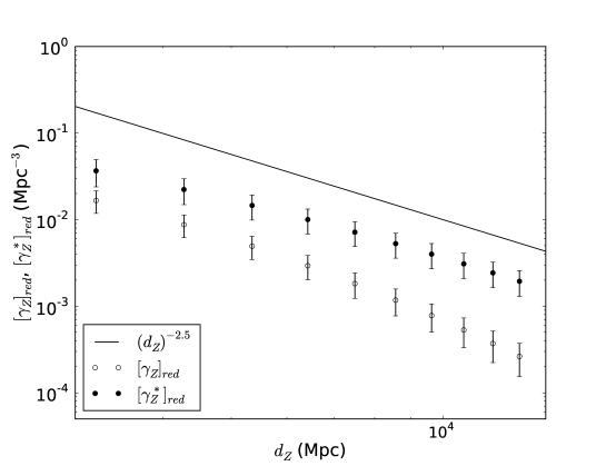
Figure 12: Observational relativistic differential and integral densities versus redshift distance in the combined red bands of the FDF dataset of G06. The solid line is plotted as a reference to the power law behavior stated in the legend. Symbols are as in the legend.

A similar pattern can be found in figures 10, 11, and 12, which plot the observational differential and integral densities using the redshift distance against that same distance in the combined UV, optical and red bands respectively. We found a similar indication of a power-law pattern in both densities at high redshifts, but the actual power exponent of the distributions is different from the one using the luminosity distance. This comes from the fact that these two relativistic distances are affected differently by the expansion of the FLRW spacetime. Comparing the results shown in figure 11 with the ones in the UV band in figure 10 we can see that the slopes of the data points should agree with one another. Similarly as in figures 10 and 11, the power law exponent shown in figure 12 seems to be the same for both $[\gamma_{\scriptscriptstyle Z}]_{{\textstyle{\scriptscriptstyle obs}}}$ and $[\gamma^{\ast}_{\scriptscriptstyle Z}]_{{\textstyle{\scriptscriptstyle obs}}}$ in the given distance definition.

One should notice that the slope of the straight lines used as references for the data points in figures 7 to 12 do not vary drastically over all bands of the FDF datasets, both for luminosity and redshift distance definitions. This possibly indicates that such an effect is predominantly relativistic.

The differential density constructed with the area distance $d_{\scriptscriptstyle A}$ becomes discontinuous at $z\approx 1.5$ due to the fact that, by definition, $d_{\scriptscriptstyle A}$ has a maximum at that redshift and, therefore, its derivative with respect to $z$ becomes zero, yielding an undefined $[\gamma_{\scriptscriptstyle A}]_{{\textstyle{\scriptscriptstyle obs}}}$ at high redshifts. In addition, differently from the decrease of $\gamma^{\ast}_{\scriptscriptstyle L}$ and $\gamma^{\ast}_{\scriptscriptstyle Z}$ at higher redshifts, the integral density $\gamma^{\ast}_{\scriptscriptstyle A}$ increases with $z$. Such pathologies have already been previously detected (see figs. 5 and 6 of A07). They seem to render the number densities defined by $d_{\scriptscriptstyle A}$ as unphysical.

The differential and integral densities defined by $d_{\scriptscriptstyle G}$ lack the geometrical effect of expansion in the particular spacetime under consideration in this paper and, therefore, are understood to be unsuitable if one wants to fully characterize the relativistic power-law patterns arising from the combination of both spacetime expansion and LF evolution.

Finally, it is apparent that the differential densities $[\gamma_{\scriptscriptstyle L}]_{{\textstyle{\scriptscriptstyle obs}}}$ and $[\gamma_{\scriptscriptstyle z}]_{{\textstyle{\scriptscriptstyle obs}}}$ do not appear to exhibit a power-law decay as the integral ones do, especially at redshift values nearing the sample’s depth. This is very similar to what found in A07. This behavior is possibly a result of noisier data at the redshift limit of the samples. By definition, the differential densities measure the rate of growth in number counts, rendering them more sensitive to local fluctuations, whereas the integral densities indicate the change in number counts for entire observational volumes, rendering them less sensitive to the same fluctuations.

The indication of power-law behavior may be the result of observational, not necessarily spatial, inhomogeneity as we look down our past light cone, combined with the incompleteness of galaxy counts at higher redshifts. It may also be a result of other causes which we are investigating.

6 Conclusion

In this paper we have detailed a generalization of the framework connecting the relativistic cosmology number count theory with the astronomical data extracted from the galaxy luminosity function (LF), as proposed by Ribeiro & Stoeger (2003). This framework was used by Albani et al. (2007) to extract the observed differential number counts from the LF data and to study the observational inhomogeneities in the relativistic radial densities using different distance definitions. Here we have carried out an analysis of number counts using the LF dataset of Gabasch et al. (2004) in the redshift range $0.5\leq z\leq 5.0$, and of Gabasch et al. (2006) in the redshift range $0.75\leq z\leq 3.0$. In doing so we focused on the observational inhomogeneities in the relativistic radial statistics of the distribution of the galaxies by means of the differential densities $\gamma_{\scriptscriptstyle i}$ ($i={\scriptstyle A}$, ${\scriptstyle G}$, ${\scriptstyle L}$, ${\scriptstyle Z}$) and integral densities $\gamma^{\ast}_{\scriptscriptstyle i}$, both using the various cosmological distance definitions $d_{i}$, as well as the selection functions and the differential number counts $[dN/dz]_{{\textstyle{\scriptscriptstyle obs}}}$ obtained from the LF of G04 and G06.

We confirmed the dependence of such empirically based relativistic densities on the distance definition, a geometrical consequence of the expansion of the Universe, which also is the cause of the observational inhomogeneities present even in theoretical analysis of the spatially homogeneous FLRW spacetime. Furthermore, as expected, the effect of the redshift evolution of the LF seems to increase the observational inhomogeneity of these densities.

We found evidence of a power-law pattern in the behavior of $[\gamma_{\scriptscriptstyle L}]_{{\textstyle{\scriptscriptstyle obs}}}$ and $[\gamma_{\scriptscriptstyle z}]_{{\textstyle{\scriptscriptstyle obs}}}$, relative to their respective cosmological distance measures $d_{\scriptscriptstyle L}$ and $d_{\scriptscriptstyle G}$, similar to that previously detected in A07. However, this pattern is somewhat less pronounced than the results of A07. This difference could be due to the use of a different, and somewhat more complete, redshift samples used in this paper, especially the red galaxies of G06.

Finally, we should note the dependence of these results and their interpretation on the assumed FLRW cosmology. Therefore, we look forward to finding out what an analysis of this data with reference to an inhomogeneous cosmological model (e.g., a Lemaître-Tolman-Bondi model) would reveal. If the universe is not almost-FLRW or if the data are not probing almost-FLRW scales, then hidden in the results are the effects of having chosen the wrong cosmological model. In addition, what we interpret as LF evolution, which is the same as number evolution, but with some indirect luminosity evolution effects, undoubtedly also reflects a lot of unobserved, and therefore uncounted, galaxies. Strictly speaking, if the differential and integral densities are comoving densities, then $\gamma_{\scriptscriptstyle G}$ and $\gamma^{\ast}_{\scriptscriptstyle G}$ should increase with redshift, as there should be more galaxies in a comoving volume in the past that there are now due to mergers (more, but smaller, galaxies in the past). So we are obviously not observing as many galaxies as we go farther out. Of course, that would mean that the average mass per galaxy decreases with redshift, an effect that should be implicit in the empirical LF, but which requires further theoretical considerations to be made explicit in our model. Including these points in our general approach to the problem of connecting relativistic cosmology theory and the empirically determined LF is indeed necessary in order to make the present study even more realistic. We intend to deal with these issues, as well as others like the possible meaning of power law patterns in the differential and integral densities, in forthcoming papers.

Acknowledgments: Thanks go to A. Gabasch for kindly providing the absolute magnitudes of their I-band selected dataset and thoroughly helping us with its observational details. We are also grateful to the referee for providing very helpful criticisms, recommendations and remarks which substantially improved the paper. Finally, we thank M. Giavalisco for some clarifying discussions.

Table 1: Comparison with previous works

Subject	RS03	A07	This work
redshift range	$0.05\rightarrow 1.0$	$0.05\rightarrow 1.0$	$0.5\rightarrow 5.0$
cosmology	EdS	FLRW	FLRW
classification	none	none	UV, optical, red
methodology	J implicit	FLRW implicit	J, FLRW clarified

Table 2: Selection functions for the FDF blue UV bands

redshift	$\psi^{\scriptscriptstyle 1500}$		$\psi^{\scriptscriptstyle 2800}$		$\psi^{\scriptscriptstyle u^{\prime}}$
	($10^{-3}$ Mpc-3)		($10^{-3}$ Mpc-3)		($10^{-3}$ Mpc-3)
0.50	31.0	${}^{+6.9}_{-5.9}$	37.5	${}^{+7.9}_{-7.7}$	42.7	${}^{+9.1}_{-7.9}$
0.75	16.4	${}^{+4.1}_{-3.6}$	21.2	${}^{+4.9}_{-4.8}$	25.2	${}^{+5.6}_{-5.0}$
1.00	9.6	${}^{+2.7}_{-2.4}$	13.2	${}^{+3.4}_{-3.3}$	16.2	${}^{+3.9}_{-3.5}$
1.25	6.1	${}^{+1.9}_{-1.7}$	8.8	${}^{+2.5}_{-2.5}$	11.1	${}^{+2.9}_{-2.6}$
1.50	4.1	${}^{+1.4}_{-1.3}$	6.1	${}^{+1.9}_{-1.9}$	8.0	${}^{+2.2}_{-2.1}$
1.75	2.8	${}^{+1.1}_{-1.0}$	4.5	${}^{+1.5}_{-1.5}$	5.9	${}^{+1.8}_{-1.7}$
2.00	2.05	${}^{+0.87}_{-0.80}$	3.3	${}^{+1.3}_{-1.3}$	4.5	${}^{+1.5}_{-1.4}$
2.25	1.53	${}^{+0.71}_{-0.65}$	2.6	${}^{+1.0}_{-1.1}$	3.5	${}^{+1.2}_{-1.2}$
2.50	1.16	${}^{+0.58}_{-0.54}$	2.02	${}^{+0.88}_{-0.89}$	2.80	${}^{+1.04}_{-0.99}$
2.75	0.91	${}^{+0.49}_{-0.46}$	1.62	${}^{+0.76}_{-0.77}$	2.26	${}^{+0.90}_{-0.85}$
3.00	0.72	${}^{+0.41}_{-0.39}$	1.32	${}^{+0.65}_{-0.66}$	1.85	${}^{+0.78}_{-0.74}$
3.25	0.58	${}^{+0.35}_{-0.33}$	1.09	${}^{+0.57}_{-0.58}$	1.54	${}^{+0.69}_{-0.65}$
3.50	0.48	${}^{+0.30}_{-0.29}$	0.91	${}^{+0.50}_{-0.51}$	1.29	${}^{+0.61}_{-0.58}$
3.75	0.40	${}^{+0.27}_{-0.25}$	0.76	${}^{+0.45}_{-0.46}$	1.09	${}^{+0.54}_{-0.51}$
4.00	0.33	${}^{+0.23}_{-0.22}$	0.65	${}^{+0.40}_{-0.41}$	0.93	${}^{+0.49}_{-0.46}$
4.25	0.28	${}^{+0.21}_{-0.20}$	0.56	${}^{+0.36}_{-0.37}$	0.80	${}^{+0.44}_{-0.41}$
4.50	0.24	${}^{+0.18}_{-0.17}$	0.48	${}^{+0.32}_{-0.33}$	0.70	${}^{+0.40}_{-0.37}$
4.75	0.21	${}^{+0.16}_{-0.16}$	0.42	${}^{+0.29}_{-0.30}$	0.61	${}^{+0.36}_{-0.34}$
5.00	0.18	${}^{+0.15}_{-0.14}$	0.37	${}^{+0.27}_{-0.27}$	0.53	${}^{+0.33}_{-0.31}$

Table 3: Selection functions for FDF blue optical bands

redshift	$\psi^{\scriptscriptstyle g^{\prime}}$		$\psi^{\scriptscriptstyle B}$
	($10^{-3}$ Mpc-3)		($10^{-3}$ Mpc-3)
0.50	55	${}^{+14}_{-12}$	53	${}^{+13}_{-11}$
0.75	32.7	${}^{+8.5}_{-7.7}$	31.4	${}^{+7.7}_{-7.2}$
1.00	21.7	${}^{+6.0}_{-5.5}$	20.7	${}^{+5.4}_{-5.1}$
1.25	15.3	${}^{+4.6}_{-4.2}$	14.6	${}^{+4.0}_{-3.9}$
1.50	11.3	${}^{+3.6}_{-3.3}$	10.7	${}^{+3.2}_{-3.1}$
1.75	8.6	${}^{+2.9}_{-2.7}$	8.2	${}^{+2.6}_{-2.5}$
2.00	6.8	${}^{+2.5}_{-2.3}$	6.3	${}^{+2.1}_{-2.1}$
2.25	5.4	${}^{+2.1}_{-1.9}$	5.0	${}^{+1.8}_{-1.8}$
2.50	4.4	${}^{+1.8}_{-1.7}$	4.1	${}^{+1.5}_{-1.6}$
2.75	3.6	${}^{+1.6}_{-1.5}$	3.3	${}^{+1.3}_{-1.4}$
3.00	3.0	${}^{+1.4}_{-1.3}$	2.8	${}^{+1.1}_{-1.2}$
3.25	2.5	${}^{+1.2}_{-1.2}$	2.3	${}^{+1.0}_{-1.1}$
3.50	2.1	${}^{+1.1}_{-1.0}$	1.96	${}^{+0.89}_{-0.95}$
3.75	1.84	${}^{+0.98}_{-0.92}$	1.67	${}^{+0.80}_{-0.85}$
4.00	1.59	${}^{+0.88}_{-0.83}$	1.43	${}^{+0.71}_{-0.76}$
4.25	1.37	${}^{+0.80}_{-0.76}$	1.23	${}^{+0.64}_{-0.69}$
4.50	1.20	${}^{+0.73}_{-0.69}$	1.07	${}^{+0.58}_{-0.63}$
4.75	1.05	${}^{+0.66}_{-0.63}$	0.93	${}^{+0.53}_{-0.57}$
5.00	0.92	${}^{+0.61}_{-0.58}$	0.81	${}^{+0.48}_{-0.52}$

Table 4: Selection functions for the FDF red bands

redshift	$\psi^{\scriptscriptstyle r^{\prime}}$		$\psi^{\scriptscriptstyle i^{\prime}}$		$\psi^{\scriptscriptstyle z^{\prime}}$
	($10^{-3}$ Mpc-3)		($10^{-3}$ Mpc-3)		($10^{-3}$ Mpc-3)
0.75	31.6	${}^{+8.6}_{-8.6}$	35.9	${}^{+9.8}_{-9.9}$	44	${}^{+14}_{-14}$
1.00	22.4	${}^{+6.2}_{-6.2}$	25.0	${}^{+6.8}_{-6.8}$	30.2	${}^{+9.8}_{-9.7}$
1.25	16.8	${}^{+4.8}_{-4.8}$	18.5	${}^{+5.1}_{-5.2}$	22.1	${}^{+7.3}_{-7.3}$
1.50	13.1	${}^{+3.9}_{-3.9}$	14.2	${}^{+4.1}_{-4.1}$	16.9	${}^{+5.8}_{-5.8}$
1.75	10.5	${}^{+3.3}_{-3.3}$	11.3	${}^{+3.4}_{-3.4}$	13.4	${}^{+4.8}_{-4.8}$
2.00	8.6	${}^{+2.9}_{-2.8}$	9.1	${}^{+2.9}_{-2.9}$	10.8	${}^{+4.0}_{-4.1}$
2.25	7.2	${}^{+2.5}_{-2.5}$	7.5	${}^{+2.5}_{-2.5}$	8.9	${}^{+3.5}_{-3.5}$
2.50	6.1	${}^{+2.3}_{-2.2}$	6.3	${}^{+2.2}_{-2.2}$	7.5	${}^{+3.0}_{-3.1}$
2.75	5.2	${}^{+2.1}_{-2.0}$	5.3	${}^{+1.9}_{-2.0}$	6.3	${}^{+2.7}_{-2.7}$
3.00	4.5	${}^{+1.9}_{-1.8}$	4.5	${}^{+1.7}_{-1.7}$	5.4	${}^{+2.4}_{-2.4}$

Table 5: Differential number counts

redshift	$[dN/dz]_{\scriptscriptstyle UV}$		$[dN/dz]_{\scriptscriptstyle opt}$		$[dN/dz]_{\scriptscriptstyle red}$
	($10^{9}$)		($10^{9}$)		($10^{9}$)
0.50	5.4	${}^{+1.2}_{-1.1}$	7.9	${}^{+1.9}_{-1.7}$	—
0.75	5.2	${}^{+1.2}_{-1.1}$	8.0	${}^{+2.0}_{-1.8}$	9.2	${}^{+2.7}_{-2.7}$
1.00	4.3	${}^{+1.1}_{-1.0}$	7.1	${}^{+1.9}_{-1.8}$	8.6	${}^{+2.5}_{-2.5}$
1.25	3.44	${}^{+0.96}_{-0.91}$	5.9	${}^{+1.7}_{-1.6}$	7.6	${}^{+2.3}_{-2.3}$
1.50	2.67	${}^{+0.82}_{-0.78}$	4.9	${}^{+1.5}_{-1.4}$	6.5	${}^{+2.0}_{-2.0}$
1.75	2.07	${}^{+0.69}_{-0.66}$	3.9	${}^{+1.3}_{-1.2}$	5.5	${}^{+1.8}_{-1.8}$
2.00	1.61	${}^{+0.58}_{-0.56}$	3.2	${}^{+1.1}_{-1.1}$	4.6	${}^{+1.6}_{-1.6}$
2.25	1.26	${}^{+0.49}_{-0.47}$	2.58	${}^{+0.96}_{-0.93}$	3.9	${}^{+1.4}_{-1.4}$
2.50	0.99	${}^{+0.41}_{-0.40}$	2.10	${}^{+0.82}_{-0.81}$	3.3	${}^{+1.2}_{-1.2}$
2.75	0.79	${}^{+0.35}_{-0.34}$	1.71	${}^{+0.71}_{-0.70}$	2.8	${}^{+1.1}_{-1.1}$
3.00	0.63	${}^{+0.30}_{-0.29}$	1.41	${}^{+0.61}_{-0.61}$	2.34	${}^{+0.97}_{-0.97}$
3.25	0.51	${}^{+0.26}_{-0.25}$	1.16	${}^{+0.53}_{-0.53}$	—
3.50	0.42	${}^{+0.22}_{-0.22}$	0.96	${}^{+0.47}_{-0.46}$	—
3.75	0.34	${}^{+0.19}_{-0.19}$	0.80	${}^{+0.41}_{-0.41}$	—
4.00	0.29	${}^{+0.17}_{-0.16}$	0.67	${}^{+0.36}_{-0.36}$	—
4.25	0.24	${}^{+0.15}_{-0.14}$	0.57	${}^{+0.31}_{-0.32}$	—
4.50	0.20	${}^{+0.13}_{-0.12}$	0.48	${}^{+0.28}_{-0.28}$	—
4.75	0.17	${}^{+0.11}_{-0.11}$	0.41	${}^{+0.25}_{-0.25}$	—
5.00	0.145	${}^{+0.100}_{-0.097}$	0.35	${}^{+0.22}_{-0.22}$	—

Table 6: Spacetime expansion vs. galaxy evolution effects on relativistic homogeneity

Ratio	$z=1$	$z=3$	$z=5$
1-($\gamma_{\scriptscriptstyle L}$/$\gamma_{\scriptscriptstyle G}$)	0.926	0.9942	0.9987
1-($[\gamma_{\scriptscriptstyle G}]_{\scriptscriptstyle UV}$/$\gamma_{\scriptscriptstyle G}$)	0.969	0.9969	0.9991
1-($[\gamma_{\scriptscriptstyle G}]_{\scriptscriptstyle opt}$/$\gamma_{\scriptscriptstyle G}$)	0.949	0.9930	0.9880
1-($[\gamma_{\scriptscriptstyle G}]_{\scriptscriptstyle red}$/$\gamma_{\scriptscriptstyle G}$)	0.938	0.9880	—

Appendix A Numerical algorithm

This appendix describes step by step how to apply the theoretical and numerical methodologies described in sections §2, §3 and §4 in order to obtain the results used in this paper. Steps 1 to 6 involve the calculation of the theoretical quantities, as discussed in §2 and §3. Steps 7 to 10 show how to obtain the corresponding observational quantities for a given LF, as discussed in §4.

Step 1 – Coupled differential equations. Obtain the scale factor $S(r)$ and the cumulative number count $N(r)$ as a function of the radial coordinate, or comoving distance $r$, by solving the coupled equations (20) and (23). We used the fourth order Runge-Kutta method to obtain values of $S(r)$ and $N(r)$ at fixed $r$ increments, assuming as initial conditions $N(0)=0$ and $S(0)=1$;

Step 2 – Auxiliary quantities. Obtain the redshift $z(r)$ for each increment of $r$ using equation (24) and the corresponding value of the scale factor $S(r)$. Do the same for the area distance $d_{\scriptscriptstyle A}(r)$ using equation (19), the differential number count $dN/dz(r)$ using equation (28), and the comoving volume number density $n_{\scriptscriptstyle C}(r)$ using equation (52);

Step 3 – Cosmological distances. Having the values of $z(r)$ and $d_{\scriptscriptstyle A}(r)$ calculated for each $r$ increment, obtain the values of the galaxy area distance $d_{\scriptscriptstyle G}(r)$, and the luminosity distance $d_{\scriptscriptstyle L}(r)$ by direct application of equation (30), Etherington’s reciprocity law itself. The values of the redshift distance $d_{z}(r)$ can be easily obtained for each $r$ increment using equation (31);

Step 4 – Derivatives of the distances with respect to redshift. For each $r$ increment, calculate the values of the derivatives with respect to redshift of the distances obtained in the previous step by means of equations (36), (39) and (40);

Step 5 – Theoretical differential densities. Obtain the values of the theoretical differential densities $\gamma_{\scriptscriptstyle i}(r)$ for each of the distance definitions $d_{i}$ ($i={\scriptstyle A},{\scriptstyle G},{\scriptstyle L},{\scriptstyle Z}$) calculated previously for each $r$ increment, by means of equation (44);

Step 6 – Theoretical integral densities. Calculate for each distance $d_{\scriptscriptstyle i}(r)$ entry its corresponding spherical volume $V_{\scriptscriptstyle i}(r)$, by means of equations (43), then use those values, together with the ones for the cumulative number count $N(r)$, to obtain the values of the integrated differential densities $\gamma^{\ast}_{\scriptscriptstyle i}(r)$, by means of equation (48);

Step 7 – Selection functions. Select a bin containing a group of redshift values in a certain interval $[z_{a\rightarrow b}]$, from a point $z_{a}$ to a point $z_{b}$, taken from the ones obtained in step 2, and obtain the corresponding values of the selection functions $\psi^{\scriptscriptstyle W}(z_{a\rightarrow b})$ for each filter $W$ using equation (4.2), with the appropriate values for the LF’s Schechter parameters $\phi^{\ast}(z_{a\rightarrow b})$, $M^{\ast}(z_{a\rightarrow b})$, and $\alpha(z_{a\rightarrow b})$, and different absolute magnitude limits $M^{\scriptscriptstyle W}_{lim}(z_{a\rightarrow b})$, given by equation (65);

Step 8 – Completeness functions. Calculate the values of the completeness function $J^{\scriptscriptstyle W}(z_{a\rightarrow b})$ by means of equation (50) using the selection functions $\psi^{\scriptscriptstyle W}(z_{a\rightarrow b})$ calculated in step 7 and the corresponding values of the comoving volume number density $n_{\scriptscriptstyle C}[z_{a\rightarrow b}(r)]$ obtained in step 2;

Step 9 – Differential and cumulative number counts. Obtain the observational differential number count $[dN/dz]_{{\textstyle{\scriptscriptstyle obs}}}^{\scriptscriptstyle W}(z_{a\rightarrow b})$ in each filter $W$ by means of equation (54) and the observational cumulative number count $[N]_{{\textstyle{\scriptscriptstyle obs}}}^{\scriptscriptstyle W}(z_{a\rightarrow b})$, by means of equation (66);

Step 10 – Observational differential and integral densities. Obtain the observational differential densities $[\gamma_{\scriptscriptstyle i}]_{{\textstyle{\scriptscriptstyle obs}}}^{\scriptscriptstyle W}(z_{a\rightarrow b})$, and the integrated differential densities $[\gamma^{\ast}_{\scriptscriptstyle i}]_{{\textstyle{\scriptscriptstyle obs}}}^{\scriptscriptstyle W}(z_{a\rightarrow b})$, by using the values of $[dN/dz]_{{\textstyle{\scriptscriptstyle obs}}}^{\scriptscriptstyle W}(z_{a\rightarrow b})$ and $[N]_{{\textstyle{\scriptscriptstyle obs}}}^{\scriptscriptstyle W}(z_{a\rightarrow b})$ in place of their theoretical counterparts $dN/dz$ and $N$ in equations (44) and (48), respectively.

References

- (1) Albani, V. V. L., Iribarrem, A. S., Ribeiro, M. B., and Stoeger, W. R. 2007, ApJ, 657, 760; astro-ph/0611032, (A07)
- (2) Bell, E. F., Mcintosh, D. H., Katz, N., and Weinberg, M. D. 2003, ApJS, 149, 289
- (3) Blanton, M. R., Hogg, D. W., Bahcall, N. A., Brinkmann, J. et al. 2003, ApJ, 592, 819
- (4) Bouwens, R. J., Illingworth, G. D., Franx, M., and Ford, H. 2007, ApJ, 670, 928
- (5) Ellis, G. F. R. 1971, in General Relativity and Cosmology, ed. R. K. Sachs (Proc. Int. School Phys. “Enrico Fermi”; New York: Academic Press); reprinted in Gen. Rel. Grav., 41, 581, 2009
- (6) Ellis, G. F. R. 2007, Gen. Rel. Grav., 39, 1047
- (7) Etherington, I. M. H. 1933, Phil. Mag. ser. 7, 15, 761; reprinted in Gen. Rel. Grav. 39, 1055, 2007
- (8) Fried, J. W., von Kuhlmann, B., Meisenheimer, K., Rix, H.-W. et al. 2001, A&A, 367, 788
- (9) Gabasch, A., Bender, R., Seitz, S., Hopp, U. et al. 2004, A&A, 421, 41 (G04)
- (10) Gabasch, A., Hopp, U., Feulner, G., Bender, R. et al. 2006, A&A, 448, 101 (G06)
- (11) Gabasch, A., Goranova, Y., Hopp, U., Noll, S. et al. 2008, MNRAS, 383, 1319
- (12) Heidt, J., Appenzeller, I., Bender, R., Böhm, A. et al. 2001, The FORS Deep Field, Reviews in Modern Astronomy, Vol. 14, R.E. Schielicke (Ed.), Astronomische Gesellschaft
- (13) Lin, H., Yee, H. K. C., Carlberg, R. G., Morris, S. L. et al. 1999, ApJ, 518, 533
- (14) Ly, C., Malkan, M. A., Kashikawa, N., Shimasaku, K. et al. 2007, ApJ, 657, 738
- (15) Norman, C., Ptak, A., Hornschemeier, A., Hasinger, G. et al. 2004, ApJ, 607, 721
- (16) Peacock, J. A. 1999, Cosmological Physics (Cambridge: Cambridge Univ. Press)
- (17) Plebański, J., & Krasiński, A. 2006, An Introduction to General Relativity and Cosmology (Cambridge University Press)
- (18) Poli, F., Giallongo, E., Fontana, A., Menci, N. et al. , ApJ, 593, L1
- (19) Pozzetti, L., Cimatti, A., Zamorani, G., Daddi, E. et al. 2003, A&A, 402, 837
- (20) Rangel Lemos, L. J., and Ribeiro, M. B. 2008, A&A, 488, 55; arXiv:0805.3336
- (21) Ribeiro, M. B. 1992, ApJ, 395, 29; arXiv:0807.0869
- (22) Ribeiro, M. B. 1995, ApJ, 441, 477; astro-ph/9910145
- (23) Ribeiro, M. B. 2001, Gen. Rel. Grav., 33, 1699; astro-ph/0104181
- (24) Ribeiro, M. B. 2005, A&A, 429, 65; astro-ph/0408316
- (25) Ribeiro, M. B., and Stoeger, W. R. 2003, ApJ, 592, 1; astro-ph/0304094, (RS03)
- (26) Roos, M., Introduction to Cosmology, Chichester: Wiley, 1994
- (27) Rudnick, G., Rix, H.-W., Franx, M., Labbé, I. et al. 2003, ApJ, 599, 847
- (28) Schechter, P. 1976, ApJ, 203, 297
- (29) Sparke, L.S., and Gallagher, J.S. 2000, Galaxies in the Universe (Cambridge University Press)
- (30) Stoeger, W. R., Ellis, G. F. R., and Nel, S. D. 1992, Class. Q. Grav., 9, 509
- (31) Tzanavaris, P., and Georgantopoulos, I. 2008, A&A, 480, 663
- (32) Wilmer, C. N. A., Faber, S. M., Koo, D. C., Weiner, B. J. et al. 2006, ApJ, 647, 853