Modifying the Casimir force between indium tin oxide film and Au sphere

Abstract

We present complete results of the experiment on measuring the Casimir force between an Au-coated sphere and an untreated or, alternatively, UV-treated indium tin oxide film deposited on a quartz substrate. Measurements were performed using an atomic force microscope in a high vacuum chamber. The measurement system was calibrated electrostatically. Special analysis of the systematic deviations is performed, and respective corrections in the calibration parameters are introduced. The corrected parameters are free from anomalies discussed in the literature. The experimental data for the Casimir force from two measurement sets for both untreated and UV-treated samples are presented. The random, systematic and total experimental errors are determined at a 95% confidence level. It is demonstrated that the UV treatment of an ITO plate results in a significant decrease in the magnitude of the Casimir force (from 21% to 35% depending on separation). However, ellipsometry measurements of the imaginary parts of dielectric permittivities of the untreated and UV-treated samples did not reveal any significant differences. The experimental data are compared with computations in the framework of the Lifshitz theory. It is found that the data for the untreated sample are in a very good agreement with theoretical results taking into account the free charge carriers in an ITO film. For the UV-treated sample the data exclude the theoretical results obtained with account of free charge carriers. These data are in a very good agreement with computations disregarding the contribution of free carriers in the dielectric permittivity. According to the hypothetical explanation provided, this is caused by the phase transition of the ITO film from metallic to dielectric state caused by the UV-treatment. Possible applications of the discovered phenomenon in nanotechnology are discussed.

I Introduction

Widespread interest in the van der Waals and Casimir forces (see recent monographs1 ; 2 ; 3 ; 4 ; 5 ; 6 and reviews7 ; 8 ; 9 ; 10 ; 11 ; 12 ) is from the key role they play in many physical phenomena ranging from condensed matter physics to gravitation and cosmology. It is common knowledge that the van der Waals force is of quantum nature and originates from fluctuations of the electromagnetic field. Casimir13 was the first to generalize the van der Waals force bewtween two macrobodies to separations where the effects of relativistic retardation become important. The corresponding generalization of the van der Waals interaction between an atom and a cavity wall was performed by Casimir and Polder.14 Both the van der Waals and Casimir forces are known under the generic name dispersion forces. In fact, the attractive dispersion forces between two macrobodies, between a polarizable particle and a macrobody and between two particles become dominant when separation distances shrink below a micrometer. That is why these forces are of great importance in nanotechnology where they can play the useful role of a driving force which actuates a microelectromechanical device.15 ; 16 Conversely, dispersion forces may be harmful leading to a stable state of stiction, i.e., adhesion of free parts of a microdevice to neighboring substrates or electrodes.17 ; 18

A large body of experimental and theoretical research is devoted to the problem of how to control the magnitude and sign of the Casimir force. In regard to the Casimir force with an opposite sign (the so-called Casimir repulsion), it was possible to qualitatively demonstrate it12 only in the case of two material bodies separated with a liquid layer, as predicted by the Lifshitz theory.5 ; 6 ; 19 Experiments on modifying the magnitude of the attractive Casimir force are numerous and varied. They are based on the idea that modification of the optical properties of the test bodies should lead to changes in the force in accordance with the Lifshitz theory. The Casimir force takes the largest magnitude when both test bodies are made of good metal, e.g., of Au, which is characterized by high reflectivity over a wide frequency region. It was demonstrated20 ; 21 ; 22 that the Casimir force between an Au sphere and a Si plate is smaller by 25%–40% than in the case of two Au bodies. This was explained by the fact that the dielectric permittivity of Si along the imaginary frequency axis is much smaller than that of Au. For an indium tin oxide (ITO, In₂O₃:Sn) film interacting with an Au sphere the gradient of the Casimir force was measured23 ; 24 to be roughly 40%–50% smaller than between an Au sphere and an Au plate. In one more experiment25 it was shown that for an Au sphere interacting with a plate made of AgInSbTe the gradient of the Casimir force decreases in magnitude by approximately 20% when the material of the plate in the crystalline phase is replaced with an amorphous one. For a semimetallic plate, the gradient of the Casimir force was reported to be 25%–35% smaller than for an Au plate.26

Keeping in mind the applications to micromachines, it is important to control both decreases and increases in the force magnitude. For this purpose, the difference in the Casimir force between a Si plate and an Au sphere was measured27 ; 28 in the presence and in the absence of 514 nm Ar laser light on the plate. The respective increase in magnitude of the Casimir force by a few percent was observed when the plate is illuminated with laser pulses. This was explained by an increase in the charge carrier density up to five orders of magnitude under the influence of light and respective changes in the dielectric permittivity of the plate.

Investigation of the Casimir force between different materials not only led to important experimental results with potential applications in nanotechnology, but also raised unexpected theoretical problems touching on the foundations of quantum statistical physics. Thus, for two metal test bodies (an Au-coated sphere of 150 $\mu$m radius above an Au-coated plate) the measured gradient of the Casimir force at laboratory temperature was found to be in agreement with the Lifshitz theory of dispersion forces only if the relaxation properties of free charge carriers (electrons) are disregarded.29 ; 30 If these relaxation properties were taken into account by means of the Drude model, the Lifshitz theory was found to be excluded by the experimental data at almost 100% confidence level. Recently it was claimed31 that an experiment using an Au-coated spherical lens of 15.6 cm curvature radius above an Au-coated plate is in agreement with theory taking into account the relaxation properties of free electrons. The results of this experiment are in contradiction with the above mentioned measurement using a small sphere29 ; 30 and another experiment using large spherical lens.32 (See Refs.33 ; 34 for detailed critical discussion.)

For an Au sphere interacting with a Si plate illuminated with laser pulses the experimental data for the difference in the Casimir forces in the presence and in the absence of light agree with the Lifshitz theory only if the charge carriers of dielectric Si in the absence of light are disregarded.27 ; 28 When the charge carriers are taken into account, the Lifshitz theory is excluded by the data at a 95% confidence level. Similar results were obtained from the measurement35 of the thermal Casimir-Polder force between ⁸⁷Rb atoms belonging to the Bose-Einstein condensate and a SiO₂ plate: theory is in agreement with the data when dc conductivity of the dielectric plate is disregarded,35 but the same theory is excluded by the data at a 70% confidence level when dc conductivity is taken into account.36

In this paper, we present complete experimental and theoretical results for the Casimir force between an Au-coated sphere and ITO films deposited on a quartz substrate. Measurements were performed using a modified multimode atomic force microscope (AFM) in high vacuum. The main difference of this experiment in comparison with Refs.23 ; 24 is that in two sets of measurements the ITO sample was used as is, but another two sets of measurements were done after the sample was subjected to UV treatment. Unexpectedly, it was observed that the UV treatment results in a significant decrease in the magnitude of the Casimir force (from 21% to 35% at different separations). This decrease is not associated with respective modifications of the optical properties of plates under the influence of UV treatment, as was confirmed by means of ellipsometry measurements (preliminary results of this work based on only one data set were published in Ref.38 ).

The experimental results are compared with calculations using the Lifshitz theory and different models of the dielectric properties of the test bodies. Note that ITO at room temperature is a good conductor at quasistatic frequencies, but is transparent to visible and near infrared light. Keeping this in mind, it was suggested39 to use this material in investigations of the Casimir force. Computations are done for a four-layer system (ITO on quartz interacting with Au through a vacuum gap). The experimental results for an untreated ITO sample are found to be in agreement with the Lifshitz theory if charge carriers are taken into account. For a UV-treated sample, the Lifshitz theory taking into account the charge carriers is excluded by the experimental data at a 95% confidence level. These data are found consistent with computations disregarding the charge carriers in the ITO sample. Based on this, the hypothesis is proposed that the UV treatment resulted in the transition of the ITO film to a dielectric state without noticeable change of its dielectric permittivity at the laboratory temperature.

The paper is organized as follows. In Sec. II we describe the experimental setup used and the procedures of sample preparation and characterization. Section III contains details of the electrostatic calibrations. This includes determination of the residual potential difference, the deflection coefficient, the separation on contact, and the calibration constant. In Sec. IV the experimental results for the Casimir force are presented. We consider both the individual and mean measured forces and calculate the random, systematic and total experimental errors for an untreated and UV-treated samples at a 95% confidence level. Section V is devoted to the comparison between experiment and theory. Here, special attention is paid to the complex refractive indices and dielectric permittivities along the imaginary frequency axis used in the computations. All computational results are obtained in the framework of different approaches to the problem of free charge carriers in the Lifshitz theory. In Sec. IV the reader will find our conclusions and discussion.

II Experimental setup and sample characterization

All measurements of the total force (electrostatic plus Casimir) between an Au-coated polystyrene sphere and an ITO film on a quartz plate were performed using a modified multimode AFM in a high vacuum. In this section we describe the most important details of the experimental setup and procedures used for a sample preparation and characterization.

II.1 Schematic of the experimental setup

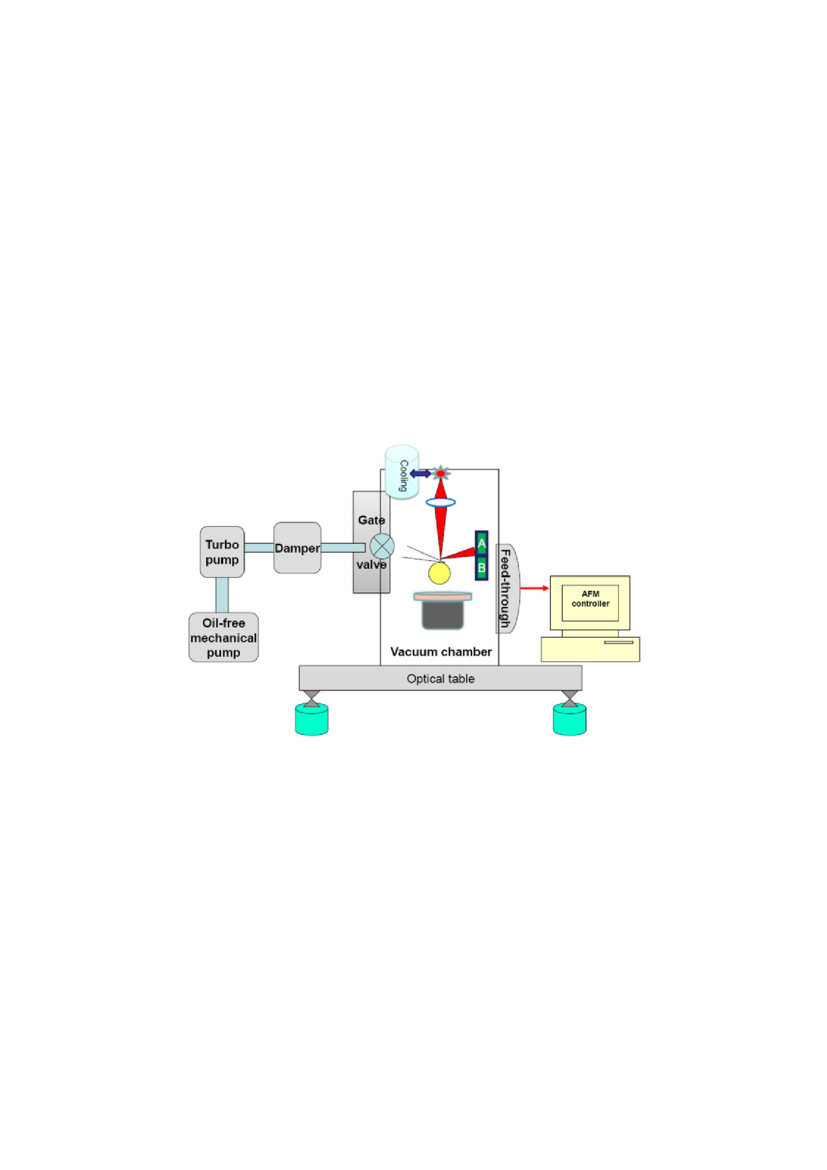
Figure 1: (Color online) Schematic of the experimental setup for measurement of the Casimir force using an AFM (see text for further discussion).

The commercial AFM (“Veeco”) used in our measurements was modified to be free of volatile organics. It was placed in a high vacuum chamber (see Fig. 1). Only oil-free mechanical and turbo pumps shown in Fig. 1 were used to obtain the vacuum. As a result, the experiments were done at a pressure of $10^{-6}\,$Torr. To ensure a low vibration noise environment, we used an optical table and a sand damper box to prevent coupling of the low frequency noise from the mechanical and turbo pumps (see Fig. 1).

After the first use40 of the AFM to measure the Casimir force, it has been employed for this purpose in many experiments.20 ; 21 ; 22 ; 23 ; 24 ; 25 ; 26 ; 27 ; 28 ; 41 ; 42 ; 43 ; 44 ; 45 The AFM system consists of a head, piezoelectric actuator, an AFM controller and computer. The head includes a diode laser which emits a collimated beam with a waist of tens of micrometers at the focus, an Au-coated cantilever with attached sphere that bends in response to the sphere-plate force, and photodetectors which measure the cantilever deflection through a differential measurement of the laser beam intensity. The plate is mounted on the top of the piezoelectric actuator which allows movement of the plate towards the sphere for a distance of $2\,\mu$m. To change the sphere-plate distance and avoid piezo drift and creep, a continuous 0.05 Hz triangular voltage signal was applied to this actuator. The application of the voltages to both the piezoelectric actuator and the laser, and the electronic processing and digitizing of the light collected by the photodetectors is done by the AFM controller (see Fig. 1). The computer is used for data acquisition. The cantilever deflection was recorded for about every 0.2 nm movement of the piezoelectric actuator.

More specifically, the scheme of the experiment is as follows. A total force $F_{\rm tot}$ acting between a sphere and a plate causes an elastic deflection $z$ of the cantilever in accordance with Hooke’s law

$$F_{\rm tot}=kz,$$ (1)

where $k$ is the spring constant. When the separation distance between the sphere and the plate is changed with the movement of the piezoelectric element, the cantilever deflection will correspond to the different forces it experiences at different separations. This deflection causes the deviation of the laser beam reflected off the cantilever tip which is measured with photodiodes A and B (see Fig. 1). The respective deflection signal $S_{\rm def}$ at various separation distances leads to a force-distance curve. Note that the signal $S_{\rm def}$ recorded by the photodetector is not in force units but has to be calibrated according to Eq. (1) and

$$z=mS_{\rm def},$$ (2)

where $m$ is the cantilever deflection in nm per unit photodetector signal (sometimes called the optical lever sensitivity). Here $S_{\rm def}$ is measured in volts and $m$ in nm/V.

To stabilize the laser used for the detection of deflection of the AFM cantilever, we employed a liquid nitrogen cooling system, which maintained the temperature of the AFM at 2^∘C. This is the temperature at which all measurements were performed in this experiment. We attached a copper braid to the surface of the AFM laser soarce. The other side of the braid was attached to a liquid nitrogen reservoir, which was also located inside the vacuum chamber. During the experiments the reservoir could be refilled through a liquid feed-through (see Fig. 1). The cooling system helped us to improve the spot size and to reduce the laser noise and drift. It also served as an additional cryo pump to obtain the high vacuum.

II.2 Sample preparation and characterization

The test bodies in this experiment consisted of an Au-coated sphere and quartz plate coated with an ITO film. Measurements of the Casimir force were performed for a sphere interacting with an untreated or, alternatively, an UV-treated ITO sample. First, we briefly consider the preparation of the sphere which was done similar to previous experiments.20 ; 21 ; 22 ; 27 ; 28 ; 40 ; 41 ; 44 ; 45

We used a polystyrene sphere which was glued with silver epoxy ($20\times 20\,\mu\mbox{m}^{2}$ spot) to the tip of a triangular silicon nitride cantilever with a nominal spring constant of order 0.01 N/m. The cantilever-sphere system was then coated with a 10 nm Cr layer followed by 20 nm Al layer and finally with a $105\pm 1\,$nm Au layer. This was done in an oil free thermal evaporator at a $10^{-7}\,$Torr vacuum. To make sure that the Au surface is sufficiently smooth, the coatings were performed at a very low deposition rate of 3.75 Å/min. The radius of an Au-coated sphere was determined using a scanning electron microscope to be $R=(101.2\pm 0.5)\,\mu$m. This was done after the end of force measurements.

The ITO film used in our experiment was prepared by RF sputtering (Thinfilm Inc.) on a 1 cm square single crystal quartz plate of 1 mm thickness. The film thickness and nominal resistivity were measured to be $d=(74.6\pm 0.2)\,$nm and $42\,\Omega$/sq, respectively. The surface of the ITO film was cleaned using the following procedure. First, the ITO sample was immersed in acetone and cleaned in an ultrasonic bath for 15 min. Then it was rinsed 3 times in DI water. This ultrasonic cleaning procedure and water rinsing was repeated next with methanol followed by ethanol. After completing of the ultrasonic cleaning, the sample was dried in a flow of pure nitrogen gas. Next, electrical contacts to copper wires were made by soldering with an indium wire. The ITO sample was now ready for force measurements in the high vacuum chamber which are done as described below.

After the force measurements were completed, the ITO sample was UV treated. For this purpose it was placed in a special air chamber containing a UV lamp. A pen-ray Mercury lamp with a length of $9.0^{\prime\prime}$ and outside diameter of $0.375^{\prime\prime}$ was used as the UV source. This lamp emits a spectrum with the primary peak at the wavelength 254 nm (5.4 mW/cm² at 1.9 cm distance) and a secondary peak at 365 nm (0.2 mW/cm² at 1.9 cm distance). During the UV treatment the sample was placed at 1 cm from the lamp for 12 hours. After finish of the UV treatment, the sample was cleaned as described above, and then the force measurements were again performed.

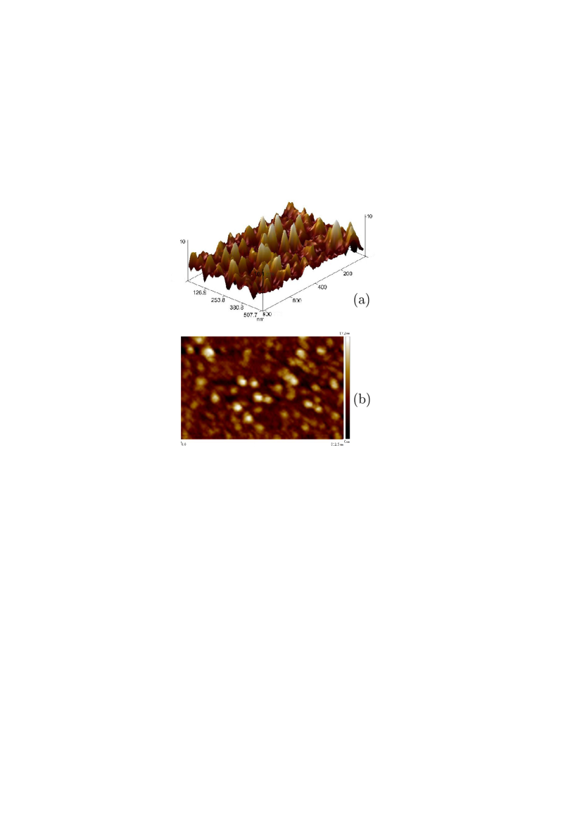
Figure 2: (Color online) (a) Typical three-dimensional AFM image of the surface of the ITO film. (b) Two-dimensional image of the same surface where lighter tone corresponds to larger height.

An important part of surface characterization is the measurement of roughness profiles on both an ITO sample and an Au-coated sphere. The roughness of the untreated and UV-treated ITO samples and the Au-coated sphere was investigated using the AFM. For the ITO plate before and after the UV treatment the roughness was found to be the same. A typical three-dimensional scan of an ITO plate is shown in Fig. 2(a). As can be seen in this figure, the roughness is represented by stochastically distributed distortions. For comparison purposes, the two-dimensional AFM scan of the surface of an ITO sample is shown in Fig. 2(b). Here, the lighter tone corresponds to the larger height above the minimum roughness level. The analysis of the data of AFM scans allows to determine the fraction of plate area $v_{i}^{\rm(ITO)}$ with heights $h_{i}^{\rm(ITO)}$ where $i=1,\,2,\,\ldots,\,N_{1}$ and $N_{1}$ is some chosen number. These heights are measured from the absolute minimum level on the test body $h_{1}^{\rm(ITO)}=0$. The resulting distribution function for an ITO plate is shown in Fig. 3(a). The zero roughness level on an ITO sample, relative to which the mean value of the roughness is equal to zero,6 ; 10 takes the value $H_{0}^{\rm(ITO)}=9.54\,$nm with $N_{1}=18$. The respective variance describing the stochastic roughness on an ITO sample6 ; 10 is given by $\delta_{\rm ITO}=2.28\,$nm. The distribution function for the roughness on an Au-coated sphere [$v_{i}^{\rm(Au)}$ as a function of $h_{i}^{\rm(Au)}$] is presented in Fig. 3(b). Here, the corresponding zero roughness level and variance are given by $H_{0}^{\rm(Au)}=11.51\,$nm and $\delta_{\rm Au}=3.17\,$nm, respectively, with $N_{2}=25$.

The presence of roughness on the surface determines the minimum separation distance that can be achieved when the test bodies are approaching. In fact the minimum separation $z_{0}$ (the so-called separation on contact) is the separation between the zero levels of the roughness on contact of the two surfaces. The actual absolute separation between the zero roughness levels on the bottom of an Au sphere and the ITO plate with account of Eq. (2) is given by

$$a=z_{0}+z_{\rm piezo}+mS_{\rm def},$$ (3)

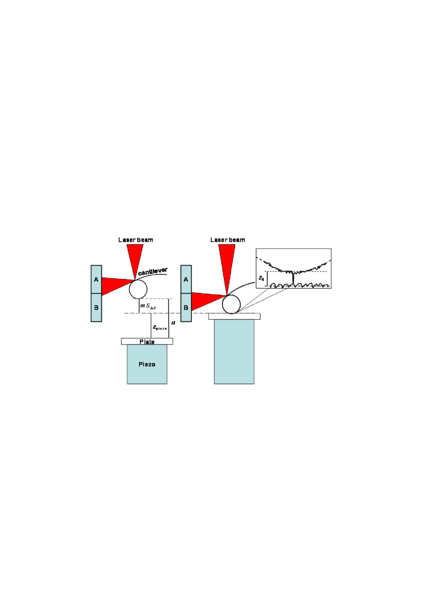
Figure 4: (Color online) Schematic explanation for the concept of the absolute separation distance $a$, and different contributions to it, i.e., distance traveled by the piezoelectric actuator $z_{\rm piezo}$, distance due to the deflection of the cantilever and separation on contact $z_{0}$.

where $z_{\rm piezo}$ is the distance moved by the plate owing to the voltage applied to the piezoelectric actuator. Figure 4 illustrates the meaning of the average separation on contact $z_{0}$ and other parameters entering Eq. (3). In Sec. VB the roughness profiles will be used to calculate the theoretical values of the Casimir force.

III Electrostatic calibrations

Electrostatic calibrations in the measurements of the Casimir force need extreme care. They allow determination with sufficient precision of values of such vital parameters as the residual potential difference $V_{0}$, the separation on contact $z_{0}$, the spring constant $k$, and the cantilever deflection coefficient $m$. During calibration process it is necessary to make sure that all relevant electric forces acting in the experimental configuration are included in the theoretical model used, and all possible background forces are negligibly small (see, for instance, a discussion46 ; 47 ; 48 ; 49 on the role of patch potentials which may exist due to the grain structure of metal coatings, surface contaminants etc.).

To make electrostatic measurements, the ITO plate was connected to a voltage supply (33120A,“Agilent Inc.”) operating with $1\,\mu$V resolution, while the sphere remained grounded. A 1 k$\Omega$ resistor was connected in series with the voltage supply to prevent surge currents and protect the sample surface during sphere-plate contact. The cantilever-sphere system was mounted on the AFM head which was connected to the ground. To reduce the electrical noise, care was taken to make Ohmic contacts and eliminate all Schottky barriers to the ITO plate and Au sphere. To minimize electrical ground loops, all the electrical ground connections were unified to the AFM ground. Ten different voltages $V_{i}$ ($i=1,\,2,\,\ldots,\,10$) were applied to the plate in each round of measurements. For an untreated plate these voltages were in the range from –260 to –110 mV in the first set of measurements and from –265 to –115 mV in the second set of measurements. For a UV-treated plate the applied voltages were from –25 to 150 mV and from –5 to 140 mV in the first and second set of measurements, respectively.

The total force between the sphere and the plate is given by the sum of electric $F_{\rm el}$ and Casimir $F$ forces. In accordance with Eqs. (1) and (2) it can be represented in the form

$$F_{\rm tot}(a,V_{i})=F_{\rm el}(a,V_{i})+F(a)=\tilde{k}S_{\rm def}(a,V_{i}),$$ (4)

where $\tilde{k}=km$ is the calibration constant. This force was measured as a function of separation. As described in Sec. IIA, to change the separation a continuous triangular voltage was applied to the AFM piezoelectric actuator. Note that this piezoelectric actuator was calibrated interferometrically.50 ; 51 Starting at the maximum separation of $2\,\mu$m, the ITO plate was moved towards the Au sphere and the corresponding cantilever deflection was recorded at every 0.2 nm until the plate contacted the sphere.

After the contact of the sphere and the plate, the cantilever-sphere system vibrated with a large amplitude. To allow time for this vibration to damp out, a 5 s delay was introduced after every cycle of data acquisation. To reduce random error, the total force at each of ten voltages applied to the untreated plate was measured ten times as a function of separation. The same was repeated for the UV-treated plate.

The electric force between a sphere and a plate made of conductors is given by6 ; 52

$$F_{\rm el}(a,V_{i})=X(a)(V_{i}-V_{0})^{2},$$ (5)

where

$$X(a)=2\pi\epsilon_{0}\sum_{n=1}^{\infty}\frac{\coth\alpha-n\coth{n\alpha}}{\sinh{n\alpha}},$$

$$\cosh\alpha=1+\frac{a}{R},$$ (6)

$V_{0}$ is the residual potential difference which can be present due to different work functions of the sphere and plate materials, and $\epsilon_{0}$ is the permittivity of the vacuum. In the wide range of separations the function $X(a)$ can be presented in the polynomial form21

$$X(a)=-2\pi\epsilon_{0}\sum_{i=-1}^{6}c_{i}\left(\frac{a}{R}\right)^{i}$$ (7)

with an error of about 0.01%. The coefficients $c_{i}$ in Eq. (7) are given by

$$c_{-1}=0.5,\ \ c_{0}=-1.18260,\ \ c_{1}=22.2375,$$

$$c_{2}=-571.366,\ \ c_{3}=9592.45,\ \ c_{4}=-90200.5,$$

$$c_{5}=383084,\ \ c_{6}=-300357.$$ (8)

As can be seen in Eqs. (4) and (5), the total force $F_{\rm tot}$ is characterized by the parabolic dependence of an applied voltage $V_{i}$. The same is true for the total deflection signal

$$S_{\rm def}(a,V_{i})=S(a)+\frac{X(a)}{\tilde{k}}(V_{i}-V_{0})^{2},$$ (9)

where $S(a)=F(a)/\tilde{k}$ is the deflection due to the Casimir force.

As an example, in Fig. 5 we present as squares the measured deflection signal $S_{\rm def}$ plotted as a function of the applied voltage for (a) the untreated and (b) UV-treated sample at a fixed separation $a=75\,$nm between the sphere and the plate. Then a $\chi^{2}$ fitting procedure was used to draw parabolas [the solid lines in Fig. 5(a,b)] and to determine their vertices and the coefficients $\beta(a)=X(a)/\tilde{k}$. This procedure was repeated at each separation distance with a step of 1 nm (though data were acquired about every 0.2 nm of $z_{\rm piezo}$, only interpolated values at 1 nm step were analyzed). The vertex of each parabola corresponds to $V_{0}$ at each respective separation. When $V_{i}=V_{0}$, the electrostatic force is equal to zero. The fitting procedure was also repeated at every separation $a$. From the parabolas shown in Fig. 5(a,b) it was obtained $V_{0}=-(195.9\pm 0.5)\,$mV and $V_{0}=(64.7\pm 0.4)\,$mV, respectively. The values of $V_{0}$ at separations from 60 to 300 nm are shown in Fig. 6(a) for an untreated and in Fig. 7(a) for a UV-treated sample in the first measurement set.

As can be seen in Figs. 6(a) and 7(a), there are anomalous dependences of $V_{0}$ on $a$, i.e., $V_{0}$ is not constant as expected if the electric force is described by the exact Eqs. (5) and (6). Such dependences were found in several experiments measuring the Casimir force and widely discussed in the literature.46 ; 47 ; 48 ; 49 ; 55 They are often interpreted as a manifectation of an additional electric force due to the presence of electrostatic surface impurities and space charge effects on the sphere or plate surfaces. In our case, however, these seeming anomalies do not indicate the presence of some extra electric force other than that given by Eqs. (5) and (6). The point is that the preceding analysis did not take into consideration the finiteness of the data acquisition rate and, more importantly, the mechanical drift of the sphere-plate separation. As a result, systematic deviations occurred in the residual potential difference $V_{0}$ in Figs. 6(a) and 7(a). These systematic deviations have been investigated,53 ; 54 and the respective corrections have been introduced in the data for $V_{0}$ as a function of $a$. The corrected results for $V_{0}$ as a function of separation for an untreated sample are shown in Fig. 6(b) and for a UV-treated sample in Fig. 7(b). Specifically, at $a=75\,$nm [see Fig. 5(a,b)] the corrected values of $V_{0}$ for an untreated and UV-treated samples are $V_{0}=-(195.6\pm 0.5)\,$mV and $V_{0}=(64.4\pm 0.4)\,$mV, respectively. As is seen in Figs. 6(b) and 7(b), after the proper corrections for the mechanical drift of separation distances and the finitness of the data acquisition rate are introduced, the residual potential difference remains constant in the limits of random errors. This excludes the presence of any perceptible electric force due to dust and contaminants in addition to the one given by Eqs. (5) and (6). From Figs. 6(b) and 7(b) the following mean values for the residual potential difference were found: $V_{0}=-(196.8\pm 1.5)\,$mV for the untreated sample and $V_{0}=(65\pm 2)\,$mV for the UV-treated sample.

We now discuss the deflection coefficient $m$ which enters Eq. (3) and, thus, is needed to determine both the absolute and relative sphere-plate separations. The deflection signals obtained by the application of the different voltages to the plate can be used to determine $m$. Here larger $(V-V_{0})^{2}$ will lead to correspondingly larger deflections and thus sphere-plate contact at smaller $z_{\rm piezo}$. This rate of change of contact point with $S_{\rm def}$ gives the value of $m$. However, as before, care must be taken to make a precise determination of the point of sphere-plate contact and correct the contact point for mechanical drift of the sphere-plate separation. Both corrections are already discussed in detail.53 ; 54 Briefly, the first of them is necessary, as even at the maximum acquisition rate, data points are widely separated near the point of contact due to the large force gradient at short separations. Thus an interpolation procedure has to be used to determine the exact contact point. With respect to the second correction, the contact points with two different applied $V$ but same $(V-V_{0})^{2}$ must be the same as the corresponding cantilever deflections are equal. Because of this any observed change in the contact point for these two applied voltages is due to sphere-plate drift. The drift rate is the time rate of change in the contact points for these voltages. Both corrections are needed to obtain the precise relative sphere-plate separation. As we discussed above, neglect of the drift correction leads to anomalous distance dependence behavior for the residual potential $V_{0}$. The corrected values of $m=(104.4\pm 0.5)\,$nm/V for the untreated sample and $m=(103.5\pm 0.6)\,$nm/V for the UV-treated sample were determined for the first measurement set.

In accordance with Eqs. (3) and (7), the parabola coefficient $\beta(a)$ depends on both the cantilever calibration constant $\tilde{k}$ and the average separation on contact $z_{0}$. Thus, the obtained values of $\beta(a)$ at different separations can be used to determine both $z_{0}$ and $\tilde{k}$ using the least $\chi^{2}$-fitting to Eq. (7) as described previously.53 ; 54 For this purpose the coefficient $\beta(a)$ was first fitted from a starting point of 60 nm to an end point $a_{\rm end}=1000\,$nm, and the values of $z_{0}$ and $\tilde{k}$ were determined. Then $a_{\rm end}$ was decreased to 900 nm and the fitting procedure repeated leading to the corresponding values of $z_{0}$ and $\tilde{k}$. The repetition of this procedure (in smaller steps below $a_{\rm end}=400\,$nm) results in Figs. 8(a) and 9(a) demonstrating the dependence of $z_{0}$ on $a_{\rm end}$ for an untreated and UV-treated samples, respectively, in the first set of our measurements. Similar results were obtained for $\tilde{k}$ as a function of $a_{\rm end}$.

As can be seen in Figs. 8(a) and 9(a), there is an anomalous dependence of $z_{0}$ on $a_{\rm end}$ caused, as above, by mechanical drift in the sphere-plate separation. After the respective corrections were introduced,53 ; 54 the obtained dependence of the separation on contact $z_{0}$ on $a_{\rm end}$ is shown in Fig. 8(b) for the untreated sample and in Fig. 9(b) for the UV-treated sample. It can be seen that in both cases the corrected values $z_{0}$ remain constant within the limits of random errors independently of the value of $a_{\rm end}$ chosen. The obtained mean values of $z_{0}$ are $z_{0}=(29.5\pm 0.4)\,$nm for the untreated sample and $z_{0}=(29.0\pm 0.6)\,$nm for the UV-treated sample. In Fig. 10(a,b) the corrected values of the calibration constant $\tilde{k}$ as a function of $a_{\rm end}$ obtained in the first measurement set are shown for an untreated and UV-treated samples, respectively. The respective mean values are as follows: $\tilde{k}=(1.45\pm 0.02)\,$nN/V and $\tilde{k}=(1.43\pm 0.02)\,$nN/V. As is seen in Fig. 10(a,b), the individual values of $\tilde{k}$ determined with different $a_{\rm end}$ are constant in the limits of random errors. This concludes the electrostatic calibration of our measurement system. It is pertinent to note that the fitting used above was made to only the well understood electric force in the sphere-plate configuration. In so doing it was confirmed that there are no other perceptible electric forces due to surface patches, contaminants, surface defects, such as pits and bubbles, etc.

The same calibration procedure, as described above, was repeated when performing the second set of our measurements. For the untreated sample, the following values of the parameters were found: $V_{0}=-(196.8\pm 1.5)\,$mV, $z_{0}=(29.6\pm 0.5)\,$nm, $\tilde{k}=(1.51\pm 0.02)\,$nN/V, and $m=(104.4\pm 0.5)\,$nm/V. For the UV-treated sample it was obtained: $V_{0}=(64.8\pm 2)\,$mV, $z_{0}=(29.0\pm 0.6)\,$nm, $\tilde{k}=(1.51\pm 0.02)\,$nN/V, and $m=(104.2\pm 0.6)\,$nm/V. The parameters presented in this section were used to convert the cantilever deflection signals into the values of the total force and to find the values of absolute separations.

Note that for all values of the above parameters the errors are indicated at a 95% confidence level.

IV Measurement results for the Casimir force and their errors

According to Eq. (4) the experimental results for the Casimir force between an Au sphere and an ITO plate are given by

$$F(a)=\tilde{k}S_{\rm def}(a,V_{i})-F_{\rm el}(a,V_{i}),$$ (10)

where the electric force $F_{\rm el}$ is expressed by Eqs. (5)–(7). At each separation $a$ the measurement of $S_{\rm def}$ with ten applied voltages was performed. This was repeated 10 times. Altogether, 100 values of the Casimir force at each separation were obtained from Eq. (10) in each measurement set for both untreated and UV-treated samples. Here, we present the main features of these data and determine the experimental errors.

IV.1 Mean measured Casimir forces

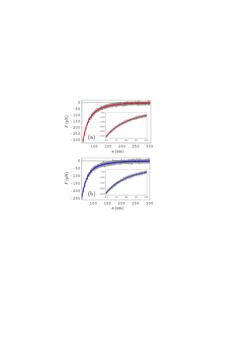
Figure 11: (Color online) Mean measured Casimir forces $F$ between the sphere and the plate as a function of separation $a$ are shown as solid lines for (a) the untreated and (b) UV-treated sample. In the inset the same is shown over a narrower range of separations. All 100 individual values of the measured force are shown as dots at separation distances at 5 nm intervals (1 nm intervals in the insets).

In Fig. 11 the mean measured Casimir forces obtained from one hundred individual values are shown as functions of separation with solid lines for (a) an untreated sample and (b) a UV-treated sample over the separation region from 60 to 300 nm in the first measurement set. In the insets, the same solid lines are reproduced over a more narrow separation region from 60 to 100 nm. As an illustration, Fig. 11 shows by dots all 100 individual values of the Casimir force plotted at separation distances with a step of 5 nm (in the insets with a step of 1 nm). Figure 11(a) indicates a 40%–50% decrease in the force magnitude in comparison with the case of two Au bodies in agreement with previous work23 ; 24 where a similar result was obtained for the Casimir pressure. For example at $a=80\,$nm the measured Casimir force is –144 pN in contrast to –269 pN for Au test bodies. As can be seen in Fig. 11(a,b), the magnitudes of the Casimir force from a UV-treated plate are 21% to 35% smaller than from an untreated plate.

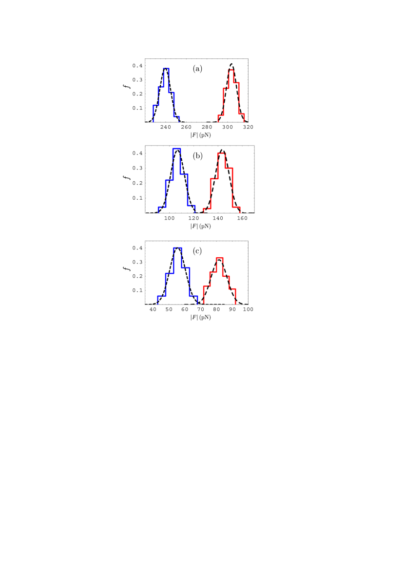
Figure 12: (Color online) The histograms for measured Casimir force $F$ for the untreated (right) and UV-treated (left) sample at separations (a) $a=60\,$nm, (b) $a=80\,$nm, and (c) $a=100\,$nm. $f$ is the fraction of 100 data points having the force values in the bin indicated by the vertical lines. The corresponding Gaussian distributions are shown by the dashed lines.

Figure 12 characterizes the statistical properties of the experimental data for an untreated (right) and UV-treated (left) samples by presenting the histograms for the measured Casimir force at separations (a) $a=60\,$nm, (b) $a=80\,$nm, and (c) $a=100\,$nm in the first measurement set. The histograms are described by Gaussian distributions (dashed lines) with the standard deviations equal to (a) $\sigma_{G}=4.6\,$pN (right), $\sigma_{G}=5.0\,$pN (left), (b) $\sigma_{G}=5.4\,$pN (right), $\sigma_{G}=5.4\,$pN (left), and (c) $\sigma_{G}=4.9\,$pN (right), $\sigma_{G}=4.7\,$pN (left). The values of the respective mean measured Casimir forces can be found in columns 2 and 5 of Table I. From Fig. 12 it is observed that the Gaussian distributions related to the untreated and UV-treated samples do not overlap lending great confidence to the effect of a decrease of the magnitude of the Casimir force under the influence of UV-treatment.

In Table I we present the mean magnitudes of the measured Casimir force at different separations (first column) ranging from 60 to 300 nm with the respective total experimental errors determined below in Sec. IVB. Columns 2 and 3 contain the force magnitudes obtained in the first and second measurement sets for the untreated sample, respectively. In columns 5 and 6 the respective results obtained for the UV-treated sample in the first and second measurement sets are presented. As can be seen in Table I, the measurement data obtained in the first and second measurement sets are in a very good agreement. All differences between them are much less than the total experimental errors presented in columns 4 and 7 (see Sec. IVB).

IV.2 Random, systematic and total experimental errors

Here we present the main results of the error analysis. The variance of the mean Casimir force calculated from 100 measurement results over the separation interval from 60 to 300 nm is shown as dots in Figs. 13(a) and 13(b) for the untreated and UV-treated samples, respectively. The respective mean values are separation independent: $\sigma=0.55\,$pN and $\sigma=0.5\,$pN. They are equal to the random errors in the measured Casimir force determined at a 67% confidence level. To determine the random error at a $\beta=95$% confidence level, one should multiply $\sigma$ by the student coefficient $t_{1.95/2}(99)=2$. Thus, the random errors at a 95% confidence level are equal to $\Delta^{\!r}F=1.1\,$pN and $\Delta^{\!r}F=1.0\,$pN, respectively.

According to Eq. (10), the systematic error in the measured Casimir forces is a combination of the systematic errors in the total measured force and subtracted electric force. The systematic error in the total measured force, $\Delta^{\!s}F_{\rm tot}$, is determined by the instrumental noise including the background noise level, and the errors in calibration. In Figs. 14(a) and 14(b) the error $\Delta^{\!s}F_{\rm tot}$ determined at a 95% confidence level is shown by the long-dashed lines as a function of separation for the untreated and UV-treated samples, respectively. The error in calculation of the electric force, which plays the role of a systematic error with respect to the Casimir force obtained from Eq. (10), is mostly determined by the errors in the measurement of separations. The latter are largely contributed by the errors in $z_{0}$ presented in Sec. III. As a result, for the first measurement set, the errors in absolute separations determined at a 95% confidence level are equal to $\Delta a=0.4\,$nm and $\Delta a=0.6\,$nm for the untreated and UV-treated samples, respectively. Note that due to Eq. (5) the error in $F_{\rm el}$ is different at different applied voltages $V_{i}$. As an illustration, Fig. 14(a,b) shows with short-dashed lines the mean $\Delta^{\!s}F_{\rm el}$ averaged over 10 applied voltages for the untreated and UV-treated samples, respectively. The respective solid lines in Figs. 14(a) and 14(b) demonstrate the total systematic errors $\Delta^{\!s}F$ in the Casimir force as a function of separation. They were obtained by adding in quadrature the systematic errors of the total and electric forces. As is seen in Fig. 14(a,b), at moderate and large separations the major contribution to the systematic error in the Casimir force is given by the systematic error in the total force. Only at short separations the error in the electric force contributes significantly to the systematic error in the Casimir force.

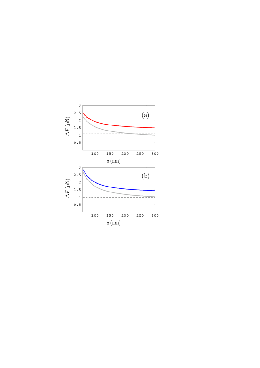
Figure 15: (Color online) The random $\Delta^{\!r}F$, systematic $\Delta^{\!s}F$, and total $\Delta^{\!\rm tot}F$ errors in the measured Casimir force determined at a 95% confidence level are shown as functions of separation $a$ by the dashed, lower solid and upper solid lines, respectively, for (a) the untreated and (b) UV-treated sample.

To obtain the total experimental error one should combine the random and systematic errors. In Fig. 15(a,b) the random errors are shown with the dashed lines for the untreated and UV-treated samples, respectively. The lower solid lines in the same figure represent the systematic errors which are dominant over the random ones in this experiment, especially at short separations. Keeping in mind that both the random and systematic errors considered above are characterized by the normal distribution, they should be added in quadrature. The resulting absolute total experimental errors $\Delta^{\!\rm tot}F$ determined at a 95% confidence level are shown by the upper solid lines for the untreated [Fig. 15(a)] and UV-treated [Fig. 15(b)] samples. The values of the absolute total experimental errors at different separations are presented in column 4 of Table I (for an untreated sample) and in column 7 for a UV-treated sample. The relative total experimental error in the measured Casimir force at $a=60\,$nm is equal to 0.82% and 1.2% for the untreated and UV-treated samples, respectively. With the increase of separation to $a=100\,$nm the respective errors increase to 2.3% and 3.6% and further increase to 13.4% and 24.2% when separation increases to $a=200\,$nm. At $a=300\,$nm the relative total experimental errors in the measured Casimir force for the untreated and UV-treated samples achieve 37.5% and 50%, respectively. For the sake of definiteness, these numerical values are given for the first measurement set. However, in both sets the total experimental errors are the same.

V Comparison between experiment and theory

We next discuss the comparison between the experimental data for the Casimir force and the theoretical predictions of the Lifshitz theory. We compute theoretical results using different approaches to the thermal Casimir force proposed in the literature.6 ; 8 ; 10 In the framework of the proximity force approximation which is clearly applicable57 for the parameters of this experiment the Lifshitz formula for the Casimir force between an Au-coated sphere and an ITO film deposited on a quartz plate takes the form

$$F(a,T) = k_{B}TR\sum_{l=0}^{\infty}{\vphantom{\sum}}^{\prime}\int_{0}^{\infty}k_{\bot}dk_{\bot}$$ (11)

$$\times \left\{\ln\left[1-r_{\rm TM}^{(1)}(i\xi_{l},k_{\bot})r_{\rm TM}^{(2)}(i\xi_{l},k_{\bot})\,e^{-2aq_{l}}\right]\right.$$

$$+\left.\ln\left[1-r_{\rm TE}^{(1)}(i\xi_{l},k_{\bot})r_{\rm TE}^{(2)}(i\xi_{l},k_{\bot})\,e^{-2aq_{l}}\right]\right\}.$$

Here, $k_{B}$ is the Boltzmann constant, $T=275\,$K, $\xi_{l}=2\pi k_{B}Tl/\hbar$ with $l=0,\,1,\,2,\,\ldots$ are the Matsubara frequencies, the primed sum means that the term with $l=0$ is divided by 2, $k_{\bot}$ is the projection of the wave vector onto the plate, and $q_{l}^{2}=k_{\bot}^{2}+\xi_{l}^{2}/c^{2}$. The reflection coefficients on an Au body modeled as a semispace for the transverse magnetic (TM) and transverse electric (TE) polarizations of the electromagnetic field are given by

$$r_{\rm TM}^{(1)}(i\xi_{l},k_{\bot})=\frac{\varepsilon_{l}^{(1)}q_{l}-k_{l}^{(1)}}{\varepsilon_{l}^{(1)}q_{l}+k_{l}^{(1)}},$$

$$r_{\rm TE}^{(1)}(i\xi_{l},k_{\bot})=\frac{q_{l}-k_{l}^{(1)}}{q_{l}+k_{l}^{(1)}},$$ (12)

where ${k_{l}^{(1)}}^{2}=k_{\bot}^{2}+\varepsilon_{l}^{(1)}\xi_{l}^{2}/c^{2}$ and $\varepsilon_{l}^{(1)}\equiv\varepsilon^{(1)}(i\xi_{l})$ is the dielectric permittivity of Au along the imaginary frequency axis.

The reflection coefficients of an ITO film deposited on quartz plate can be presented in the form6 ; 58

$$r_{\rm TM}^{(2)}(i\xi_{l},k_{\bot})=\frac{r_{\rm TM}^{(0,-1)}+r_{\rm TM}^{(-1,-2)}e^{-2k_{l}^{(-1)}d}}{1+r_{\rm TM}^{(0,-1)}r_{\rm TM}^{(-1,-2)}e^{-2k_{l}^{(-1)}d}}$$ (13)

and the same expression with the index TM replaced for TE. Here, $r_{\rm TM,TE}^{(n,n^{\prime})}$ are the reflection coefficients on an ITO layer of thickness $d$ ($n=0,{\ }n^{\prime}=-1$) and on a thick quartz plate modeled as a semispace ($n=-1,{\ }n^{\prime}=-2$)

$$r_{\rm TM}^{(n,n^{\prime})}(i\xi_{l},k_{\bot})=\frac{\varepsilon_{l}^{(n^{\prime})}k_{l}^{(n)}-\varepsilon_{l}^{(n)}k_{l}^{(n^{\prime})}}{\varepsilon_{l}^{(n^{\prime})}k_{l}^{(n)}+\varepsilon_{l}^{(n)}k_{l}^{(n^{\prime})}},$$

$$r_{\rm TE}^{(n,n^{\prime})}(i\xi_{l},k_{\bot})=\frac{k_{l}^{(n)}-k_{l}^{(n^{\prime})}}{k_{l}^{(n)}+k_{l}^{(n^{\prime})}}.$$ (14)

The notations used are the following: $\varepsilon_{l}^{(0)}=1$, $\varepsilon_{l}^{(-1)}=\varepsilon^{(-1)}(i\xi_{l})$ and $\varepsilon_{l}^{(-2)}=\varepsilon^{(-2)}(i\xi_{l})$ are the dielectric permittivities of ITO and quartz, respectively, and ${k_{l}^{(n)}}^{2}=k_{\bot}^{2}+\varepsilon_{l}^{(n)}\xi_{l}^{2}/c^{2}$. To perform computations of the Casimir force using Eqs. (11)–(14) one needs the dielectric permittivities of Au, ITO and quartz over a wide range of imaginary frequencies.

V.1 Complex indices of refraction and dielectric permittivities along imaginary frequencies

We describe the imaginary part of the dielectric permittivity of Au, ${\rm Im}\,\varepsilon^{(1)}(\omega)$, by means of the tabulated optical data.59 In the region $\omega<0.125\,$eV, where the optical data are missing, the extrapolation by means of the imaginary part of the Drude model dielectric permittivity with the plasma frequency $\omega_{p}=9.0\,$eV and relaxation parameter $\gamma=0.035\,$eV has been used. The dielectric permittivity of Au along the imaginary frequencies was obtained by means of the Kramers-Kronig relations.6 Using the so-called weighted Kramers-Kronig relations it was recently shown60 that the extrapolation by means of the Drude model with $\omega_{p}$ and $\gamma$ indicated above is in excellent agreement with the optical data measured over a wide frequency region.

For the underlying quartz plate we used the averaged dielectric permittivity obtained61 in the Ninham-Parsegian approximation5

$$\varepsilon^{(-2)}(i\xi_{l})=1+\frac{C_{\rm IR}}{1+\frac{\xi_{l}^{2}}{\omega_{\rm IR}^{2}}}+\frac{C_{\rm UV}}{1+\frac{\xi_{l}^{2}}{\omega_{\rm UV}^{2}}}$$ (15)

with the parameters $C_{\rm IR}=1.93$, $C_{\rm UV}=1.359$, $\omega_{\rm IR}=0.1378\,$eV, and $\omega_{\rm UV}=13.38\,$eV.

The dielectric permittivity of ITO strongly depends on a layer composition, thickness, etc. The literature on the subject is quite extensive.62 ; 63 ; 64 ; 65 ; 66 ; 67 ; 68 ; 69 Specifically, the parametrization of the dielectric permittivity of ITO was suggested69 using the Tauc-Lorentz model70 and the Drude model. This parametrization was used23 ; 24 for the comparison between the experimental data and computational results in the framework of the Lifshitz theory. It was found, however, that the computed magnitudes of the gradient of the Casimir force are substantially larger than the mean measured ones.

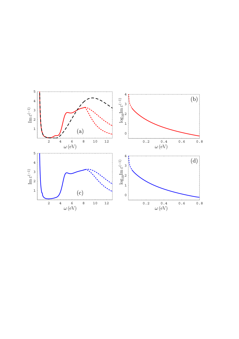
Figure 16: (Color online) The imaginary parts of dielectric permittivity of an ITO film ${\rm Im}\,\varepsilon^{(-1)}$ obtained from ellipsometry are shown as functions of frequency $\omega$ with the solid lines for (a,b) the untreated and (c,d) UV-treated sample in different frequency regions. The short-dashed lines (a,c) present possible extrapolations of the data to higher frequencies (see text for further discussion). The long-dashed line presents ${\rm Im}\,\varepsilon^{(-1)}$ from the paper by Fujiwara and Konde69 for the untreated ITO sample. The dashed lines (b,d) show the extrapolation to lower frequencies by means of the Drude model.

To characterize the dielectric properties of ITO films used in our experiment, we employed the untreated and UV-treated samples prepared in the same way and under the same conditions as those used in measurements of the Casimir force. The imaginary parts of the dielectric permittivity of ITO, ${\rm Im}\,\varepsilon^{(-1)}(\omega)$, was determined by means of ellipsometry (J. A. Woollam Co.71 ) for both untreated and UV-treated samples. In the frequency region from 0.04 to 0.73 eV the IR-VASE ellipsometer was used. The region of frequencies from 0.73 to 8.27 eV was covered with the help of VUV-VASE ellipsometer. The experimental data obtained from ellipsometric measurements were analyzed taking into account that the ITO resistivity decreases with depth. This results in different profiles of the dielectric permittivity of ITO at different depths and typically in the so-called top and bottom ${\rm Im}\,\varepsilon^{(-1)}(\omega)$ differing in the frequency range $\omega<0.4\,$eV. In Figs. 16(a,b) and 16(c,d) the experimental data for ${\rm Im}\,\varepsilon^{(-1)}(\omega)$ as a function of $\omega$ are shown by the solid lines for an untreated and UV-treated samples, respectively. In the frequency range shown in Fig. 16(a,c) the top and bottom permittivities coincide. The top ${\rm Im}\,\varepsilon^{(-1)}(\omega)$, which was found to lead to a good agreement with the measured Casimir forces for the untreated sample, is shown in Fig. 16(b,d) by the solid lines in the frequency region from 0.04 to 0.8 eV on a logarithmic scale. It was extrapolated in the region of low frequencies $\omega<0.04\,$eV by means of the imaginary part of the Drude dielectric function with the parameters $\omega_{p}=1.5\,$eV, $\gamma=0.128\,$eV and $\omega_{p}=1.5\,$eV, $\gamma=0.132\,$eV for an untreated and UV-treated samples, respectively (the dashed lines).

Precise computations of the Casimir force at separations $a\geq 60\,$nm require knowledge of dielectric properties up to $\omega\approx 16\,$eV. Because of this, the measured data for ${\rm Im}\,\varepsilon^{(-1)}(\omega)$ in Fig. 16(a,c) shown by the solid lines were extrapolated to higher frequencies by means of the imaginary part of an oscillator function

$${\rm Im}\,\varepsilon^{(-1)}(\omega)=\frac{g_{0}\gamma_{0}\omega}{(\omega^{2}-\omega_{0}^{2})^{2}+\gamma_{0}^{2}\omega^{2}}.$$ (16)

The reasonable smooth extrapolations are bounded between the short-dashed lines in Fig. 16(a,c). For an untreated sample [Fig. 16(a)] the upper short-dashed line is described by Eq. (16) with the oscillator parameters $g_{0}=240.54\,\mbox{eV}^{2}$, $\gamma_{0}=8.5\,$eV and $\omega_{0}=9.0\,$eV. For the lower short-dashed line we get $g_{0}=111.52\,\mbox{eV}^{2}$, $\gamma_{0}=4.0\,$eV and $\omega_{0}=8.0\,$eV. For the UV-treated sample [Fig. 16(c)] the oscillator parameters are $g_{0}=280.28\,\mbox{eV}^{2}$, $\gamma_{0}=9.2\,$eV and $\omega_{0}=9.8\,$eV and $g_{0}=128.28\,\mbox{eV}^{2}$, $\gamma_{0}=4.5\,$eV and $\omega_{0}=8.8\,$eV for the upper and lower short-dashed lines, respectively. As can be seen in Fig. 16(a,b,c,d), there are only minor differences in the imaginary parts of the dielectric permittivities for the untreated and UV-treated samples (the additional small peak near 3 eV for the untreated sample and insignificant variations in the oscillator structure). Note that the imaginary part of the ITO dielectric permittivity suggested earlier69 and used in computations of the gradient of the Casimir force23 ; 24 is shown by the long-dashed line in Fig. 16(a). It differs significantly from the dielectric permittivity of our untreated ITO sample. At lower frequencies deviations between the two permittivities increase due to the larger $\omega_{p}=1.94\,$eV used.69

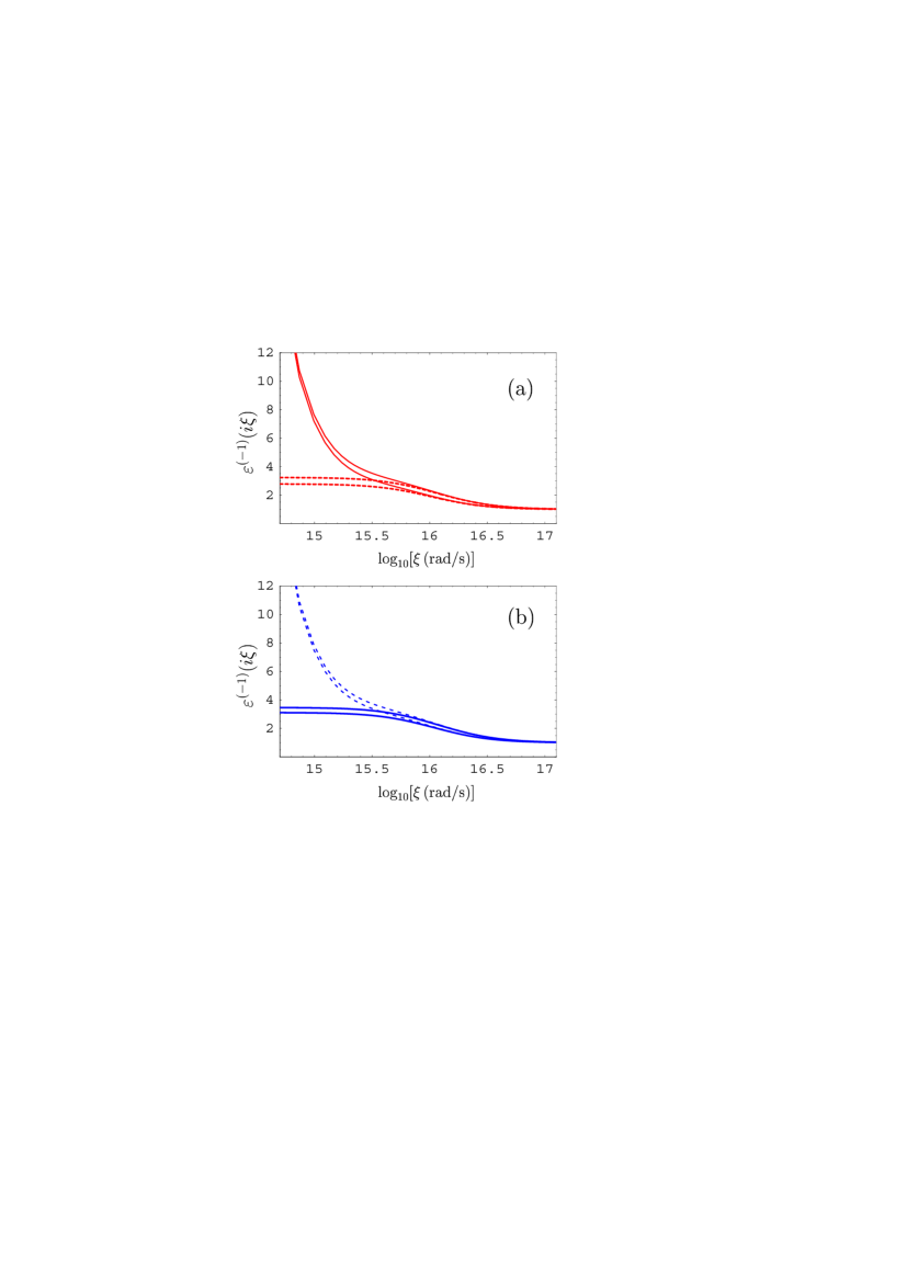
Figure 17: (Color online) The dielectric permittivity of an ITO film $\varepsilon^{(-1)}$ as a function of the imaginary frequency $i\xi$ for (a) the untreated and (b) UV-treated sample. The two solid and two dashed lines are obtained with different extrapolations of the ellipsometry data to higher frequencies [see Fig. 16(a,b)]. In Fig. 17(a) the solid and dashed lines correspond to included and omitted contribution of free charge carriers, respectively. In Fig. 17(b) the free charge carriers are included for the pair of dashed lines and omitted for the pair of solid lines.

Using the measured imaginary parts of dielectric permittivity of ITO in Fig. 16(a,b,c,d), the dielectric permittivities along the imaginary frequency axis were obtained by means of the Kramers-Kronig relation. The obtained results for the untreated sample are shown in Fig. 17(a) by the two solids lines corresponding to the two short-dashed lines in Fig. 16(a). In the same figure, the two dashed lines indicate the range of dielectric permittivities along the imaginary frequency axis for the case when the contribution of free charge carriers were disregarded. For the UV-treated sample the respective results obtained from the measured data in Fig. 16(c,d) by means of the Kramers-Kronig relation are shown in Fig. 17(b) by the two dashed lines. For the case when the charge carriers in the UV-treated sample are disregarded, the range of dielectric permittivities is indicated by the two solid lines. From the comparison of Fig. 17(a) with Fig. 17(b) it follows that the UV-treatment does not lead to any significant changes in dielectric permittivity of an ITO sample as a function of imaginary frequency.

V.2 Theoretical results using different approaches to the description of charge carriers

Using the dielectric permittivities discussed in Sec. VA we have calculated the Casimir force $F(a,T)$ from Eq. (11) acting between an Au-coated sphere and both untreated and UV-treated ITO samples over the range of separations from 60 to 300 nm. Then the surface roughness of Au and ITO films was taken into account by means of geometrical averaging.6 ; 10 Note that this approximate method leads to the same results as a more fundamental calculation based on the scattering approach72 at short separation distances where the roughness correction reaches maximum values (2.2% at $a=60\,$nm and less than 1% and 0.5% at $a\geq 90\,$nm and $a\geq 116\,$nm, respectively). At separations of about the correlation length of surface roughness the scattering approach predicts larger roughness corrections than the method of geometrical averaging. At such large separations, however, the effect of roughness is negligibly small and can be disregarded.6 As a result, the theoretical Casimir force between the rough surfaces of an Au sphere and ITO plate was computed according to the following expression:

$$F^{\rm theor}(a,T)=\sum_{i=1}^{N_{1}}\sum_{k=1}^{N_{2}}v_{i}^{\rm(ITO)}v_{k}^{\rm(Au)}$$

$$~{}~{}~{}~{}~{}~{}~{}~{}~{}~{}~{}~{}~{}~{}~{}~{}\times F(a+H_{0}^{\rm(ITO)}+H_{0}^{\rm(Au)}-h_{i}^{(\rm ITO)}-h_{k}^{(\rm Au)},T),$$ (17)

where all notations were introduced in Sec. IIB.

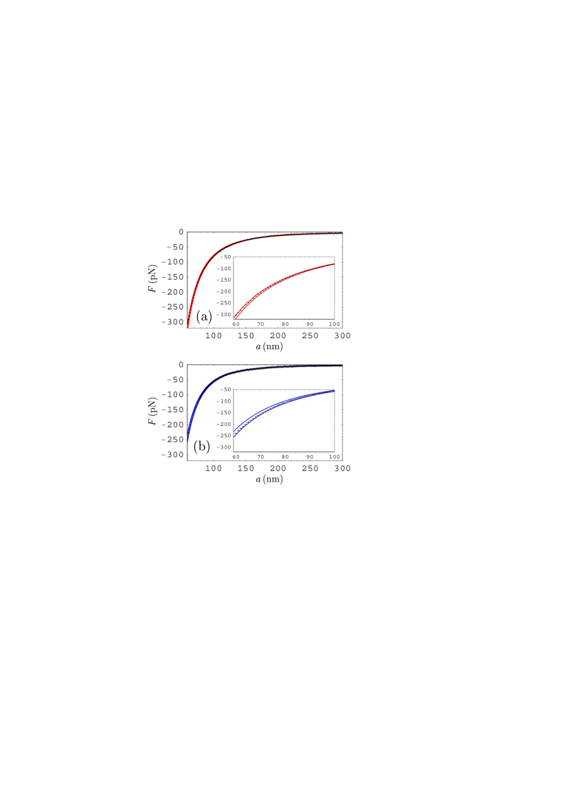
Figure 18: (Color online) The mean measured Casimir force $F$ indicated as crosses corresponding to error bars at 95% confidence level and the theoretical Casimir force $F^{\rm theor}$ shown by the pairs of solid lines as functions of separation $a$ for (a) the untreated sample (contribution of free charge carriers is included) and (b) UV-treated sample (contribution of free charge carriers is omitted). In the insets the same is shown over a narrower separation region from 60 to 100 nm.

The computational results using Eq. (17) in comparison with the experimental data are shown in Fig. 18(a,b). The theoretical Casimir forces between an Au sphere and an untreated ITO sample are shown by the two solid lines in Fig. 18(a) over the separation region from $a=60$ to 300 nm. In the inset the same lines over a more narrow separation region from 60 to 100 nm are presented. Computations were performed by Eqs. (11) and (17) with the dielectric permittivity of Au along the imaginary frequency axis indicated in Sec. VA and dielectric permittivity of an untreated ITO shown by the two solid lines in Fig. 17(a). In so doing the charge carriers of ITO were taken into account. The experimental data for the Casimir force (the first measurement set) are shown as crosses. The arms of the crosses indicate the total experimental errors in the separation distances and forces determined at a 95% confidence level (see Sec. IVB). As can be seen in Fig. 18(a), the experimental data are in a very good agreement with the theory within the limits of theoretical uncertainties shown by the band between the two solid lines.

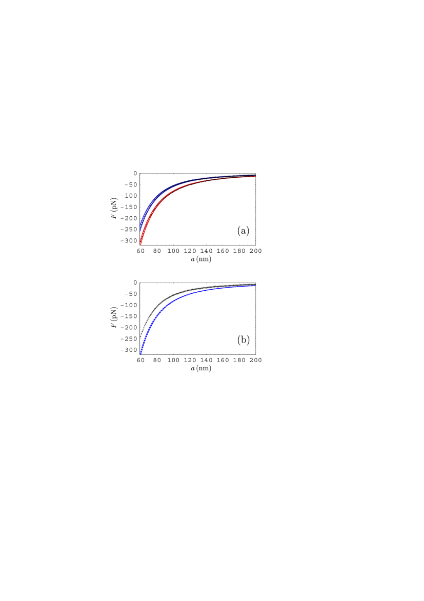
Figure 19: (Color online) (a) The mean measured Casimir force $F$ as a function of separation $a$ is indicated as upper and lower sets of crosses corresponding to error bars at 95% confidence level for the UV-treated and untreated samples, respectively. The respective upper and lower pairs of the solid lines show the theoretical results computed with omitted and included contribution of free charge carriers. (b) The mean measured Casimir force $F$ as a function of separation $a$ for a UV-treated sample is indicated as crosses corresponding to error bars at 95% confidence level. The two dashed lines show the theoretical results $F^{\rm theor}$ computed with the contribution of free charge carriers included for the UV-treated sample.

In Fig. 18(b) the comparison between the theoretical results (the band between the two solid lines) and the experimental data (crosses) is presented for a UV-treated sample. Here, to achieve the agreement between experiment and theory, the charge carriers in the ITO sample were disregarded. This means that the dielectric permittivity of the UV-treated ITO shown by the two solid lines in Fig. 17(b) has been used in computations. The inset in Fig. 18(b) demonstrates the agreement achieved over a narrower separation region from 60 to 100 nm. The use of the dielectric permittivity of an ITO film with the contribution of charge carriers disregarded may seem somewhat unjustified because the electric properties of an untreated and a UV-treated ITO samples are very close. To analyze this problem in more detail, in Fig. 19(a) we present the comparison between experiment and theory for an untreated (the lower pair of solid lines) and a UV-treated (the upper pair of solid lines) samples over a separation range from 60 to 200 nm. As above, the experimental data are shown as crosses. The same dielectric permittivities as in Fig. 18(a,b) were used in computations. From Fig. 19(a) it is observed that theoretical results with included (the lower pair of solid lines) and disregarded (the upper pair of solid lines) contribution of charge carriers do not overlap and are in very good agreement with the measurement data for respective ITO samples.

Furthermore, in Fig. 19(b) we plot as crosses the measured Casimir forces between a sphere and a UV-treated sample. In the same figure, the two dotted lines show the computational results by using the seemingly most natural dielectric permittivity of a UV-treated sample shown by the two dashed lines in Fig. 17(b), i.e., taking into account the free charge carriers. As can be observed in Fig. 19(b), substitution of actual dielectric properties of a UV-treated ITO film at room temperature in the Lifshitz theory results in drastic contradiction with the measured Casimir forces. Note that the use of the bottom dielectric permittivity of an ITO film discussed above instead of the top would lead to larger in magnitude Casimir forces, i.e., to further increasing disagreement between experiment and theory (note that the difference between the bottom and top permittivities is relevant only to the contribution of free charge carriers).

In order to appreciate why the Lifshitz theory with the dielectric permittivity disregarding charge carriers leads to agreement with the measurement data for the UV-treated sample, we consider the phenomenological prescription6 ; 10 formulated earlier to account for the results of several experiments27 ; 28 ; 29 ; 30 ; 35 ; 36 discussed in Sec. I. According to this prescription, for dielectrics and semiconductors of dielectric type free charge carriers should be disregarded, whereas for metals they should be taken into account by means of the plasma model. An important point in support of this prescription is that the inclusion of relaxation properties of electrons for metals with perfect crystal lattices and dc conductivity for dielectrics in the Lifshitz theory results in violation of the Nernst heat theorem.6 ; 10 The phenomenological prescription6 ; 10 gave rise to controversial discussions in the literature and even to attempts to modify the Lifshitz theory.6 ; 10 One interesting consequence of this prescription is the possibility to obtain significantly different Casimir forces from samples with nearly equal dielectric permittivities. To do this, one should consider a patterned Si plate with two sections of different doping concentrations which oscillates in the horizontal direction below an Au sphere.37 If doping concentrations are chosen only slightly below and above the critical value, the halves of a Si plate will be in dielectric and metallic states, respectively. This would lead to significantly different Casimir forces with almost equal dielectric permittivities along the imaginary frequency axis.

At this point one can hypothesize that the UV treatment of the plate results in the Mott-Anderson phase transition of an ITO film to a dielectric state without noticeable change of its optical properties at room temperature. This hypothesis is supported by the observation that the UV treatment of ITO leads to a lower mobility of charge carriers.73 The hypothesis proposed could be verified in future by the investigation of electrical properties of the UV-treated ITO films at very low temperature. Specifically, if the UV treatment transforms the ITO film from metallic to dielectric state, the electric conductivity (which is similar for an untreated and UV-treated films at room temperature) should vanish when the temperature vanishes.

In the above computations the low-frequency behavior of the dielectric permittivities of both Au and an untreated ITO was described by the Drude model. We emphasize that almost the same computational results leading to the same measure of agreement between experiment and theory are obtained when the free charge carriers in Au are described by the plasma model with the plasma frequency $\omega_{p}=9.0\,$eV. The same is correct for untreated ITO, but in this case the charge carriers should be described by the plasma model with the so-called longitudinal 63 $\omega_{p}=1.3\,$eV. The value of this parameter is determined by the physical processes at high frequencies rather than from the extrapolation of the optical data measured at low frequencies to zero frequency. Note that the use of the plasma model for the description of charge carriers for the UV-treated sample leads to the same computational results for the Casimir force as shown by the two dashed lines in Fig. 19(b). Thus, the inclusion of charge carriers into the Lifshitz theory for the UV-treated sample cannot be reconciled with the experimental data for the Casimir force shown in Fig. 19(b) as crosses.

In this section the comparison between experiment end theory was made using the data from the first measurement set. The experimental data from the second set (see Table I) were also compared with the same theoretical approaches. The results obtained are found indistinguishable from those presented in Figs. 18(a,b) and 19(a,b). Because of this, we do not discuss them at greater length.

VI Conclusions and discussion

In the foregoing we have described the experimental observation of the effect of significant decrease in the magnitude of the Casimir force between an Au sphere and an ITO plate after the UV-treatment of the latter. The main and unexpected feature of the observed phenomenon is that a decrease in force from 21% to 35% depending on separation distance between the sphere and the plate was achieved with no significant change of the dielectric permittivity of the ITO film under the UV-treatment.

Measurement of the Casimir force requires precision laboratory techniques and extreme care in all preparation procedures and analysis. We performed our measurements using a multimode AFM in a high vacuum chamber. In Sec. II we have described the setup used and all stages of the sample preparation and characterization including the procedure of UV-treatment.

Special attention was paid to electrostatic calibrations which are described in Sec. III. In the last few years calibration of the Casimir force measurement setup has attracted considerable interest and even become controversial.46 ; 47 ; 48 ; 49 ; 55 It was claimed that anomalous dependences of the residual potential difference and separation on contact on the separation distance observed in several experiments cast doubts on the measurements of the Casimir force performed to date. It was also suggested that inasmuch electrostatic calibrations are based on a fitting procedure there is no principal difference detween independent measurements of the Casimir force20 ; 21 ; 22 ; 23 ; 24 ; 25 ; 26 ; 27 ; 28 ; 29 ; 30 ; 35 ; 36 ; 37 ; 38 ; 40 ; 41 ; 42 ; 43 ; 44 ; 45 and deriving the Casimir force by means of a fit from some much larger measured force of hypothetical origin.31 In this respect we would like to note that the calibration consists in determination of the parameters of a setup using well established physical laws (in our case of electrostatics) and involves only well understood and precisely measured forces. Because of this, the use of some fitting procedure in the process of calibration is not, under any circumstances, to be regarded as an evidence in favor of the statement that the measurement of the Casimir force is not independent. In fact, the calibration procedure is a part of any measurement. On the contrary, the extraction of the Casimir force by means of the fitting procedure from much larger force, of which the major contribution is not measured and whose origin is not clearly understood,31 indicates that this is not an independent measurement.

Keeping in mind these complicated issues, in Sec. III we have analyzed in detail different systematic deviations arising in the calibration process. These systematic deviations are some biases in a measurement which always make the measured value higher or lower than the true value. We demonstrated that if such deviations are not taken into account and properly addressed, this results in the anomalies described in the literature. To the contrary, we have shown that if the systematic deviations due to finiteness of the acquisition rate and drift of sphere-plate separation are measured and removed by means of introducing the respective corrections, one arrives at the situation with no anomalies in accordance with the well established laws of electrostatics.

In Sec. IV we have presented our measurement results and the analysis of random, systematic and total experimental errors. Here the main result of our paper is demonstrated, i.e., that the UV-treatment of an ITO film results in significant decrease in the magnitude of the Casimir force. The histograms presented confirm that the Gaussian distributions of the Casimir force between an Au sphere and an untreated and, alternatively, a UV-treated sample do not overlap giving a strong confirmation of the effect observed. The values of the total experimental errors determined at a 95% confidence level bring the final confirmation to the effect of a decrease in the magnitude of the Casimir force under UV treatment of the ITO sample.

The comparison of the experimental results obtained with the Lifshitz theory was performed in Sec. V. While the experimental data for an untreated sample are in a very good agreement with conventional applications of the Lifshitz formula for metals (i.e., with inclusion of free charge carrier contribution), the comparison of the data with theory for the UV-treated sample resulted in a puzzle. The measured data were found to be in a very good agreement with computations if the contribution of free charge carriers is disregarded. In contrast, the inclusion of the contribution of free charge carriers to the dielectric permittivity of the UV-treated ITO sample resulted in complete disagreement between the data and the computational results. This is really puzzling if we take into consideration that the ellipsometry measurements performed for both the untreated and UV-treated ITO films did not reveal any significant differences in the imaginary parts of their dielectric permittivities. According to the hypothetical explanation of this phenomenon proposed in Sec. V, the UV treatment of the ITO film resulted in its Mott-Anderson phase transition from the metal to dielectric state with no significant changes in optical and electrical properties at room temperature. Further investigations are needed for the confirmation or rejection of this hypothesis. Specifically, one should investigate the physical properties of complicated physical compounds including their interaction with zero-point and thermal fluctuations of the electromagnetic field.

Whether the proposed theoretical explanation is correct or not, the observed phenomenon of the decreased Casimir force after the UV treatment of an ITO sample can find prospective applications in nanotechnology. In comparison with the case of an Au sphere interacting with an Au plate, the Casimir force between an Au sphere and a UV-treated ITO plate is decreased up to 65%. This result is of much practical importance for problems of lubrication and stiction in micro- and nanoelectromechanical systems where the Casimir and van der Waals forces may lead to collapse of the moving parts of devices to the fixed electrodes, i.e., to loss of functionality in devices. Significant decrease in the magnitude of the Casimir force should be helpful for the resolution of such problems.

         

         

         

Figure 3: The fractions of the area $v_{i}$ covered with roughness of heights $h_{i}$ for (a) ITO and (b) Au surfaces.

         

         

Figure 5: The deflection signal $S_{\rm def}$ as a function of the applied voltage $V$ for (a) the untreated and (b) UV-treated sample at a fixed separation $a=75\,$nm between the sphere and the plate.

         

Figure 6: The residual potential difference $V_{0}$ between the sphere and the plate surfaces as a function of separation $a$ for the untreated sample (a) with no corrections for systematic deviations due to drift and finite data acquisition rate and (b) with corrections of same deviations.

         

Figure 7: The residual potential difference $V_{0}$ between the sphere and the plate surfaces as a function of separation $a$ for the UV-treated sample (a) with no corrections for systematic deviations due to drift and finite data acquisition rate and (b) with corrections of same deviations.

         

Figure 8: The separation on contact $z_{0}$ between the sphere and the plate surfaces as a function of the end point $a_{\rm end}$ for the untreated sample (a) with no corrections for systematic deviations due to drift and finite data acquisition rate and (b) with corrections of same deviations.

         

Figure 9: The separation on contact $z_{0}$ between the sphere and the plate surfaces as a function of the end point $a_{\rm end}$ for the UV-treated sample (a) with no corrections for systematic deviations due to drift and finite data acquisition rate and (b) with corrections of same deviations.

         

Figure 10: The calibration constant $\tilde{k}$ as a function of the end point $a_{\rm end}$ with corrections for systematic deviations introduced for (a) the untreated sample and (b) UV-treated sample.

         

         

         

Figure 13: The variance $\sigma$ of the mean Casimir force calculated from 100 measurement results as a function of separation $a$ for (a) the untreated and (b) UV-treated sample.

         

Figure 14: The systematic error in the total measured force $\Delta^{\!s}F_{\rm tot}$, the mean systematic error in the electric force $\Delta^{\!s}F_{\rm el}$ averaged over 10 applied voltages, and the systematic error in the Casimir force $\Delta^{\!s}F$ as a function of separation $a$ are shown by the long-dashed lines, short-dashed lines, and solid lines, respectively, for (a) the untreated and (b) UV-treated sample.

         

         

         

         

         

Table 1: The magnitudes of the mean measured Casimir forces between an Au sphere and an ITO plate at different separations (column 1) for the untreated (columns 2 and 3 for the two measurement sets) and UV-treated (columns 5 and 6 for the two measurement sets) samples. Columns 4 and 7 contain the total experimental errors determined at a 95% confidence level for the untreated and UV-treated sample, respectively.

$a$	$|F|$(pN), untreated sample			$|F|$(pN), UV-treated sample
(nm)	1st set	2nd set	$\Delta^{\!\rm tot}F$	1st set	2nd set	$\Delta^{\!\rm tot}F$
60	303.8	304.4	2.5	239.5	238.8	2.9
70	204.4	204.0	2.3	156.4	155.6	2.5
80	143.6	143.7	2.1	106.7	105.5	2.3
90	107.0	106.2	2.0	75.4	74.6	2.1
100	81.6	80.7	1.9	55.5	54.9	2.0
120	50.1	51.1	1.8	33.0	32.9	1.8
140	32.9	33.4	1.7	22.6	21.2	1.7
160	21.8	23.3	1.7	15.4	15.1	1.6
180	16.3	15.3	1.6	10.5	10.9	1.6
200	11.9	11.0	1.6	6.6	8.0	1.6
220	6.7	7.6	1.6	5.5	6.3	1.5
240	5.8	5.5	1.5	4.4	4.2	1.5
260	5.7	5.3	1.5	3.7	3.8	1.5
280	4.6	4.2	1.5	3.1	3.2	1.5
300	4.0	4.1	1.5	3.0	2.4	1.5

References

- (1) P. W. Milonni, The Quantum Vacuum (Academic Press, San Diego, 1994).
- (2) M. Krech, The Casimir Effect in Critical Systems (World Scientific, Singapore, 1994).
- (3) V. M. Mostepanenko and N. N. Trunov, The Casimir Effect and its Applications (Clarendon, Oxford, 1997).
- (4) K. A. Milton, The Casimir Effect (World Scientific, Singapore, 2001).
- (5) V. A. Parsegian, Van der Waals Forces: A Handbook for Biologists, Chemists, Engineers, and Physicists (Cambridge University Press, Cambridge, 2005).
- (6) M. Bordag, G. L. Klimchitskaya, U. Mohideen, and V. M. Mostepanenko, Advances in the Casimir Effect (Oxford University Press, Oxford, 2009).
- (7) M. Bordag, U. Mohideen, and V. M. Mostepanenko, Phys. Rep. 353, 1 (2001).
- (8) K. A. Milton, J. Phys. A: Math. Gen. 37, R209 (2004).
- (9) S. K. Lamoreaux, Rep. Progr. Phys. 68, 201 (2005).
- (10) G. L. Klimchitskaya, U. Mohideen, and V. M. Mostepanenko, Rev. Mod. Phys. 81, 1827 (2009).
- (11) G. L. Klimchitskaya, U. Mohideen, and V. M. Mostepanenko, Int. J. Mod. Phys. B 25, 171 (2011).
- (12) A. W. Rodriguez, F. Capasso, and S. G. Johnson, Nature Photon. 5, 211 (2011).
- (13) H. B. G. Casimir, Proc. K. Ned. Akad. Wet. B 51, 793 (1948).
- (14) H. B. G. Casimir and D. Polder, Phys. Rev. 73, 360 (1948).
- (15) H. B. Chan, V. A. Aksyuk, R. N. Kleiman, D. J. Bishop, and F. Capasso, Science 291, 1941 (2001).
- (16) H. B. Chan, V. A. Aksyuk, R. N. Kleiman, D. J. Bishop, and F. Capasso, Phys. Rev. Lett. 87, 211801 (2001).
- (17) E. Buks and M. L. Roukes, Phys. Rev. B 63, 033402 (2001).
- (18) E. Buks and M. L. Roukes, Europhys. Lett. 54, 220 (2001).
- (19) E. M. Lifshitz, Zh. Eksp. Teor. Fiz. 29, 94 (1956) [Sov. Phys. JETP 2, 73 (1956)].
- (20) F. Chen, U. Mohideen, G. L. Klimchitskaya, and V. M. Mostepanenko, Phys. Rev. A 72, 020101(R) (2005).
- (21) F. Chen, U. Mohideen, G. L. Klimchitskaya, and V. M. Mostepanenko, Phys. Rev. A 74, 022103 (2006).
- (22) F. Chen, G. L. Klimchitskaya, V. M. Mostepanenko, and U. Mohideen, Phys. Rev. Lett. 97, 170402 (2006).
- (23) S. de Man, K. Heeck, R. J. Wijngaarden, and D. Iannuzzi, Phys. Rev. Lett. 103, 040402 (2009).
- (24) S. de Man, K. Heeck and D. Iannuzzi, Phys. Rev. A 82, 062512 (2010).
- (25) G. Torricelli, P. J. van Zwol, O. Shpak, C. Binns, G. Palasantzas, B. J. Kooi, V. B. Svetovoy, and M. Wuttig, Phys. Rev. A 82, 010101(R) (2010).
- (26) G. Torricelli, I. Pirozhenko, S. Thornton, A. Lambrecht, and C. Binns, Europhys. Lett. 93, 51001 (2011).
- (27) F. Chen, G. L. Klimchitskaya, V. M. Mostepanenko, and U. Mohideen, Optics Express 15, 4823 (2007).
- (28) F. Chen, G. L. Klimchitskaya, V. M. Mostepanenko, and U. Mohideen, Phys. Rev. B 76, 035338 (2007).
- (29) R. S. Decca, D. López, E. Fischbach, G. L. Klimchitskaya, D. E. Krause, and V. M. Mostepanenko, Phys. Rev. D 75, 077101 (2007).
- (30) R. S. Decca, D. López, E. Fischbach, G. L. Klimchitskaya, D. E. Krause, and V. M. Mostepanenko, Eur. Phys. J. C 51, 963 (2007).
- (31) A. O. Sushkov, W. J. Kim, D. A. R. Dalvit, and S. K. Lamoreaux, Nature Phys. 7, 230 (2001).
- (32) M. Masuda and M. Sasaki, Phys. Rev. Lett. 102, 171101 (2009).
- (33) V. B. Bezerra, G. L. Klimchitskaya, U. Mohideen, V. M. Mostepanenko, and C. Romero, Phys. Rev. B 83, 075417 (2011).
- (34) G. L. Klimchitskaya, M. Bordag, E. Fischbach, D. E. Krause, and V. M. Mostepanenko, Int. J. Mod. Phys. A 26, 3918 (2011).
- (35) J. M. Obrecht, R. J. Wild, M. Antezza, L. P. Pitaevskii, S. Stringari, and E. A. Cornell, Phys. Rev. Lett. 98, 063201 (2007).
- (36) G. L. Klimchitskaya and V. M. Mostepanenko, J. Phys. A: Math. Theor. 41, 312002(F) (2008).
- (37) C.-C. Chang, A. A. Banishev, G. L. Klimchitskaya, V. M. Mostepanenko, and U. Mohideen, Phys. Rev. Lett. 107, 090403 (2011).
- (38) V. B. Bezerra, G. L. Klimchitskaya, and V. M. Mostepanenko, Phys. Rev. A 66, 062112 (2002).
- (39) U. Mohideen and A. Roy, Phys. Rev. Lett. 81, 4549 (1998).
- (40) B. W. Harris, F. Chen, and U. Mohideen, Phys. Rev. A 62, 052109 (2000).
- (41) G. Jourdan. A. Lambrecht, F. Comin, and J. Chevrier, Europhys. Lett. 85, 31001 (2009).
- (42) P. J. van Zwol, V. B. Svetovoy, and G. Palasantzas, Phys. Rev. B 80, 235401 (2009).
- (43) H.-C. Chiu, G. L. Klimchitskaya, V. N. Marachevsky, V. M. Mostepanenko, and U. Mohideen, Phys. Rev. B 80, 121402(R) (2009).
- (44) H.-C. Chiu, G. L. Klimchitskaya, V. N. Marachevsky, V. M. Mostepanenko, and U. Mohideen, Phys. Rev. B 81, 115417 (2010).
- (45) W. J. Kim, M. Brown-Hayes, D. A. R. Dalvit, J. H. Brownell, and R. Onofrio, Phys. Rev. A 78, 020101(R) (2008).
- (46) R. S. Decca, E. Fischbach, G. L. Klimchitskaya, D. E. Krause, D. López, U. Mohideen, and V. M. Mostepanenko, Phys. Rev. A 79, 026101 (2009).
- (47) W. J. Kim, M. Brown-Hayes, D. A. R. Dalvit, J. H. Brownell, and R. Onofrio, Phys. Rev. A 79, 026102 (2009).
- (48) R. S. Decca, E. Fischbach, G. L. Klimchitskaya, D. E. Krause, D. López, U. Mohideen, and V. M. Mostepanenko, Int. J. Mod. Phys. A 26, 3930 (2011).
- (49) F. Chen and U. Mohideen, Rev. Sci. Instrum. 72, 3100 (2001).
- (50) H. E. Grecco and O. E. Martinez, Appl. Opt. 41, 6646 (2002).
- (51) W. R. Smythe, Electrostatics and Electrodynamics (McGraw-Hill, New York, 1950).
- (52) W. J. Kim, M. Brown-Hayes, D. A. R. Dalvit, J. H. Brownell, and R. Onofrio, J. Phys.: Conf. Ser. 161, 012004 (2009).
- (53) H.-C. Chiu, C.-C. Chang, R. Castillo-Garza, F. Chen, and U. Mohideen, J. Phys. A 41, 164022 (2008).
- (54) A. A. Banishev, C.-C. Chang, and U. Mohideen, Int. J. Mod. Phys. A 26, 3900 (2011).
- (55) B. Geyer, G. L. Klimchitskaya, and V. M. Mostepanenko, Phys. Rev. A 82, 032513 (2010).
- (56) M. S. Tomaš, Phys. Rev. A 66, 052103 (2002).
- (57) Handbook of Optical Constants of Solids, ed. E. D. Palik (Academic, New York, 1985).
- (58) G. Bimonte, Phys. Rev. A 83, 042109 (2011).
- (59) L. Bergström, Adv. Coll. Interface Sci. 70, 125 (1997).
- (60) I. Hamberg, C. G. Granqvist, K.-F. Bergren, B. E. Sernelius, and L. Engström, Vacuum 35, 207 (1985).
- (61) I. Hamberg and C. G. Granqvist, J. Appl. Phys. 60, R123 (1986).
- (62) S. H. Brewer and S. Franzen, J. Phys. Chem. B 106, 12986 (2002).
- (63) P. K. Biswas, A. De, N. C. Pramanik, P. K. Chakraborty, K. Ortner, V. Hock, and S. Korder, Mater. Lett. 57, 2326 (2003).
- (64) J. Ederth, P. Johnsson, G. A. Niklasson, A. Hoel, A. Hultåker, P. Heszler, and C. G. Granqvist, Phys. Rev. B 68, 155410 (2003).
- (65) F. Matino, L. Persano, V. Arima, D. Pisignano, R. I. R. Blyth, R. Cingolani, and R. Rinaldi, Phys. Rev. B 72, 085437 (2005).
- (66) S. H. Brewer, D. Wicaksana, J.-P. Maria, A. I. Kingon, and S. Franzen, Chem. Phys. 313, 25 (2005).
- (67) H. Fujiwara and M. Kondo, Phys. Rev. B 71, 075109 (2005).
- (68) G. E. Jellison, Jr. and F. A. Modine, Appl. Phys. Lett. 69, 371 (1996).
- (69) http://www.jawoollam.com
- (70) P. A. Maia Neto, A. Lambrecht, and S. Reynaud, Phys. Rev. A 72, 012115 (2005).
- (71) R. Castillo-Garza, C.-C. Chang, D. Jimenez, G. L. Klimchitskaya, V. M. Mostepanenko, and U. Mohideen, Phys. Rev. A 75, 062114 (2007).
- (72) C. N. Li, A. B. Djurišić, C. Y. Kwong, P. T. Lai, W. K. Chan, and S. Y. Liu, Appl. Phys. A 80, 301 (2005).