A note of pointwise estimates on Shishkin meshes

Abstract

We propose the estimates of the discrete Green function for the streamline diffusion finite element method (SDFEM) on Shishkin meshes.

1 Problem

We consider the singularly perturbed boundary value problem

(1.1a) $$Lu:=-\varepsilon\Delta u+\boldsymbol{b}\cdot\nabla u+u =f \mathrm{in} \Omega=(0,1)^{2},$$

(1.1b) $$u =0 \mathrm{on} \partial\Omega,$$

where $\varepsilon\ll 1$ is a small positive parameter and $\boldsymbol{b}=(b_{1},b_{2})^{T}>(0,0)^{T}$ is constant. It is also assumed that $f$ is sufficiently smooth.

2 The SDFEM on Shishkin meshes

2.1 Shishkin meshes

Let $N>4$ be a positive even integer. We use a piecewise uniform mesh — a so-called Shishkin mesh —with $N$ mesh intervals in both $x-$ and $y-$direction which condenses in the layer regions. For this purpose we define the two mesh transition parameters

$$\lambda_{x}:=\min\left\{\frac{1}{2},2\frac{\varepsilon}{\beta_{1}}\ln N\right\}\quad\mbox{and}\quad\lambda_{y}:=\min\left\{\frac{1}{2},2\frac{\varepsilon}{\beta_{2}}\ln N\right\}.$$

Assumption 1.

We assume in our analysis that $\varepsilon\leq N^{-1}$, as is generally the case in practice. Furthermore we assume that $\lambda_{x}=2\varepsilon\beta^{-1}_{1}\ln N$ and $\lambda_{y}=2\varepsilon\beta^{-1}_{2}\ln N$ as otherwise $N^{-1}$ is exponentially small compared with $\varepsilon$.

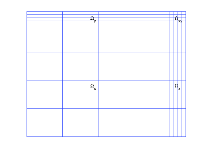
Figure 1: Dissection of $\Omega$ and triangulation $\Omega^{N}$.

The domain $\Omega$ is dissected into four parts as $\Omega=\Omega_{s}\cup\Omega_{x}\cup\Omega_{y}\cup\Omega_{xy}$(see FIG. 1), where

$$\Omega_{s}:=\left[0,1-\lambda_{x}\right]\times\left[0,1-\lambda_{y}\right], \Omega_{x}:=\left[1-\lambda_{x},1\right]\times\left[0,1-\lambda_{y}\right],$$

$$\Omega_{y}:=\left[0,1-\lambda_{x}\right]\times\left[1-\lambda_{y},1\right], \Omega_{xy}:=\left[1-\lambda_{x},1\right]\times\left[1-\lambda_{y},1\right].$$

We introduce the set of mesh points $\left\{(x_{i},y_{j})\in\Omega:i,\,j=0,\,\cdots,\,N\right\}$ defined by

$$x_{i}= 2i(1-\lambda_{x})/N, i=0,\,\cdots,\,N/2$$ for ,

$$x_{i}= 1-2(N-i)\lambda_{x}/N, i=N/2+1,\,\cdots,\,N$$ for

and

$$y_{j}= 2j(1-\lambda_{y})/N, j=0,\,\cdots,\,N/2$$ for ,

$$y_{j}= 1-2(N-j)\lambda_{y}/N, j=N/2+1,\,\cdots,\,N$$ for .

By drawing lines through these mesh points parallel to the $x$-axis and $y$-axis the domain $\Omega$ is partitioned into rectangles. This triangulation is denoted by $\Omega^{N}$(see FIG. 1). If $D$ is a mesh subdomain of $\Omega$, we write $D^{N}$ for the triangulation of $D$. The mesh sizes $h_{x,\tau}=x_{i}-x_{i-1}$ and $h_{y,\tau}=y_{j}-y_{j-1}$ satisfy

$$h_{x,\tau}= H_{x}:=\frac{1-\lambda_{x}}{N/2}, i=1,\,\cdots,\,N/2$$ for ,

$$h_{x,\tau}= h_{x}:=\frac{\lambda_{x}}{N/2}, i=N/2+1,\,\cdots,\,N$$ for

and

$$h_{y,\tau}= H_{y}:=\frac{1-\lambda_{y}}{N/2}, j=1,\,\cdots,\,N/2$$ for ,

$$h_{y,\tau}= h_{y}:=\frac{\lambda_{y}}{N/2}, j=N/2+1,\,\cdots,\,N$$ for .

The mesh sizes $h_{x,\tau}$ and $h_{y,\tau}$ satisfy

$$N^{-1}\leq H_{x},H_{y}\leq 2N^{-1}\quad\mbox{and}\quad C_{1}\varepsilon N^{-1}\ln N\leq h_{x},h_{y}\leq C_{2}\varepsilon N^{-1}\ln N,$$

where $C_{1}$ and $C_{2}$ are positive constants and independent of $\varepsilon$ and of the mesh parameter $N$. The above properties are essential when inverse inequalities are applied in our later analysis.

For the mesh elements we shall use two notations: $\tau_{ij}=[x_{i-1},x_{i}]\times[y_{j-1},y_{j}]$ for a specific element, and $\tau$ for a generic mesh rectangle.

2.2 The streamline diffusion finite element method

Let $V:=H^{1}_{0}(\Omega)$. On the above Shishkin mesh we define a finite element space

$$V^{N}:=\{v^{N}\in C(\bar{\Omega}):v^{N}|_{\partial\Omega}=0\text{ and $v^{N}|_{\tau}$ is bilinear, }\forall\tau\in\Omega^{N}\}.$$

In this case, the SDFEM reads as

(2.1) $$\left\{\begin{array}[]{lr}\text{Find $U\in V^{N}$ such that for all $v^{N}\in V^{N}$}\\ \varepsilon(\nabla U,\nabla v^{N})+(\boldsymbol{b}\cdot\nabla U+U,v^{N}+\delta\boldsymbol{b}\cdot\nabla v^{N})=(f,v^{N}+\delta\boldsymbol{b}\cdot\nabla v^{N}).\end{array}\right.$$

where $\delta=\delta(\boldsymbol{x})$ is a user-chosen parameter (see [3]).

We set

$$b:=\sqrt{b^{2}_{1}+b^{2}_{2}},\quad\boldsymbol{\beta}:=\genfrac{(}{)}{0.0pt}{0}{b_{1}}{b_{2}}/b,\quad\boldsymbol{\eta}:=\genfrac{(}{)}{0.0pt}{0}{-b_{2}}{b_{1}}/b\quad\mbox{and}\quad v_{\zeta}:=\boldsymbol{\zeta}^{T}\nabla v$$

for any vector $\boldsymbol{\zeta}$ of unit length. By an easy calculation one shows that

$$(\nabla w,\nabla v)=(w_{\beta},v_{\beta})+(w_{\eta},v_{\eta}).$$

We rewrite (2.1) as

$$\varepsilon(U_{\beta},v^{N}_{\beta})+\varepsilon(U_{\eta},v^{N}_{\eta})+(bU_{\beta}+U,v^{N}+\delta bv^{N}_{\beta})=(f,v^{N}+\delta bv^{N}_{\beta})$$

and, following usual practice, we set

$$\delta(\boldsymbol{x}):= N^{-1}, \boldsymbol{x}\in\Omega_{s}$$ if ,

$$\delta(\boldsymbol{x}):= 0,$$ otherwise.

For technical reasons in the later analysis, we increase the crosswind diffusion(see [4]) by replacing $\varepsilon(U_{\eta},v^{N}_{\eta})$ by $\hat{\varepsilon}(U_{\eta},v^{N}_{\eta})$ where

$$\tilde{\varepsilon}:=\max(\varepsilon,N^{-3/2})$$

and

$$\hat{\varepsilon}(\boldsymbol{x}):= \tilde{\varepsilon}, \boldsymbol{x}\in\Omega_{s}$$ ,

$$\hat{\varepsilon}(\boldsymbol{x}):= \varepsilon, \boldsymbol{x}\in\Omega\setminus\Omega_{s}$$ .

We now state our streamline diffusion method with artificial crosswind:

(2.2) $$\left\{\begin{array}[]{lr}\text{Find $U\in V^{N}$ such that for all $v^{N}\in V^{N}$}\\ B(U,v^{N})=(f,v^{N}+\delta bv^{N}_{\beta}),\end{array}\right.$$

with

(2.3) $$B(U,v^{N}):=(\varepsilon+b^{2}\delta)(U_{\beta},v^{N}_{\beta})+\hat{\varepsilon}(U_{\eta},v^{N}_{\eta})-b(1-\delta)(U,v^{N}_{\beta})+(U,v^{N}).$$

3 The discrete Green function

Let $\boldsymbol{x}^{\ast}$ be a mesh node in $\Omega$. The discrete Green’s function $G\in V^{N}$ associated with $\boldsymbol{x}^{\ast}$ is defined by

$$B(v^{N},G)=v^{N}(\boldsymbol{x}^{\ast}),\,\forall v^{N}\in V^{N}.$$

The weighted function $\omega$:

$$\omega(\boldsymbol{x}):=g\left(\frac{(\boldsymbol{x}-\boldsymbol{x}^{\ast})\cdot\boldsymbol{\beta}}{\sigma_{\beta}}\right)g\left(\frac{(\boldsymbol{x}-\boldsymbol{x}^{\ast})\cdot\boldsymbol{\eta}}{\sigma_{\eta}}\right)g\left(-\frac{(\boldsymbol{x}-\boldsymbol{x}^{\ast})\cdot\boldsymbol{\eta}}{\sigma_{\eta}}\right)$$

where

$$g(r)=\frac{2}{1+e^{r}}\quad\text{ for $r\in(-\infty,\infty)$}.$$

and $\sigma_{\beta}=kN^{-1}\ln N$ and $\sigma_{\eta}=k\tilde{\varepsilon}^{1/2}\ln N$.

$$|||G|||^{2}_{\omega}:=(\varepsilon+b^{2}\delta)\|\omega^{-1/2}G_{\beta}\|^{2}+\hat{\varepsilon}\|\omega^{-1/2}G_{\eta}\|^{2}+\frac{b}{2}\|(\omega^{-1})^{1/2}_{\beta}G\|^{2}+\|\omega^{-1/2}G\|^{2}$$

and

(3.1) $$|||G|||^{2}_{\omega}= B(\omega^{-1}G,G)-(\varepsilon+b^{2}\delta)((\omega^{-1})_{\beta}G,G_{\beta})$$

$$-\hat{\varepsilon}((\omega^{-1})_{\eta}G,G_{\eta})-b\delta(\omega^{-1}G,G_{\beta}).$$

Thus, we obtain

$$B(\omega^{-1}G,G) =B(E,G)+B((\omega^{-1}G)^{I},G)$$

$$=B(E,G)+(\omega^{-1}G)(\boldsymbol{x}^{\ast})$$

where $E:=\omega^{-1}G-(\omega^{-1}G)^{I}$.

Lemma 1.

If $\sigma_{\beta}=kN^{-1}\ln N$ and $\sigma_{\eta}=k\ln N\tilde{\varepsilon}^{1/2}$, then for $k>1$ sufficiently large and independent of $N$ and $\varepsilon$, we have

$$B(\omega^{-1}G,G)\geq\frac{1}{4}\||G|\|^{2}_{\omega}.$$

Proof.

From (3.1),we estimate the following terms.

$$(\varepsilon+\delta)\left|((\omega^{-1})_{\beta}G,G_{\beta})\right| \leq C(\varepsilon+\delta)^{1/2}\sigma^{-1/2}_{\beta}\cdot\|(\omega^{-1})^{1/2}_{\beta}G\|\cdot(\varepsilon+\delta)^{1/2}\|\omega^{-1/2}G_{\beta}\|$$

$$\leq C(\varepsilon+\delta)^{1/2}\sigma^{-1/2}_{\beta}\||G|\|^{2}_{\omega}$$

and

$$\hat{\varepsilon}\left|((\omega^{-1})_{\eta}G,G_{\eta})\right| \leq C\hat{\varepsilon}^{1/2}\sigma^{-1}_{\eta}\cdot\|\omega^{-1/2}G\|\cdot\hat{\varepsilon}^{1/2}\|\omega^{-1/2}G_{\eta}\|$$

$$\leq C\hat{\varepsilon}^{1/2}\sigma^{-1}_{\eta}\||G|\|^{2}_{\omega}$$

For $b\delta(\omega^{-1}G,G_{\beta})$, we make use of integration by parts.

From the definition of $\sigma_{\beta}$ and $\sigma_{\eta}$ and $\varepsilon\leq N^{-1}$, we take $k$ sufficiently large and we are done. ∎

Lemma 2.

If $\sigma_{\beta}=kN^{-1}\ln N$, with $k>0$ sufficiently large and independent of $N$ and $\varepsilon$. Then for each mesh point $\boldsymbol{x}^{\ast}\in\Omega\setminus\Omega_{xy}$, we have

$$\left|(\omega^{-1}G)(\boldsymbol{x}^{\ast})\right|\leq\frac{1}{16}\||G|\|^{2}_{\omega}+CN\ln N.$$

where $C$ is independent of $N$, $\varepsilon$ and $\boldsymbol{x}^{\ast}$.

Proof.

First let $\boldsymbol{x}^{\ast}\in\Omega_{s}$. Let $\tau^{\ast}$ be the unique triangle that has $\boldsymbol{x}^{\ast}$ as its north-east corner. Then

$$\left|(\omega^{-1}G)(\boldsymbol{x}^{\ast})\right| \leq CN\|G\|_{\tau^{\ast}}$$

$$\leq CN\underset{\tau^{\ast}}{\max}\left|(\omega^{-1})^{-1/2}_{\beta}\right|\cdot\|(\omega^{-1})^{-1/2}_{\beta}G\|_{\tau^{\ast}}$$

Calculating $(\omega^{-1})^{-1}_{\beta}(\boldsymbol{x})$ explicitly, we see that

$$(\omega^{-1})^{-1}_{\beta}(\boldsymbol{x})\leq C\sigma_{\beta}=CkN^{-1}\ln N\quad\forall\boldsymbol{x}\in\tau^{\ast}$$

Thus

$$\left|(\omega^{-1}G)(\boldsymbol{x}^{\ast})\right|\leq CN\ln N+\frac{1}{16}\||G|\|^{2}_{\omega}$$

by means of the arithmetic-geometric mean inequality.

Next, let $\boldsymbol{x}^{\ast}\in\Omega_{x}$.(The case $\boldsymbol{x}^{\ast}\in\Omega_{y}$ is similar.)Write $\boldsymbol{x}^{\ast}=(x_{i},y_{j})$. Then

$$\left|\omega^{-1}G(\boldsymbol{x}^{\ast})\right| =\left|G(\boldsymbol{x}^{\ast})\right|$$

$$=\left|\int^{1}_{x_{i}}G_{x}(t,y_{j})\mathrm{d}t\right|$$

$$\leq CH^{-1}_{y}\int^{1}_{x_{i}}\int^{y_{j+1}}_{y_{j}}\left|G_{x}(t,y)\right|\mathrm{d}y\mathrm{d}t$$

$$\leq CN(\varepsilon\ln N\cdot N^{-1})^{1/2}\|G_{x}\|_{\Omega_{x}}$$

$$\leq CN^{1/2}\ln^{1/2}N\||G|\|$$

where $G_{x}(t,y_{j})=\frac{G_{k,j}-G_{k-1,j}}{h_{x}}$ for $(t,y_{j})\in\tau_{kj}$.
Analysis: for the relation of boundary integral and domain integral, we analyze

$$\int^{1}_{x_{i}}\int^{y_{j+1}}_{y_{j}}\left|G_{x}(t,y)\right|\mathrm{d}y\mathrm{d}t=\sum^{N}_{k=i+1}h_{x}\int^{y_{j+1}}_{y_{j}}\left|f(y_{j})\frac{y_{j+1}-y}{H_{y}}+f(y_{j+1})\frac{y-y_{j}}{H_{y}}\right|\mathrm{d}y$$

where $f(y_{j})=\frac{G_{k,j}-G_{k-1,j}}{h_{x}}$ and $f(y_{j+1})=\frac{G_{k,j+1}-G_{k-1,j+1}}{h_{x}}$.
For $\Delta_{1}:=\int^{y_{j+1}}_{y_{j}}\left|f(y_{j})\frac{y_{j+1}-y}{H_{y}}+f(y_{j+1})\frac{y-y_{j}}{H_{y}}\right|\mathrm{d}y$, we have

$$\Delta_{1}= \frac{|f(y_{j})|+|f(y_{j+1})|}{2}H_{y}\geq\frac{1}{2}\max\{|f(y_{j}),|f(y_{j+1})|\}H_{y} f(y_{j})f(y_{j+1})\geq 0$$ if

$$\Delta_{1}= \frac{1}{2}\frac{f^{2}(y_{j})+f^{2}(y_{j+1})}{|f(y_{j+1})-f(y_{j})|}H_{y}\geq\frac{1}{4}\max\{|f(y_{j}),|f(y_{j+1})|\}H_{y} f(y_{j})f(y_{j+1})<0$$ if

∎

For $\forall v\in C^{2}(\tau)$, we have

$$|v_{x}|\leq C(|v_{\beta}|+|v_{\eta}|)$$

$$|v_{xx}|\leq C(|v_{\beta\beta}|+|v_{\beta\eta}|+|v_{\eta\eta}|)$$

Similarly, we have

$$|v_{\beta}|\leq C(|v_{x}|+|v_{y}|)$$

$$|v_{\beta\beta}|\leq C(|v_{xx}|+|v_{xy}|+|v_{yy}|)$$

Lemma 3.

Let $\tau\in\Omega^{N}$. Then

$$\|\omega^{1/2}D^{\alpha}E\|_{\Omega_{s}} \leq Ck^{-1/2}N^{1/2}|||G|||_{\omega}$$

$$\|\omega^{1/2}D^{\alpha}E\|_{\Omega^{N}\setminus\Omega_{s}} \leq Ck^{-1}\varepsilon^{-1/2}\ln^{-1}N|||G|||_{\omega}$$

where $H_{\tau}=\max\{h_{x,\tau},h_{y,\tau}\}$ and $|\alpha|=1$, $D^{\alpha}G$ are $G_{\beta}$ and $G_{\eta}$.

Proof.

Assume $p\in[1,\infty]$ and $g\in C^{3}(\tau)$. Then (see [2, Theorem 4])

$$\|(g-g^{I})_{x}\|_{L^{p}(\tau)} \leq C\left(h^{2}_{x,\tau}\|g_{xxx}\|_{L^{p}(\tau)}+h_{x,\tau}h_{y,\tau}\|g_{xxy}\|_{L^{p}(\tau)}+h^{2}_{y,\tau}\|g_{xyy}\|_{L^{p}(\tau)}\right)$$

$$+Ch_{x,\tau}\|g_{xx}\|_{L^{p}(\tau)},$$

$$\|(g-g^{I})_{y}\|_{L^{p}(\tau)} \leq C\left(h^{2}_{x,\tau}\|g_{xxy}\|_{L^{p}(\tau)}+h_{x,\tau}h_{y,\tau}\|g_{xyy}\|_{L^{p}(\tau)}+h^{2}_{y,\tau}\|g_{yyy}\|_{L^{p}(\tau)}\right)$$

$$+Ch_{y,\tau}\|g_{yy}\|_{L^{p}(\tau)}.$$

or (see [1, Comment 2.15])

$$\|(g-g^{I})_{x}\|_{L^{2}(\tau)} \leq Ch^{2}_{y,\tau}\|g_{xyy}\|_{L^{2}(\tau)}+Ch_{x,\tau}\|g_{xx}\|_{L^{2}(\tau)},$$

$$\|(g-g^{I})_{y}\|_{L^{2}(\tau)} \leq Ch^{2}_{x,\tau}\|g_{xxy}\|_{L^{2}(\tau)}+Ch_{y,\tau}\|g_{yy}\|_{L^{2}(\tau)}.$$

In the following analysis, $D^{\alpha}v$ denotes the directional derivative of $v$ along $\beta$ or $\eta$ for different orders. The following analysis makes use of the former estimates (The latter will make the analysis more shorter).

For $\tau\in\Omega^{N}$, we have

$$\|\omega^{1/2}E_{\beta}\|_{\tau}\leq C\underset{\tau}{\max}\omega^{1/2}(\|E_{x}\|_{\tau}+\|E_{y}\|_{\tau})$$

$$\leq C\underset{\tau}{\max}\omega^{1/2}\{h^{2}_{x,\tau}\|(\omega^{-1}G)_{xxx}\|_{\tau}+h_{x,\tau}\|(\omega^{-1}G)_{xx}\|_{\tau}+h_{x,\tau}H_{\tau}\|(\omega^{-1}G)_{xxy}\|_{\tau}$$

$$+H_{\tau}h_{y,\tau}\|(\omega^{-1}G)_{xyy}\|_{\tau}+h^{2}_{y,\tau}\|(\omega^{-1}G)_{yyy}\|_{\tau}+h_{y,\tau}\|(\omega^{-1}G)_{yy}\|_{\tau}\}$$

$$\leq Ch^{2}_{x,\tau}(\|(\omega^{-1})_{xxx}G\|_{\tau}+\|(\omega^{-1})_{xx}G_{x}\|_{\tau})+Ch_{x,\tau}(\|(\omega^{-1})_{xx}G\|_{\tau}+\|(\omega^{-1})_{x}G_{x}\|_{\tau})$$

$$+Ch^{2}_{y,\tau}(\|(\omega^{-1})_{yyy}G\|_{\tau}+\|(\omega^{-1})_{yy}G_{y}\|_{\tau})+Ch_{y,\tau}(\|(\omega^{-1})_{yy}G\|_{\tau}+\|(\omega^{-1})_{y}G_{y}\|_{\tau})$$

$$+Ch_{x,\tau}H_{\tau}(\|(\omega^{-1})_{xxy}G\|_{\tau}+\|(\omega^{-1})_{xx}G_{y}\|_{\tau}+\|(\omega^{-1})_{xy}G_{x}\|_{\tau}+\|(\omega^{-1})_{x}G_{xy}\|_{\tau})$$

$$+H_{\tau}h_{y,\tau}(\|(\omega^{-1})_{xyy}G\|_{\tau}+\|(\omega^{-1})_{xy}G_{y}\|_{\tau}+\|(\omega^{-1})_{yy}G_{x}\|_{\tau}+\|(\omega^{-1})_{y}G_{xy}\|_{\tau})$$

$$\leq CH_{\tau}^{2}\sum^{3}_{k=2}\sum_{\begin{array}[]{l}\scriptscriptstyle|\alpha|+|\gamma|=3\\ \scriptscriptstyle|\alpha|\geq k\end{array}}\|D^{\alpha}(\omega^{-1})D^{\gamma}G\|_{\tau}+CH_{\tau}\sum^{2}_{k=1}\sum_{\begin{array}[]{l}\scriptscriptstyle|\alpha|+|\gamma|=2\\ \scriptscriptstyle|\alpha|\geq k\end{array}}\|D^{\alpha}(\omega^{-1})D^{\gamma}G\|_{\tau}$$

where we have used the following analysis for $\sum_{|\alpha|=1,|\gamma|=2}D^{\alpha}(\omega^{-1})D^{\gamma}G$ :

$$\|(\omega^{-1})_{x}G_{xy}\|_{\tau} \leq C\|\sum_{|\alpha|=1}|D^{\alpha}(\omega^{-1})|\cdot G_{xy}\|_{\tau}$$

$$\leq C\underset{\tau}{\max}\sum_{|\alpha|=1}|D^{\alpha}(\omega^{-1})|\cdot\|G_{xy}\|_{\tau}$$

$$\leq Ch^{-1}_{y,\tau}\underset{\tau}{\max}\sum_{|\alpha|=1}|D^{\alpha}(\omega^{-1})|\cdot\|G_{x}\|_{\tau}$$

$$\leq Ch^{-1}_{y,\tau}\big{\|}\sum_{|\alpha|=1}|D^{\alpha}(\omega^{-1})|\cdot G_{x}\big{\|}_{\tau}.$$

The same analysis can be applied to $\|\omega^{1/2}E_{\eta}\|_{\tau}$.

For $\tau\in\Omega_{s}$, we have

$$\|\omega^{1/2}E_{\beta}\|_{\tau}\leq Ck^{-5/2}N^{-2}\big{[}(\sigma^{-5/2}_{\beta}+\sigma^{-3/2}_{\beta}\sigma^{-1}_{\eta}+\sigma^{-1/2}_{\beta}\sigma^{-2}_{\eta})\underset{\tau}{\max}(\omega^{-1})^{1/2}_{\beta}+\sigma^{-3}_{\eta}\underset{\tau}{\max}\omega^{-1/2}\big{]}\|G\|_{\tau}$$

$$+Ck^{-3/2}H^{2}_{\tau}\big{[}(\sigma^{-3/2}_{\beta}+\sigma^{-1/2}_{\beta}\sigma^{-1}_{\eta})\underset{\tau}{\max}(\omega^{-1})^{1/2}_{\beta}+\sigma^{-2}_{\eta}\underset{\tau}{\max}\omega^{-1/2}\big{]}\cdot N\|G\|_{\tau}$$

$$+Ck^{-3/2}H_{\tau}\big{[}(\sigma^{-3/2}_{\beta}+\sigma^{-1/2}_{\beta}\sigma^{-1}_{\eta})\underset{\tau}{\max}(\omega^{-1})^{1/2}_{\beta}+\sigma^{-2}_{\eta}\underset{\tau}{\max}\omega^{-1/2}\big{]}\|G\|_{\tau}$$

$$+C\underset{\tau}{\max}\omega^{1/2}H_{\tau}\sum_{|\alpha|=1}\|D^{\alpha}(\omega^{-1})\|_{L^{\infty}(\tau)}\cdot\sum_{|\gamma|=1}\|D^{\gamma}G\|_{\tau}$$

$$\leq Ck^{-1/2}N^{1/2}|||G|||_{\omega}$$

where we have used the estimates of $\omega^{-1}$, standard inverse estimates and Hölder inequalities. Similarly, we have

$$\|\omega^{1/2}E_{\eta}\|_{\Omega_{s}}\leq Ck^{-1/2}N^{1/2}|||G|||_{\omega}.$$

For $\tau\in\Omega^{N}\setminus\Omega^{N}_{s}$, we have

$$\|\omega^{1/2}E_{\beta}\|_{\tau}\leq Ck^{-5/2}H^{2}_{\tau}\big{[}(\sigma^{-5/2}_{\beta}+\sigma^{-3/2}_{\beta}\sigma^{-1}_{\eta}+\sigma^{-1/2}_{\beta}\sigma^{-2}_{\eta})\underset{\tau}{\max}(\omega^{-1})^{1/2}_{\beta}+\sigma^{-3}_{\eta}\underset{\tau}{\max}\omega^{-1/2}\big{]}\|G\|_{\tau}$$

$$+Ck^{-2}\varepsilon^{-1/2}H^{2}_{\tau}\big{[}\sigma^{-2}_{\beta}+\sigma^{-1}_{\beta}\sigma^{-1}_{\eta}+\sigma^{-2}_{\eta}\big{]}\underset{\tau}{\max}\omega^{-1/2}\cdot\varepsilon^{1/2}\sum_{|\gamma|=1}\|D^{\gamma}G\|_{\tau}$$

$$+Ck^{-3/2}H_{\tau}\big{[}(\sigma^{-3/2}_{\beta}+\sigma^{-1/2}_{\beta}\sigma^{-1}_{\eta})\underset{\tau}{\max}(\omega^{-1})^{1/2}_{\beta}+\sigma^{-2}_{\eta}\underset{\tau}{\max}\omega^{-1/2}\big{]}\|G\|_{\tau}$$

$$+Ck^{-1}\varepsilon^{-1/2}H_{\tau}\big{[}\sigma^{-1}_{\beta}+\sigma^{-1}_{\eta}\big{]}\underset{\tau}{\max}\omega^{-1/2}\cdot\varepsilon^{1/2}\sum_{|\gamma|=1}\|D^{\gamma}G\|_{\tau}$$

$$\leq Ck^{-1}\varepsilon^{-1/2}\ln^{-1}N|||G|||_{\omega}$$

Similarly, we have

$$\|\omega^{1/2}E_{\eta}\|_{\Omega\setminus\Omega_{s}}\leq Ck^{-1}\varepsilon^{-1/2}\ln^{-1}N|||G|||_{\omega}.$$

∎

Lemma 4.

Let $\tau\in\Omega^{N}_{s}$. Let $E=\omega^{-1}G-(\omega^{-1}G)^{I}$ where $(\omega^{-1}G)^{I}$ denote the bilinear function that interpolates to $\omega^{-1}G$ at the vertices of $\tau$. Then

$$\|\omega^{1/2}E\|_{\Omega_{s}}\leq Ck^{-1}N^{-1/2}|||G|||_{\omega}$$

$$\|\omega^{1/2}E\|_{\Omega\setminus\Omega_{s}}\leq Ck^{-1}\varepsilon^{1/2}|||G|||_{\omega}$$

where $H_{\tau}=\max\{h_{x,\tau},h_{y,\tau}\}$.

Proof.

We make use of the following standard interpolation error bounds

$$\|u-u^{I}\|_{L^{p}(\tau)}\leq h^{2}_{x,\tau}\|u_{xx}\|_{L^{p}(\tau)}+h^{2}_{y,\tau}\|u_{yy}\|_{L^{p}(\tau)}$$

where $p\in[1,\infty]$ and $u\in C(\overline{\tau})\cap W^{2,p}(\tau)$.

Then, we have

$$\|E\|_{\tau}\leq h^{2}_{x,\tau}\|(\omega^{-1}G)_{xx}\|_{\tau}+h^{2}_{y,\tau}\|(\omega^{-1}G)_{yy}\|_{\tau}$$

$$\leq CH^{2}_{\tau}\sum_{|\alpha|=2}\|D^{\alpha}(\omega^{-1})\cdot G\|_{\tau}+CH^{2}_{\tau}\|(|(\omega^{-1})_{\beta}|+|(\omega^{-1})_{\eta}|)\cdot(|G_{\beta}|+|G_{\eta}|)\|_{\tau}$$

$$\leq CH^{2}_{\tau}\left\{\|(\omega^{-1})_{\beta}G_{\beta}\|_{\tau}+\|(\omega^{-1})_{\beta}G_{\eta}\|_{\tau}+\|(\omega^{-1})_{\eta}G_{\beta}\|_{\tau}+\|(\omega^{-1})_{\eta}G_{\eta}\|_{\tau}\right\}$$

$$+CH^{2}_{\tau}\|\sum_{|\alpha|=2}|D^{\alpha}(\omega^{-1})|\cdot G\|_{\tau}.$$

From the above inequality, we have

$$\|\omega^{1/2}E\|_{\Omega_{s}}\leq Ck^{-1}N^{-1/2}|||G|||_{\omega}$$

and

$$\|\omega^{1/2}E\|_{\Omega\setminus\Omega_{s}}\leq Ck^{-1}\varepsilon^{-1/2}N^{-1}|||G|||_{\omega}.$$

Following the techniques of (see[5, Lemma 4.4]), we have

$$(\omega^{1/2}E)(\boldsymbol{x})=\int_{\boldsymbol{x}}^{\Gamma(\boldsymbol{x})}(\omega^{1/2}E)_{\eta}\mathrm{d}s$$

where $\boldsymbol{x}\in\Omega\setminus\Omega_{s}$, $\Gamma(\boldsymbol{x})\in\Gamma$ satisfies $(\boldsymbol{x}-\Gamma(\boldsymbol{x}))\cdot\beta=0$ and the following condition:

$$\begin{array}[]{r}\text{For $\forall\boldsymbol{y}\in\Gamma$, $(\boldsymbol{x}-\boldsymbol{y})\cdot\beta=0$,}\\ |\boldsymbol{x}-\Gamma(\boldsymbol{x})|=\underset{y}{\min}|\boldsymbol{x}-\boldsymbol{y}|.\end{array}$$

From the above representation of $\omega^{1/2}E$, we have

$$\|\omega^{1/2}E\|^{2}_{\Omega_{x}}=\int^{1-\lambda_{y}}_{\lambda_{0}}\int_{l(\boldsymbol{x}_{lu},\Gamma(\boldsymbol{x}_{lu}))}\left[\int_{\boldsymbol{x}}^{\Gamma(\boldsymbol{x})}(\omega^{1/2}E)_{\eta}\mathrm{d}s\right]^{2}\mathrm{d}\Omega$$

$$+\int_{1-\lambda_{x}}^{1}\int_{l(\boldsymbol{x}_{u},\Gamma(\boldsymbol{x}_{u}))}\left[\int_{\boldsymbol{x}}^{\Gamma(\boldsymbol{x})}(\omega^{1/2}E)_{\eta}\mathrm{d}s\right]^{2}\mathrm{d}\Omega+\int_{0}^{\lambda_{0}}\int_{l(\boldsymbol{x}_{ld},\Gamma(\boldsymbol{x}_{ld}))}\left[\int_{\boldsymbol{x}}^{\Gamma(\boldsymbol{x})}(\omega^{1/2}E)_{\eta}\mathrm{d}s\right]^{2}\mathrm{d}\Omega$$

$$\leq C\lambda^{2}_{x}\left\{\|(\omega^{1/2})_{\eta}E\|^{2}_{\Omega_{x}}+\|\omega^{1/2}E_{\eta}\|^{2}_{\Omega_{x}}\right\}$$

$$\leq C\varepsilon^{2}\ln^{2}N\left\{\sigma^{-2}_{\eta}\|\omega^{1/2}E\|^{2}_{\Omega_{x}}+\|\omega^{1/2}E_{\eta}\|^{2}_{\Omega_{x}}\right\}$$

$$\leq Ck^{-2}\varepsilon^{2}\ln^{2}N\{N^{3/2}\ln^{-2}N\cdot\varepsilon^{-1}N^{-2}+\varepsilon^{-1}\ln^{-2}N\}|||G|||^{2}_{\omega}$$

$$\leq Ck^{-2}\varepsilon|||G|||^{2}_{\omega}$$

where $\lambda_{0}=\frac{b_{1}}{b_{2}}\lambda_{x}$ and

• $x_{lu}\in\{(1-\lambda_{x},y):\lambda_{0}\leq y\leq 1-\lambda_{y}\}$;

• $x_{ld}\in\{(1-\lambda_{x},y):0\leq y\leq\lambda_{0}\}$;

• $x_{u}\in\{(x,1-\lambda_{y}):1-\lambda_{x}\leq x\leq 1\}$.

∎

Lemma 5.

If $\sigma_{\beta}=kN^{-1}\ln N$ and $\sigma_{\eta}=k\tilde{\varepsilon}^{1/2}\ln N$ , where $k>1$ sufficiently large and independent of $N$ and $\varepsilon$. Then

$$B((\omega^{-1}G)^{I}-\omega^{-1}G,G)\leq\frac{1}{16}\||G|\|^{2}_{\omega}.$$

Proof.

Cauchy-Schwarz s inequality gives

$$\left|B(E,G)\right| \leq(\varepsilon+b^{2}\delta)^{1/2}\|\omega^{1/2}E_{\beta}\|\cdot(\varepsilon+b^{2}\delta)^{1/2}\|\omega^{-1/2}G_{\beta}\|+\hat{\varepsilon}^{1/2}\|\omega^{1/2}E_{\eta}\|\cdot\hat{\varepsilon}^{1/2}\|\omega^{-1/2}G_{\eta}\|$$

$$+C\|\omega^{1/2}E\|\cdot\|\omega^{-1/2}G_{\beta}\|+\|\omega^{1/2}E\|\cdot\|\omega^{-1/2}G\|$$

From Lemma 3 and Lemma 4, we are done. ∎

Theorem 3.1.

Assume that $\sigma_{\beta}=kN^{-1}\ln N$ and $\sigma_{\eta}=k\tilde{\varepsilon}^{1/2}\ln N$, where $k>0$ is sufficiently large and independent of $\varepsilon$ and $N$. Let $\boldsymbol{x}^{*}\in\Omega\setminus\Omega_{xy}$. Then for each nonnegative integer $\upsilon$, there exists a positive constant $C=C(\upsilon)$ and $K=K(\upsilon)$ such that

$$\|G\|_{W^{1,\infty}(\Omega_{s}\setminus\Omega^{\prime}_{0})}\leq CN^{-\upsilon},$$

$$\varepsilon|G|_{W^{1,\infty}((\Omega_{x}\cup\Omega_{y})\setminus\Omega^{\prime}_{0})}+\|G\|_{L^{\infty}((\Omega_{x}\cup\Omega_{y})\setminus\Omega^{\prime}_{0})}\leq CN^{-\upsilon}$$

and

$$\varepsilon|G|_{W^{1,\infty}(\Omega_{xy}\setminus\Omega^{\prime}_{0})}+\|G\|_{L^{\infty}(\Omega_{xy}\setminus\Omega^{\prime}_{0})}\leq C\varepsilon^{-1/2}N^{-\upsilon}.$$

Proof.

On $\Omega_{s}$, we apply an inverse estimate.
On $\Omega\setminus\Omega_{s}$ the application of an inverse estimate does not yield a satisfactory result, so we use a different technique.

Let $\boldsymbol{x}\in\Omega_{x}\setminus\Omega^{\prime}_{0}$ be arbitrary. Starting from $\boldsymbol{x}$ we choose a polygonal curve $\Gamma\subset(\Omega\setminus\Omega_{xy})\setminus\Omega^{\prime}_{0}$ that joints $\boldsymbol{x}$ with some point on outflow boundaries. If $(\boldsymbol{x}-\boldsymbol{x}^{\ast})\cdot\eta<0$, we can choose $\Gamma$ as a line parallel to $\beta$. If $(\boldsymbol{x}-\boldsymbol{x}^{\ast})\cdot\eta>0$, the situation is a little complicated. We can choose $\Gamma$ as follows:
In $\Omega_{x}\setminus\Omega^{\prime}_{0}$, we choose the direction of $\Gamma$ along $\eta$ or the negative direction of $x$-axis so that $\Gamma\cap\Omega_{xy}=\Phi$. In $(\Omega_{s}\cup\Omega_{y})\setminus\Omega^{\prime}_{0}$, we choose the direction of $\Gamma$ along $\eta$ or the positive direction of $y-$axis.
Let $T^{N}$ be the set of mesh rectangle $\tau$ in $(\Omega\setminus\Omega_{xy})\setminus\Omega^{\prime}_{0}$ that $\Gamma$ intersects. Note that the length of the segment of $\Gamma$ that lies in each $\tau$ is at most $C\varepsilon N^{-1}\ln N$ if $\tau\in\Omega_{x}$ or $\tau\in\Omega_{y}$.

Then, by the fundamental theorem of calculus and inverse estimates in different domain, we can obtain the results. ∎

References

- [1] T. Apel. Anisotropic Finite Elements: Local Estimates and Applications. B. G. Teubner Verlag, Stuttgart, 1999.
- [2] T. Apel and M. Dobrowolski. Anisotropic interpolation with applications to the finite element method. Computing, 47:277–293, 1992.
- [3] C. Johnson. Numerical Solution of Partial Differential Equations by the Finite Element Method. Cambridge University Press, Cambridge, 1987.
- [4] C. Johnson, A. H. Schatz, and L. B. Wahlbin. Crosswind smear and pointwise errors in streamline diffusion finite element methods. Mathematics of Computation, 49(179):25–38, 1987.
- [5] T. Linß and M. Stynes. The SDFEM on shishkin meshes for linear convection–diffusion problems. Numer. Math., 87:457–484, 2001.