How well do starlab and nbody compare? II: Hardware and accuracy

Abstract

Most recent progress in understanding the dynamical evolution of star clusters relies on direct $N$-body simulations. Owing to the computational demands, and the desire to model more complex and more massive star clusters, hardware calculational accelerators, such as GRAPE special-purpose hardware or, more recently, GPUs (i.e. graphics cards), are generally utilised. In addition, simulations can be accelerated by adjusting parameters determining the calculation accuracy (i.e. changing the internal simulation time step used for each star).

We extend our previous thorough comparison (Anders et al. 2009) of basic quantities as derived from simulations performed either with starlab/kira or nbody6. Here we focus on differences arising from using different hardware accelerations (including the increasingly popular graphic card accelerations/GPUs) and different calculation accuracy settings.

We use the large number of star cluster models (for a fixed stellar mass function, without stellar/binary evolution, primordial binaries, external tidal fields etc) already used in the previous paper, evolve them with starlab/kira (and nbody6, where required), analyse them in a consistent way and compare the averaged results quantitatively. For this quantitative comparison, we apply the bootstrap algorithm for functional dependencies developed in our previous study.

In general we find very high comparability of the simulation results, independent of the used computer hardware (including the hardware accelerators) and the used $N$-body code. For the tested accuracy settings we find that for reduced accuracy (i.e. time step at least a factor 2.5 larger than the standard setting) most simulation results deviate significantly from the results using standard settings. The remaining deviations are comprehensible and explicable.

1 Introduction

In recent years, the modelling of star populations strongly advanced due to stellar dynamical studies. The fields covered comprehend a wide range of research questions, such as the modelling of individual star clusters (e.g. Baumgardt et al. 2003; Hurley et al. 2005; Heggie & Giersz 2009; Harfst et al. 2010; Zonoozi et al. 2011), star cluster systems (e.g. Vesperini et al. 2003), populations of “exotic” stellar objects (Portegies Zwart et al. 2004 - massive black holes, Umbreit et al. 2008 - blue stragglers, Decressin et al. 2010 - second populations of globular cluster stars, Gualandris et al. 2005; Gvaramadze et al. 2008; Fujii & Portegies Zwart 2011 - run-away stars) etc.

The major codes used in this field are the family of nbodyx codes (Aarseth 1999) and the starlab environment with its $N$-body integrator kira (Portegies Zwart et al. 2001). Both codes are continuously expanded and improved, including the ability for the use of hardware dedicated to improve the simulation capabilities (in terms of simulation duration and available population size). This includes advances in software development (such as parallelisation, see e.g. Harfst et al. 2007; Spurzem et al. 2008; Portegies Zwart et al. 2008) and the use of dedicated hardware, e.g. GRAPEs (Ebisuzaki et al. 1993; Makino et al. 2003), more recently the use of GPUs (Portegies Zwart et al. 2007; Gaburov et al. 2009; Nitadori & Aarseth 2011; Moore & Quillen 2011), supercomputers/computer clusters (Harfst et al. 2007) and large area networks, such as GRID (Groen et al. 2011).

Additional $N$-body codes are emerging, such as MYRIAD (Konstantinidis & Kokkotas 2010, GRAPE-enabled), NBSymple (Capuzzo-Dolcetta et al. 2011, GPU-enabled) and AMUSE (Portegies Zwart et al. 2009, a compilation of various modules for gravitational dynamics, stellar evolution, radiative transfer and hydrodynamics, which can become independently combined). GPUs are also applied in an additional wide range of astrophysical simulation environments (Ford 2009; Schive et al. 2010; Thompson et al. 2010). Their general availability and useability for computationally intensive astrophysical modelling will continue the rise of GPU usage.

Despite their extensive use and computational specialities (see Sects. 2 and 4.2), a detailed study concerning the reliability and comparability of simulations performed is missing. Important factors, which are studied in the present work, include the use of various computer hardware (including diverse special-purpose hardware to accelerate the simulations) and simulation accuracy settings. The named factors determine the used calculation accuracy and therefore the accuracy to trace accurately fast important phases of star cluster evolution. Potentially, this can lead to incommensurable simulation results, although starting configuration and physical treatment are equivalent.

In Sect. 2 describes the used hardware and software, including their limitations in calculation accuracy. Sect. 3 summarizes the used simulation and analysis methods. In Sect. 4 the simulation results are explained and analysed, with a summary of all results and drawn conclusions in Sect. 5.

2 Utilised hardware and software

We used 3 PCs for these simulations, whose specifications are summarised in Table 1. The use of these 3 PCs was necessary to allow testing the sensitivity of the results on the PC architecture and the availability of varying accelerator hardware. The labels “PC1”, “PC2” and “PC3” will be used to indicate the use of solely the CPU, without the available accelerator hardware. “PC1/GPU”, “PC2/GRAPE” and “PC3/GPU” indicate the usage of the available accelerator hardware.

Table 1: Specifications of PCs used

specification	PC1	PC2	PC3
Processor	Quad Core Intel Q9300	Dual Core Intel Xeon	Dual Core AMD Opteron
Operating system	Debian 4.0	Red Hat 2.6.9-67	Debian 2.6.24.7
C compiler	gcc 4.2	gcc 3.4.6	gcc 4.3.2
Special hardware	GeForce 9800 GX2	GRAPE6-BLX64	GeForce 9800 GX2
Special hardware libraries	Sapporo v1.5	g6bx-0515	GPU module by K. Nitadori
$N$-body software	starlab 4.4.4	starlab 4.4.4	nbody6

For the majority of tests we use the starlab software package. Where we supplement these with simulations made with nbody we use nbody6, contrary to our previous study (Anders et al. 2009, hereafter “Paper I”) where we used nbody4. nbody6 presents a significant enhancement of required computational time due to the AC neighbour scheme (Ahmad & Cohen 1973 for the AC neighbour scheme and Aarseth 2001 for the nbody implementation).

2.1 Possible reasons for simulation differences

Numerical modeling of $N$-body systems, such as star clusters, usually involves long-term simulations. It is therefore necessary to understand the influence of different errors on the outcome. In a very basic case of a direct integration, there are two contributions to the overall error: one due to the time integration and one due to the accuracy of force calculations. In the idealistic case these two should be balanced, but in the majority of codes (e.g. nbody4, starlab, phiGrape Harfst et al. 2008, Myriad Konstantinidis & Kokkotas 2010) a simple direct summation method is employed to compute forces, whereas nbody6 uses the Ahmad-Cohen neighbour scheme. While this, in principle, should result in exact accelerations, in practice, due to limited precision, several factors affect the result. For example, the order in which partial forces are added affects the accuracy: if the partial forces are added from the weakest to strongest the total force on a particle is more accurate compared to the one if the summation is done in reverse or in arbitrary order. This is exacerbated if the precision of the force accumulation is below a certain threshold which depends on the system being modelled. On CPU, a generic double precision force loop usually adds up partial forces in IEEE double precision arithmetics, which, is safe to say, results in the most accurate force. On special purpose accelerations (such as GRAPE or GPU), for performance considerations, the summations is done in lower precision (e.g. Makino et al. 2003; Nitadori 2008; Gaburov et al. 2009). For example, Nitadori (2008) and Gaburov et al. (2009) use two single precision numbers to emulate double precision, and the second authors conduct force accumulation in single precision. The emulation of double precision is inherently less precise (2x23 bits mantissa) compared to IEEE double precision (53 bits mantissa), and its long-term errors are poorly understood. This may potentially inflict damage to long-term integrations.

In direct $N$-body simulations the error is usually due to time integration (among other errors coming from binary and multiple treatment, stellar evolution, close encounter treatment) rather than force summation. Generally in $N$-body codes, the time-step is defined by the Aarseth criterion (Aarseth 2003) which is usually scaled by an “accuracy parameter” $\eta$. The time-step size monotonically depends on $\eta$ and changes in this parameter have proportional changes in the value of the time-step. In a generally employed $4^{th}$ order Hermite scheme, the error decreases as the $4^{th}$ order of the time-step, and for a realistic time-step criterium which provides a good balance between duration of simulations and accuracy, this error remains dominant. Furthermore, time integration error has similar properties among different codes due to its simpler nature.

If $\eta$ is increased above a certain value, the time integration errors become intolerable, for example close encounters and dynamical binary integration become inaccurately simulated, but consistent among different codes. If $\eta$ is decreases beyond a certain value, the dominant source of error becomes force computation, which varies among different implementations to a large degree. While this produces more accurate results, the outcome from different codes may show large scatter in sensitive quantities, such as energy conservation error, due to possibly significantly different force summation (or other) errors, rather than similar time integration errors, influence long-term simulations. In this paper we explore a range of $\eta$ parameters to identify their influence on the simulation results.

3 Methods

In this section we will summarize the methods developed in Paper I and applied in the present paper. For additional details see Paper I.

3.1 Standard setup

We used start models from the predecessor study. They were created using starlab (and, where necessary, transformed into the nbody file format) and have the following characteristics

• 1024 (1k) particles

• Salpeter (1955) stellar mass function, with the highest mass = 10 $\times$ lowest mass

• no primordial binaries

• Plummer (1911) sphere initial density profile

There are 50 start models, with identical parameters but varying statistical realisations.

All simulations were performed with the following settings:

• no stellar/binary star evolution

• no external tidal field

• duration of simulation: 1000 $N$-body time units (i.e., until well after core collapse, which occurs around 60 $N$-body time units, see Paper I).

Unless otherwise specified, the simulations were performed using

• hardware acceleration: GeForce 9800GX2 GPU

• calculation accuracy parameter $\eta$=$\eta_{\rm STARLAB}$=0.1 for starlab, equivalent to $\eta_{\rm NBODY}$=0.01 (due to a different definition of the accuracy parameter in starlab and in nbody6, see Sect. 4.2). All quoted accuracy parameters are given as $\eta$=$\eta_{\rm STARLAB}$.

3.2 Analysis of $N$-body simulation snapshots

As we want to trace differential effects between our settings (i.e., nbody6 vs. starlab, solely CPU vs. CPU+GRAPE vs. CPU+GPU, different accuracy parameters) we need to ensure that output from different simulations is treated identically. The main difficulty arises when comparing nbody6 and starlab output, as the output content and format is very different. E.g., nbody6 output does not contain detailed information about binaries, while starlab output contains information on binary/triple/higher order hierarchies.

We therefore reduce the format of each simulation output to the most basic one possible, only containing for each star its mass and vectors for its position and velocity. Binaries and higher order hierarchies are split up into their components. Other possibly present information is removed.

We then split the series of output into individual snapshots, pass them through kira, the $N$-body integrator of the starlab package, which evolves them for the 1/32^th part of an $N$-body time unit. This procedure rebuilds the binary/higher order hierarchy structure, and stores it accessibly in the resulting snapshot. All snapshots with rebuilt hierarchy structure are then analysed using tools available within the starlab package. In Paper I we investigated the reliability of this procedure and did not find significant biases (except for the spurious re-building of multiple systems in the outer cluster regions, which are not subject of the present study). In addition, we calculate the change of total energy per N-body time unit as a measure of the energy conservation.

Results of this procedure are time series of cluster parameters (like core radius, virial ratio, etc) and binary parameters (here only investigated at the end of the simulation; as shown in Paper I testing at different times gives comparable results but poorer statistics). For the further analysis, results from the 50 individual runs per simulation setting are combined: the lists of binary parameters are merged, while for the overall cluster parameters a median time series and the 16/84 per cent quantiles are calculated.

3.3 Analyses of the simulation outcome

In this section we want to summarize the methods used for the analysis of the $N$-body data. Many of the analysis results are given as probabilities. We will adopt the following (commonly used) nomenclature when discussing the significance level of statistical test results

• highly significant: p-value $<$ 1%

• significant: p-value $<$ 5%

• weakly significant: p-value $<$ 10%.

“Multiple testing”: if we perform 100 independent tests, a fraction of the order of $10\%$ of p-values below $0.1$ will arise by chance even if none of the test null hypotheses is wrong. As we analyse various star cluster parameters of a large number of simulations, we need to take “multiple testing” into account.

3.3.1 Binary and escaper parameters

We will analyse the parameters of dynamically created binaries (semi-major axis, eccentricity, mass ratio, binding energy) and the energy distributions of stars escaping from the cluster.

Differences between two such distributions for two different simulation setups are evaluated using a Kuiper test (Kuiper 1962), an advanced KS test (for the KS test and Kuiper test see, e.g., Numerical Recipes Press et al. 1992). A Kuiper test returns the probability that two distributions are drawn from the same parent distribution (or, more accurately, the probability that one is wrongly rejecting the null hypothesis “The two distributions are drawn from the same parent distribution.”, which in most cases is equivalent).

3.3.2 Time series

In Paper I we developed a bootstrap algorithm for functional dependencies and applied it to time series similar to the ones studied in the present work. For example, we want to quantitatively compare the time evolution of the core radius (and of other parameters) for two different simulations setups.

First, we introduce a measure of the difference between two time series’ (or, more general, between two functional dependencies). Assume we have two functional dependencies of one parameter from the independent variable $x$: $y_{1}(x)$ and $y_{2}(x)$. For each $x$ these dependencies have uncertainties $\sigma_{1}(x)$ and $\sigma_{2}(x)$. The relative difference between the functional dependencies at a given $x$ is then:

$$\delta_{12}(x)=\frac{y_{1}(x)-y_{2}(x)}{\sqrt{\sigma_{1}(x)^{2}+\sigma_{2}(x)^{2}}}$$ (1)

We then define the “difference between functions 1 and 2” as

$$\Delta_{12}=\frac{1}{N}\cdot\left|\sum_{x}\delta_{12}(x)\right|$$ (2)

where $N$ is the number of datapoints used for the statistic. We consider only the absolute value, as we want to have a measure of the size of the difference, but not necessarily its direction. In addition, this ensures $\Delta_{12}\equiv\Delta_{21}$.

Equivalently we define the “absolute difference between functions 1 and 2” as

$$\Gamma_{12}=\frac{1}{N}\cdot\sum_{x}\left|\delta_{12}(x)\right|$$ (3)

While $\Delta_{12}$ is more sensitive to systematic offsets, $\Gamma_{12}$ traces also statistical fluctuations.

We then utilise this measure of difference between two time series’ to design a bootstrap-like algorithm to quantify the significance of this difference.

We calculate 300 test clusters with starlab using the standard settings (i.e., using PC1/GPU and with $\eta$=0.1), and the same analysis routines as for the other clusters.

From these test clusters we randomly select sets of 50 clusters each (i.e. the number of clusters in the main simulations) with replacement, and calculate for each parameter the median $y^{T}(x)$ and quantiles $\sigma^{T}(x)$.

We build 2000 such sets. Out of those we randomly select two sets (again with replacement) and derive the individual values of $\Delta_{12}^{T}$ and $\Gamma_{12}^{T}$. We repeat this procedure 10000 times to estimate the $\Delta_{12}^{T}$ and $\Gamma_{12}^{T}$ test distributions for each parameter. As all test clusters are calculated with the same settings, the $\Delta_{12}^{T}$ and $\Gamma_{12}^{T}$ test distributions represent the null hypothesis “functions 1 and 2 are drawn from the same parent distribution”. By comparing these test distributions with the values derived from the main simulations $\Delta_{12}^{S}$ and $\Gamma_{12}^{S}$ we can quantify the fraction of data in the test distribution with $\Delta_{12}^{T}$ or $\Gamma_{12}^{T}$ more deviating than the values derived from the main simulations $\Delta_{12}^{S}$ or $\Gamma_{12}^{S}$. This value serves as measure of how similar the two main simulations are.

In order to avoid applying the test statistic to highly correlated data, which appears for the earliest timesteps (as all runs share the same type of start models, only different stochastic realisations) and which is beyond the area of application of the test statistic, we start the summation in Eq. 2 and 3 at 20 $N$-body time units. This is sufficiently well before core collapse, which appears at about 60 $N$-body time units (see Paper I), to capture the systems’ behaviour during this important epoch. As we have shown in Paper I, the influence of varying this start time slightly is small and does not change the conclusions drawn.

4 Results

In this section we will compare simulations made for a number of specifications.

The quantitative test results are tabulated in Appendix B and summarized in Sect. 5. Visual presentations of time series for selected results are provided in Appendix A. .

4.1 Different hardware, using starlab

We have performed simulations on PC1 and PC2. For each PC we realised one set of simulations with the installed accelerator hardware and one set without hardware acceleration.

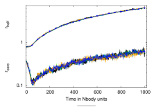
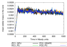
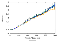
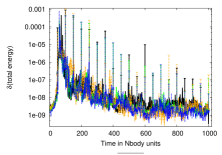
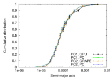
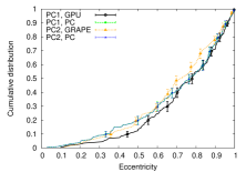
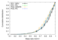
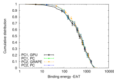
Figure 1: Comparison of simulations using starlab and various hardware. The lines show the median values, the error bars give the uncertainty ranges from the 50 individual runs. Shown are the time evolutions of the core radius (top left, bottom lines), half-mass radius (top left, upper lines), the objects’ mean mass in the core = measure for mass segregation (top right), virial ratio (bottom left) and change in total energy during 1 $N$-body time unit (bottom right).

Figure 2: Comparison of binary parameters from simulations using starlab and various hardware after 1000 $N$-body time units (i.e., well after core collapse). Shown are the cumulative distributions of the semi-major axis (top left), the eccentricity (top right), mass ratio of secondary to primary (bottom left) and the binding energy (bottom right). The lines show the data, the error bars give the uncertainty ranges from bootstrapping (at every 20^th data point only, for clarity).

The results are visualised in Figs. 2 and 2. The agreement appears to be very good, with possible exceptions being the evolution of the kinetic energy (though with large error bars, only the virial ratio is shown for consistency with the other sections) and the cumulative eccentricity and mass ratio distributions of the dynamically created binaries. The quantitative measures (our bootstrap algorithm for integrated cluster properties, and the Kuiper test for the properties of binaries and escaping stars), shown in Tables 2 - 5, generally confirm the good agreement. The following issues are found

• significant differences: kinetic energy of stars escaping from the cluster for
  #1.1 PC1 $\Leftrightarrow$ PC1/GPU
  and differences (visible in Fig. 2) in the mass ratio distributions for
  #1.1 PC1 $\Leftrightarrow$ PC1/GPU
  #1.2 PC1/GPU $\Leftrightarrow$ PC2/GRAPE

• weakly significant: the $\Delta_{12}$ test of King W₀ and the potential energy for
  #1.3 PC2 $\Leftrightarrow$ PC2/GRAPE

• statistically insignificant: differences in the total kinetic energy of all stars and the binary eccentricity distributions (visible in Fig. 2)

Deviations in the mass ratio distributions can originate from the stochastical process of two-body interaction processes. The number and level of the remaining deviations is in agreement with “multiple testing”, i.e. the occurence of statistical disagreement based on large numbers of tests. Therefore, $N$-body simulations based on equivalent start conditions and $N$-body code (here starlab) produce highly comparable results, independent of the computer hardware (including the accelerator hardware).

4.2 Accuracy settings

Using PC1/GPU, we test the impact of the calculation accuracy.

The “calculation accuracy” is determined by a dimensionless constant $\eta$ in the formula determining the integration time step (see Aarseth 2003, Sect. 2.3)

$$\Delta t_{i} = \sqrt{\eta_{nbody}\frac{(|\mathbf{F}||\mathbf{F^{(2)}}|+|\mathbf{F}|^{2})}{|\mathbf{F^{(1)}}||\mathbf{F^{(3)}}|+|\mathbf{F^{(2)}}|^{2}}}$$ (4)

$$= \eta_{starlab}\sqrt{\frac{(|\mathbf{F}||\mathbf{F^{(2)}}|+|\mathbf{F}|^{2})}{|\mathbf{F^{(1)}}||\mathbf{F^{(3)}}|+|\mathbf{F^{(2)}}|^{2}}}$$

where $\mathbf{F}$ is the force affecting particle $i$ and $\mathbf{F}^{(j)}$ its $j$-th time derivative.

Due to the slightly different definitions used by starlab and nbody is $\eta_{\rm starlab}$=$\sqrt{\eta_{\rm nbody}}$. In the remainder of the paper we will express all accuracy settings as $\eta$=$\eta_{\rm starlab}$.

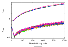
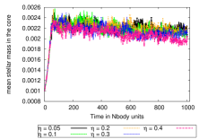
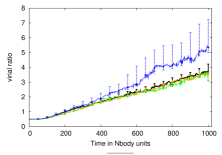
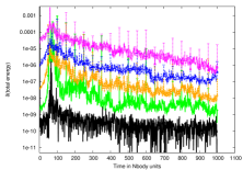
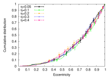
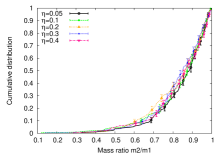
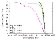
Figure 3: Comparison of simulations using starlab and various accuracy settings, all using PC1 and GPU. The lines show the median values, the error bars give the uncertainty ranges from the 50 individual runs. Shown are the time evolutions of the core radius (top left, bottom lines), half-mass radius (top left, upper lines), the objects’ mean mass in the core = measure for mass segregation (top right), virial ratio (bottom left; $\eta$=0.4 is not shown due to very large deviations and error bars) and change in total energy during 1 $N$-body time unit (bottom right).

Figure 4: Comparison of binary parameters from simulations using starlab and various accuracy settings after 1000 $N$-body time units (i.e., well after core collapse). All using PC1 and GPU. Shown are the cumulative distributions of the semi-major axis (top left), the eccentricity (top right), mass ratio of secondary to primary (bottom left) and the binding energy (bottom right). The lines show the data, the error bars give the uncertainty ranges from bootstrapping (at every 20^th data point only, for clarity).

The results are displayed in Figs. 4 and 4.

In most panels, the simulations with the largest accuracy parameter (i.e., the “worst” accuracy) studied are clearly offset from the other simulations. The other simulations seem to provide quite comparable results, except for the change in total energy during 1 $N$-body time unit (i.e., a measure for energy conservation). The change in total energy reduces with lowering the accuracy parameter $\eta$ both before and after core collapse, i.e. total energy becomes better preserved when improving accuracy.

These findings are confirmed by the quantitative measures from our tests:

• (highly) significant: most results for the $\eta$=0.3 and $\eta$=0.4 runs strongly deviate from the results using the standard settings, independent of used hardware and studied parameter. For the $\eta$=0.25 runs, the results depend on the studied parameter: one part of the results follow the standard setting results, while for the other parameters the results deviate from the standard setting runs similarly to the $\eta$=0.3 run results (no clear correlation between studied parameter and found deviation)

• (highly) significant: the change in total energy during 1 $N$-body time unit (i.e. our measure for energy conservation) is deviating from the standard settings for almost all runs

• (highly) significant: additional individual deviations are found, without a specific correlation with simulation settings, used hardware or studied parameter.

The strongly deviating results for $\eta$=0.3 and $\eta$=0.4 runs (and partially the $\eta$=0.25 runs) represent strong discouragement for such “inaccurate” simulations.

The results for the energy conservation is expected. The better the simulation accuracy the better even slight effects are traced. These slight effects, e.g. individual close encounters or binary evolution, have strong impact on the conservation of the system’s energy.

The number and level of additional deviations exceeds the expectations based on “multiple testing”, also without the $\eta$=0.3 and $\eta$=0.4 runs. The level of accuracy changes the simulation results slightly but cumulatively, therefore fundamental agreement for all studied parameters from simulations using different accuracy settings is not assured.

4.3 starlab vs. nbody6

We have performed simulations on PC1 and PC3. For each PC we realised one set of simulations with the installed GPUs and one set without hardware acceleration. The starlab simulations were performed with $\eta_{\rm starlab}$ = 0.1, while the nbody6 simulations were performed with $\eta_{\rm starlab}\approx$ 0.15 ($\eta_{i}=\sqrt{0.02}$ and $\eta_{r}=\sqrt{0.03}$). As shown in Sect. 4.2, these settings give comparable results.

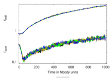
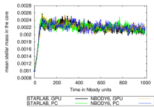
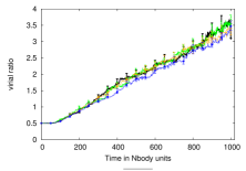
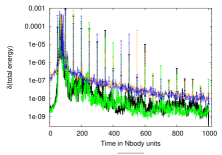
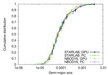
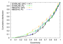
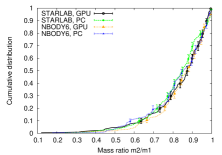
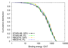
Figure 5: Comparison of simulations using starlab or nbody6, with either GPU acceleration or no hardware acceleration. The lines show the median values, the error bars give the uncertainty ranges from the 50 individual runs. Shown are the time evolutions of the core radius (top left, bottom lines), half-mass radius (top left, upper lines), the objects’ mean mass in the core = measure for mass segregation (top right), virial ratio (bottom left) and change in total energy during 1 $N$-body time unit (bottom right).

Figure 6: Comparison of binary parameters from simulations using starlab or nbody6, with either GPU acceleration or no hardware acceleration, after 1000 $N$-body time units (i.e., well after core collapse). Shown are the cumulative distributions of the semi-major axis (top left), the eccentricity (top right), mass ratio of secondary to primary (bottom left) and the binding energy (bottom right). The lines show the data, the error bars give the uncertainty ranges from bootstrapping (at every 20^th data point only, for clarity).

The results are shown in Figs. 6 and 6. They indicate potential deviations in kinetic energy for the nbody6 runs using PC3, in the change of total energy (during 1 $N$-body time unit) between nbody6 and starlab runs, and in binary eccentricity for the GPU runs using either nbody6 or starlab.

Our quantitative tests confirm the deviations for the change in total energy during 1 $N$-body time unit: It is bigger (i.e. energy conservation is worse) for nbody6 as compared to starlab. This agrees with our earlier finding for nbody4 vs. starlab in Paper I.

The remaining expectations, based on visual examination of Figs. 6 and 6, are not confirmed. Our statistical tests indicate deviations in

• significant: the time evolution of r_max (i.e., the distance of the furthest star from the cluster center) when comparing simulations made with starlab and nbody6, both without hardware acceleration

• weakly significant: the binary mass ratio distribution for #3.2 PC1 $\Leftrightarrow$ PC3

• weakly significant: the distribution the kinetic energy of stars escaping the cluster for #3.1 PC1/GPU $\Leftrightarrow$ PC3/GPU

These results are partially inconsistent with our previous study of starlab vs nbody4 in Paper I. In Paper I no significant deviations in r_max were found, the binary mass ratio distributions were different (the probability of both being drawn from the same parent distribution was determined to be 14.9%, slightly larger than required for a statistically slightly significant deviation) and for the kinetic energy of stars escaping the cluster no significant deviations was found. The detected differences in the present work are expected to originate from code differences between nbody4 and nbody6 (code enhancements, such as the AC neighbour scheme) or starlab (version 4.4.2) and starlab (version 4.4.4) (which included bug fixes).

The results for the time evolution of r_max and the binary mass ratio distributions are based on processes with strong statistical effects as these quantities are affected by rare events, e.g. direct two-body interaction processes. In general, the number and level of deviations agrees with the expectations from “multiple testing”. These results allow reliable comparisons of nbody6 and starlab simulations, based on comparable input parameters and independent of the used computer hardware.

5 Summary of results & conclusions

All of the quantitative test results are shown in Tables 2 - 5. They are based on 50 input models and their consistently analysed output.

From these tables the following picture emerges

• in general, the results obtained from $N$-body simulations in various configurations are well comparable (with some exceptions which will be discussed as follows), independent of the computer hardware, the accelerator type and $N$-body code used.

• results with too coarse accuracy (for our tests, $\eta_{STARLAB}$ = 0.3 and $\eta_{STARLAB}$ = 0.4, partially $\eta_{STARLAB}$ = 0.25) give strongly significantly deviating results in a variety of quantities, hence should be avoided.

• the quantity which shows the highest sensitivity to the configuration used is the energy conservation (here described by the change of total cluster energy during one $N$-body time unit). While it seems to be unaffected by the hardware used, it changes strongly with the accuracy parameter $\eta$, and between nbody6 and starlab. The behaviour with accuracy parameter is expected and desired. The differences between nbody6 and starlab are comparable to our earlier finding when comparing nbody4 and starlab in Paper I.

• the significant deviation found for some configurations in the temporal evolution of r_max (distance of furthest star from cluster center) and the mass ratio distribution of binaries could be stochastic effects, as these quantities are affected by rare events (e.g. close two-body encounters and binary evolution). In our test setting, these quantities deviate statistically significant, though larger-scale simulations are required to fundamentally check the statistical significance.

• the remaining significant deviations can be real or a result of “multiple testing”. The number of performed tests and of observed deviations is consistent with resulting from “multiple testing” for the study of hardware (#1.1-1.4 PC1 $\Leftrightarrow$ PC2, utilising or relinquishing the available accelerator hardware) and of the used $N$-body code (#3.1-3.3 starlab $\Leftrightarrow$ nbody6). For the study of accuracy settings the number and strength of deviations is higher than expected from “multiple testing” for the energy-related cluster properties and the binary properties.

To conclude: In general, direct N-body simulations are assumed to be correct in a statistical sense rather then on the level of individual trajectories. Except for few well-understood cases (such as the results for various accuracy settings and the energy conservation), $N$-body simulations using different hardware or $N$-body codes give very comparable results, confirming the reliability in a statistical sense.

Acknowledgements

P.A. acknowledges funding by the European Union (Marie Curie EIF grant MEIF-CT-2006-041108), the National Natural Science Foundation of China (NSFC, grant number 11073001) and wishes to thank N. Bissantz for helpful discussions. H.B. acknowledges support from the Australian Research Council through Future Fellowship grant FT0991052 and thanks K. Nitadori for providing the GPU module for nbody6. SPZ thanks the Netherlands Research Council NWO (VICI [#639.073.803]) and the Netherlands Research School for Astronomy (NOVA). Support for Program number HST-HF-51289.01-A was provided by NASA through a Hubble Fellowship grant from the Space Telescope Science Institute, which is operated by the Association of Universities for Research in Astronomy, Incorporated, under NASA contract NAS5-26555.

Appendix A Graphical display of simulation results

Appendix B Analysis results

Table 2: Bootstrap results for structural cluster properties. Given are the fractions (in %) of the test cluster distributions (which represent the case that they are drawn from the same parent distribution) more deviating than the main simulations, i.e. the smaller this number the less alike the distributions are. The “standard” setup uses PC1/GPU and an accuracy setting of $\eta$=0.1. Quantities are: r_core = cluster core radius, r_half = cluster half-mass radius, r_max = distance of furthest star from cluster center, $<$mass$>_{\rm core}$ = mean mass of objects in the core (i.e. a measure for mass segregation), King W₀ = dimensionless potential W₀ of a King profile (fitted by the hsys$\_$stats analysis task of starlab), $\arrowvert$ density c. $\arrowvert$ = absolute distance of cluster density center from origin. For each parameter the probabilities from the $\Delta_{12}$ and $\Gamma_{12}$ distributions (see Sect. 3.3.2) are given. If no $\eta$ value is shown, $\eta$=0.1 is used. For a more detailed description of the setups see text. Notes: ^e denotes data sets with “extreme” uncertainties, i.e. “extreme run-to-run” scatter (applies only to the $\eta$=0.4 data sets).

#ID	setup1	setup2	rcore	rhalf	rmax	King W0	$\arrowvert$ density c. $\arrowvert$	$<$mass$>_{\rm core}$
			$\Delta_{12}$ $\Gamma_{12}$	$\Delta_{12}$ $\Gamma_{12}$	$\Delta_{12}$ $\Gamma_{12}$	$\Delta_{12}$ $\Gamma_{12}$	$\Delta_{12}$ $\Gamma_{12}$	$\Delta_{12}$ $\Gamma_{12}$
Tests using different PCs and accelerator hardware
1.1	PC1/GPU	PC1	69.84 90.39	40.34 69.53	32.25 40.35	29.99 62.47	65.88 81.42	80.62 31.04
1.2	PC1/GPU	PC2/GRAPE	53.04 21.16	91.99 75.21	72.32 88.50	32.04 22.54	38.78 47.13	35.55 39.60
1.3	PC2/GRAPE	PC2	31.78 42.99	35.33 69.37	18.52 21.18	5.76 33.24	67.62 74.21	48.73 72.74
1.4	PC1	PC2	99.76 99.94	99.89 99.94	99.94 99.94	99.92 99.94	99.91 99.94	99.89 99.94
Tests using different accuracy settings $\eta$
2.1	standard	PC1/GPU $\eta$ =0.05	90.53 78.08	33.26 47.85	45.83 54.34	80.62 56.33	16.17 16.73	63.13 56.13
2.2	standard	PC1/GPU $\eta$ =0.2	24.23 62.85	84.23 59.07	59.08 69.36	22.56 37.74	39.55 46.59	39.16 30.37
2.3	standard	PC1/GPU $\eta$ =0.3	16.76 11.23	51.91 22.42	6.67 8.25	3.68 3.74	48.51 61.55	5.93 9.22
2.4	standard	PC1/GPU $\eta$ =0.4	0.10 2.24	0.76 0.79	0.00 0.00 e	1.48 2.68	0.01 0.01 e	0.14 1.84
2.5	PC1/GPU $\eta$ =0.05	PC1 $\eta$ =0.05	63.07 31.75	12.97 17.48	84.45 73.63	90.32 33.38	22.55 16.88	71.13 54.56
2.6	PC1/GPU $\eta$ =0.3	PC1 $\eta$ =0.3	40.35 62.27	78.80 90.92	2.92 3.19	73.41 58.60	23.97 27.10	84.90 73.96
2.7	PC1/GPU $\eta$ =0.4	PC1 $\eta$ =0.4	5.76 17.15	30.84 54.66	4.56 4.55 e	83.53 27.20	12.03 14.27 e	2.26 5.77
2.8	PC1 $\eta$ =0.1	PC1 $\eta$ =0.025	38.52 89.72	62.60 85.86	6.54 4.90	17.27 63.72	85.57 72.98	33.01 58.43
2.9	PC1 $\eta$ =0.1	PC1 $\eta$ =0.05	83.51 72.57	16.69 29.78	65.07 53.41	35.25 52.36	81.28 74.73	53.60 76.91
2.10	PC1 $\eta$ =0.1	PC1 $\eta$ =0.3	7.73 65.07	63.79 88.17	0.18 0.25	10.86 34.68	1.58 1.84	2.82 4.32
2.11	PC1 $\eta$ =0.1	PC1 $\eta$ =0.4	6.12 41.94	0.78 0.79	0.45 0.58 e	2.54 7.09	7.90 10.02 e	1.75 6.19
2.12	PC2/GRAPE $\eta$ =0.1	PC2/GRAPE $\eta$ =0.05	12.53 4.09	79.69 85.86	41.02 41.70	5.48 5.79	84.51 91.26	61.87 15.14
2.13	PC2/GRAPE $\eta$ =0.1	PC2/GRAPE $\eta$ =0.2	60.32 70.07	64.11 91.51	45.93 62.23	31.19 55.00	82.72 92.35	40.92 91.06
2.14	PC2/GRAPE $\eta$ =0.1	PC2/GRAPE $\eta$ =0.25	36.41 22.06	52.11 37.57	2.40 2.86	12.73 25.07	77.08 86.30	34.87 22.32
2.15	PC2/GRAPE $\eta$ =0.1	PC2/GRAPE $\eta$ =0.3	98.73 27.86	82.25 91.92	0.05 0.09	84.11 54.87	5.04 6.38	29.73 58.32
2.16	PC2 $\eta$ =0.1	PC2 $\eta$ =0.025	35.15 88.64	64.30 84.28	3.94 2.72	13.60 59.63	77.85 51.25	28.70 49.31
2.17	PC2 $\eta$ =0.1	PC2 $\eta$ =0.05	83.47 72.21	16.73 29.86	65.07 53.41	35.19 52.63	81.35 74.71	53.64 77.51
2.18	PC2 $\eta$ =0.1	PC2 $\eta$ =0.2	36.16 76.20	43.41 50.17	65.45 87.24	41.31 61.96	88.75 94.54	89.62 55.47
2.20	PC2 $\eta$ =0.1	PC2 $\eta$ =0.25	41.90 81.57	11.63 17.46	20.53 17.35	10.52 34.10	72.97 27.49	83.06 46.80
2.21	PC2 $\eta$ =0.1	PC2 $\eta$ =0.3	7.65 64.17	63.92 88.13	0.18 0.25	10.53 33.50	1.58 1.84	2.82 4.43
2.22	PC2 $\eta$ =0.1	PC2 $\eta$ =0.4	2.34 13.15	0.79 0.80	0.00 0.00	1.84 3.30	0.00 0.00	1.45 5.21
2.23	PC1 $\eta$ =0.025	PC2 $\eta$ =0.025	99.85 99.94	99.89 99.94	99.94 99.94	99.77 99.94	99.91 99.94	99.81 99.94
2.24	PC1 $\eta$ =0.05	PC2 $\eta$ =0.05	99.82 99.94	99.94 99.94	99.94 99.94	99.87 99.94	99.88 99.94	99.94 99.94
2,25	PC1 $\eta$ =0.3	PC2 $\eta$ =0.3	99.69 99.94	99.89 99.94	99.94 99.94	98.39 99.94	99.94 99.94	99.87 99.94
2.26	PC1 $\eta$ =0.4	PC2 $\eta$ =0.4	55.01 99.94	62.69 99.91	13.21 16.31	65.91 99.94	30.13 37.76	83.58 99.94
Tests using starlab and nbody6
3.1	standard	PC3/GPU	87.41 78.24	62.78 87.11	88.98 82.84	65.80 44.58	37.98 46.33	42.62 56.20
3.2	PC1	PC3	94.11 74.08	81.33 90.53	1.05 1.29	41.68 29.64	69.88 87.79	53.41 18.48
3.3	PC3/GPU	PC3	88.41 90.83	89.97 39.29	12.73 14.04	82.22 75.36	97.00 98.75	94.30 46.76

Table 3: Bootstrap results for energy-related cluster properties. Given are the fractions (in %) of the test cluster distributions (which represent the case that they are drawn from the same parent distribution) more deviating than the main simulations, i.e. the smaller this number the less alike the distributions are. The “standard” setup uses PC1/GPU and an accuracy setting of $\eta$=0.1. Quantities are: E_pot = cluster potential energy, E_kin = cluster kinetic energy, Q_vir = cluster virial ratio, E_tot = cluster total energy, $\delta$E_tot = change in cluster total energy during 1 $N$-body time unit. For each parameter the probabilities from the $\Delta_{12}$ and $\Gamma_{12}$ distributions (see Sect. 3.3.2) are given. Note: ^e denotes data sets with “extreme” uncertainties, i.e. “extreme run-to-run” scatter (applies only to the $\eta$=0.4 data sets). ^s denotes data sets with strong “spikes”/“wiggles” in the median parameter evolution, compared to other data sets in the same category.

#ID	setup1	setup2	Epot	Ekin	Qvir	Etot	$\delta$Etot
			$\Delta_{12}$ $\Gamma_{12}$	$\Delta_{12}$ $\Gamma_{12}$	$\Delta_{12}$ $\Gamma_{12}$	$\Delta_{12}$ $\Gamma_{12}$	$\Delta_{12}$ $\Gamma_{12}$
Tests using different PCs and accelerator hardware
1.1	PC1/GPU	PC1	36.33 74.09	78.07 94.07	98.78 85.97	73.78 79.77	10.97 67.01
1.2	PC1/GPU	PC2/GRAPE	57.97 99.21	38.76 43.44	41.61 39.07	67.69 53.08	12.28 39.33
1.3	PC2/GRAPE	PC2	9.13 24.42	25.44 28.05	42.35 43.88	31.91 34.91	41.07 95.35
1.4	PC1	PC2	78.35 99.94	99.91 99.94	99.94 99.94	83.79 99.94	36.01 99.86
Tests using different accuracy settings $\eta$
2.1	standard	PC1/GPU $\eta$=0.05	7.70 0.80	35.54 39.81	48.15 49.59	0.79 0.71	0.80 0.80
2.2	standard	PC1/GPU $\eta$=0.2	77.95 83.90	69.85 79.04	88.87 80.26	81.35 86.65	1.07 1.87
2.3	standard	PC1/GPU $\eta$=0.3	19.04 7.42	0.36 0.40	0.79 0.85	1.16 1.26	0.80 0.80
2.4	standard	PC1/GPU $\eta$=0.4	0.83 0.90	58.73 78.17 e	61.43 95.12 e	86.74 99.94 e	0.68 0.80
2.5	PC1/GPU $\eta$=0.05	PC1 $\eta$=0.05	15.92 0.80	88.13 61.33	87.25 94.55	0.44 0.36	0.80 0.80
2.6	PC1/GPU $\eta$=0.3	PC1 $\eta$=0.3	33.84 24.99	50.99 26.35	27.13 16.48	60.81 58.50	13.87 1.73
2.7	PC1/GPU $\eta$=0.4	PC1 $\eta$=0.4	0.99 1.06	84.21 99.94 e	85.30 99.94 e	95.44 99.94 e	16.38 2.15
2.8	PC1 $\eta$=0.1	PC1 $\eta$=0.025	54.62 73.73	32.20 37.03	45.17 50.23	35.63 42.21	6.65 78.87
2.9	PC1 $\eta$=0.1	PC1 $\eta$=0.05	19.24 45.50	41.95 43.63	37.25 39.30	40.89 36.31	9.72 96.04
2.10	PC1 $\eta$=0.1	PC1 $\eta$=0.3	56.43 33.79	0.26 0.32	0.63 0.67	1.28 1.39	0.80 0.80
2.11	PC1 $\eta$=0.1	PC1 $\eta$=0.4	7.82 1.39	86.25 99.94 e	87.80 99.94 e	95.09 99.94 e	0.78 0.80
2.12	PC2/GRAPE $\eta$=0.1	PC2/GRAPE $\eta$=0.05	54.20 40.15	6.29 6.41	13.68 11.89	19.97 12.78	4.32 21.91
2.13	PC2/GRAPE $\eta$=0.1	PC2/GRAPE $\eta$=0.2	41.02 77.53	13.73 14.83	10.71 10.76	18.60 18.18	0.80 0.88
2.14	PC2/GRAPE $\eta$=0.1	PC2/GRAPE $\eta$=0.25	29.41 25.22	0.36 0.38	0.30 0.30	1.35 1.47	0.00 0.00
2.15	PC2/GRAPE $\eta$=0.1	PC2/GRAPE $\eta$=0.3	99.94 99.94	0.06 0.06	0.58 0.62	0.01 0.01	0.00 0.00
2.16	PC2 $\eta$=0.1	PC2 $\eta$=0.025	42.86 74.61	29.10 34.59	40.68 46.22	24.94 30.01	0.78 99.94
2.17	PC2 $\eta$=0.1	PC2 $\eta$=0.05	12.26 22.60	41.97 43.63	37.21 39.24	47.95 40.23	4.93 67.99
2.18	PC2 $\eta$=0.1	PC2 $\eta$=0.2	55.86 61.63	38.84 42.36	49.19 56.02	48.23 48.72	0.80 0.81
2.20	PC2 $\eta$=0.1	PC2 $\eta$=0.25	10.10 25.20	12.12 12.31	24.05 24.53	41.47 41.30	0.00 0.00
2.21	PC2 $\eta$=0.1	PC2 $\eta$=0.3	40.47 33.49	0.26 0.32	0.63 0.67	1.50 1.61	0.78 0.80
2.22	PC2 $\eta$=0.1	PC2 $\eta$=0.4	3.81 0.96	0.00 0.00	0.00 0.00	0.49 0.75	0.00 0.00
2.23	PC1 $\eta$=0.025	PC2 $\eta$=0.025	99.84 99.94	99.91 99.94	99.93 99.94	99.88 99.94	0.73 99.94
2.24	PC1 $\eta$=0.05	PC2 $\eta$=0.05	99.72 99.94	99.90 99.94	99.79 99.94	99.78 99.94	5.98 89.68
2,25	PC1 $\eta$=0.3	PC2 $\eta$=0.3	99.75 99.94	99.91 99.94	99.92 99.94	99.94 99.94	74.42 99.94
2.26	PC1 $\eta$=0.4	PC2 $\eta$=0.4	90.92 99.87	90.53 99.94	91.68 99.94	96.84 99.94	0.88 1.10
Tests using starlab and nbody6
3.1	standard	PC3/GPU	57.81 93.14	67.28 75.89	89.47 93.85	65.10 70.36	0.80 0.82
3.2	PC1	PC3	33.04 62.02	15.09 16.65	25.11 29.54	16.68 18.97	0.80 0.81
3.3	PC3/GPU	PC3	53.66 54.56	11.52 12.50	30.14 35.33	19.37 21.52	7.22 2.87

Table 4: Kuiper test results for binary properties. Given is the probability (in %) that for the given setups the binary properties are drawn from the same distribution. The “standard” setup uses PC1/GPU and an accuracy setting of $\eta$=0.1. Quantities are: axis = semi-major axis, ecc = eccentricity, E/kT = binding energy in E/kT, m2/m1 = mass ratio secondary mass / primary mass. #X = number of binaries in simulation X.

#ID	setup1	setup2	#1	#2		axis	ecc	E/kT	m2/m1
Tests using different PCs and accelerator hardware
1.1	PC1/GPU	PC1	201	202		83.57	83.99	60.39	4.99
1.2	PC1/GPU	PC2/GRAPE	201	206		80.18	32.28	69.14	1.63
1.3	PC2/GRAPE	PC2	206	202		99.97	13.67	49.19	76.06
1.4	PC1	PC2	202	202		100.00	100.00	100.00	100.00
Tests using different accuracy settings $\eta$
2.1	standard	PC1/GPU $\eta$=0.05	201	190		88.96	38.18	42.01	97.89
2.2	standard	PC1/GPU $\eta$=0.2	201	213		97.26	72.84	90.72	44.90
2.3	standard	PC1/GPU $\eta$=0.3	201	213		9.20	51.32	0.81	28.47
2.4	standard	PC1/GPU $\eta$=0.4	201	253		0.00	65.53	0.00	51.58
2.5	PC1/GPU $\eta$=0.05	PC1 $\eta$=0.05	190	202		29.28	77.83	53.79	33.28
2.6	PC1/GPU $\eta$=0.3	PC1 $\eta$=0.3	213	220		58.73	96.36	56.65	32.64
2.7	PC1/GPU $\eta$=0.4	PC1 $\eta$=0.4	253	260		67.64	85.16	0.12	79.14
2.8	PC1 $\eta$=0.1	PC1 $\eta$=0.025	202	204		94.15	6.24	82.66	28.19
2.9	PC1 $\eta$=0.1	PC1 $\eta$=0.05	202	202		20.43	37.05	58.81	2.33
2.10	PC1 $\eta$=0.1	PC1 $\eta$=0.3	202	220		20.24	18.05	1.10	3.38
2.11	PC1 $\eta$=0.1	PC1 $\eta$=0.4	202	260		0.00	38.59	0.00	21.45
2.12	PC2/GRAPE $\eta$=0.1	PC2/GRAPE $\eta$=0.05	206	191		35.85	92.07	47.82	27.43
2.13	PC2/GRAPE $\eta$=0.1	PC2/GRAPE $\eta$=0.2	206	204		43.81	64.46	42.24	17.05
2.14	PC2/GRAPE $\eta$=0.1	PC2/GRAPE $\eta$=0.25	206	198		28.62	75.40	26.71	21.53
2.15	PC2/GRAPE $\eta$=0.1	PC2/GRAPE $\eta$=0.3	206	234		48.59	4.71	5.57	4.23
2.16	PC2 $\eta$=0.1	PC2 $\eta$=0.025	202	204		93.99	8.03	82.66	28.19
2.17	PC2 $\eta$=0.1	PC2 $\eta$=0.05	202	201		20.43	37.05	58.81	2.33
2.18	PC2 $\eta$=0.1	PC2 $\eta$=0.2	202	204		64.77	3.43	41.88	33.95
2.20	PC2 $\eta$=0.1	PC2 $\eta$=0.25	202	202		66.44	30.82	73.82	0.27
2.21	PC2 $\eta$=0.1	PC2 $\eta$=0.3	202	220		20.24	18.05	1.10	3.38
2.22	PC2 $\eta$=0.1	PC2 $\eta$=0.4	202	248		0.03	54.16	0.00	19.66
2.23	PC1 $\eta$=0.025	PC2 $\eta$=0.025	204	204		100.00	100.00	100.00	100.00
2.24	PC1 $\eta$=0.05	PC2 $\eta$=0.05	202	202		100.00	100.00	100.00	100.00
2,25	PC1 $\eta$=0.3	PC2 $\eta$=0.3	220	220		100.00	100.00	100.00	100.00
2.26	PC1 $\eta$=0.4	PC2 $\eta$=0.4	260	248		93.34	99.88	0.22	99.97
Tests using starlab and nbody6
3.1	standard	PC3/GPU	201	189		48.81	12.63	54.46	76.14
3.2	PC1	PC3	202	209		46.91	34.27	74.56	7.80
3.3	PC3/GPU	PC3	189	209		22.69	43.63	80.84	49.64

Table 5: Kuiper test results for energy-related properties of unbound stars at 1000 $N$-body time units (i.e. well after core collapse). Results with a ”B” superscript denote results for unbound binary systems. Given is the probability (in %) that for the given setups the properties are drawn from the same distribution. The “standard” setup uses PC1/GPU acceleration and an accuracy setting of $\eta$=0.1. Quantities are: E_kin = reduced kinetic energy, E_pot = reduced potential energy, E_tot = reduced total energy. #X = number of systems in simulation X.

#ID	setup1	setup2	#1	#2	Ekin	Epot	Etot	#1B	#2B	E${}^{B}_{\rm kin}$	E${}^{B}_{\rm pot}$	E${}^{B}_{\rm tot}$
Tests using different PCs and accelerator hardware
1.1	PC1/GPU	PC1	7554	7441	4.71	31.42	13.47	144	150	96.68	94.73	96.46
1.2	PC1/GPU	PC2/GRAPE	7554	7518	11.47	11.08	34.37	144	142	86.53	87.59	86.53
1.3	PC2/GRAPE	PC2	7518	7441	49.20	73.55	59.18	142	150	84.42	62.13	91.79
1.4	PC1	PC2	7441	7441	100.00	100.00	100.00	150	150	100.00	100.00	100.00
Tests using different accuracy settings $\eta$
2.1	standard	PC1/GPU $\eta$ =0.05	7554	7592	30.86	16.44	62.53	144	144	86.44	92.10	86.44
2.2	standard	PC1/GPU $\eta$ =0.2	7554	7640	21.75	16.36	34.70	144	154	86.56	36.04	74.98
2.3	standard	PC1/GPU $\eta$ =0.3	7554	8199	0.00	0.00	0.00	144	160	88.99	67.80	93.17
2.4	standard	PC1/GPU $\eta$ =0.4	7554	10052	0.00	0.00	0.00	144	209	15.77	35.88	30.41
2.5	PC1/GPU $\eta$ =0.05	PC1 $\eta$ =0.05	7592	7557	90.44	88.07	87.85	144	136	13.86	95.14	17.95
2.6	PC1/GPU $\eta$ =0.3	PC1 $\eta$ =0.3	8199	7364	0.00	0.00	0.00	160	169	64.47	71.74	47.64
2.7	PC1/GPU $\eta$ =0.4	PC1 $\eta$ =0.4	10052	9567	0.00	0.11	0.00	209	197	82.27	32.84	74.65
2.8	PC1 $\eta$ =0.1	PC1 $\eta$ =0.025	7441	7659	36.43	55.25	16.48	150	148	60.58	32.59	69.61
2.9	PC1 $\eta$ =0.1	PC1 $\eta$ =0.05	7441	7557	16.38	64.68	22.13	150	136	65.41	91.57	65.41
2.10	PC1 $\eta$ =0.1	PC1 $\eta$ =0.3	7441	7364	3.71	7.26	12.84	150	169	54.09	84.83	72.21
2.11	PC1 $\eta$ =0.1	PC1 $\eta$ =0.4	7441	9567	0.00	0.00	0.00	150	197	15.87	6.38	15.87
2.12	PC2/GRAPE $\eta$ =0.1	PC2/GRAPE $\eta$ =0.05	7518	7405	98.19	50.21	97.57	142	134	99.92	67.48	99.96
2.13	PC2/GRAPE $\eta$ =0.1	PC2/GRAPE $\eta$ =0.2	7518	7493	71.42	80.02	74.28	142	151	49.01	49.97	49.01
2.14	PC2/GRAPE $\eta$ =0.1	PC2/GRAPE $\eta$ =0.25	7518	7366	41.45	88.32	48.86	142	149	56.28	46.16	62.32
2.15	PC2/GRAPE $\eta$ =0.1	PC2/GRAPE $\eta$ =0.3	7518	7254	8.61	22.26	5.48	142	161	30.29	23.97	30.29
2.16	PC2 $\eta$ =0.1	PC2 $\eta$ =0.025	7441	7659	36.43	55.25	17.08	150	148	60.58	32.59	69.61
2.17	PC2 $\eta$ =0.1	PC2 $\eta$ =0.05	7441	7557	16.38	64.68	22.13	150	136	65.41	91.57	65.41
2.18	PC2 $\eta$ =0.1	PC2 $\eta$ =0.2	7441	7414	3.52	38.18	5.98	150	145	80.71	53.26	73.67
2.20	PC2 $\eta$ =0.1	PC2 $\eta$ =0.25	7441	7497	6.38	84.60	24.08	150	158	99.50	92.74	99.91
2.21	PC2 $\eta$ =0.1	PC2 $\eta$ =0.3	7441	7364	3.71	7.26	12.84	150	169	54.09	84.83	72.21
2.22	PC2 $\eta$ =0.1	PC2 $\eta$ =0.4	7441	7398	0.00	0.00	0.00	150	190	2.74	6.40	2.74
2.23	PC1 $\eta$ =0.025	PC2 $\eta$ =0.025	7659	7659	100.00	100.00	100.00	148	148	100.00	100.00	100.00
2.24	PC1 $\eta$ =0.05	PC2 $\eta$ =0.05	7557	7557	100.00	100.00	100.00	136	136	100.00	100.00	100.00
2.25	PC1 $\eta$ =0.3	PC2 $\eta$ =0.3	7364	7364	100.00	100.00	100.00	169	169	100.00	100.00	100.00
2.26	PC1 $\eta$ =0.4	PC2 $\eta$ =0.4	9567	7398	0.00	0.00	0.00	197	190	99.91	91.22	99.99
Tests using starlab and nbody6
3.1	standard	PC3/GPU	7554	7501	9.59	48.69	21.44	144	135	99.84	99.22	99.94
3.2	PC1	PC3	7441	7507	81.64	17.46	63.79	150	146	92.75	71.24	87.68
3.3	PC3/GPU	PC3	7501	7507	72.60	37.09	82.08	135	146	79.35	29.11	85.84

References

- Aarseth (1999) Aarseth, S. J. 1999, PASP, 111, 1333
- Aarseth (2001) Aarseth, S. J. 2001, NewA, 6, 277
- Aarseth (2003) Aarseth, S. J. 2003, Gravitational N-Body Simulations (Gravitational N-Body Simulations, by Sverre J. Aarseth, pp. 430. ISBN 0521432723. Cambridge, UK: Cambridge University Press, November 2003.)
- Ahmad & Cohen (1973) Ahmad, A. & Cohen, L. 1973, Journal of Computational Physics, 12, 389
- Anders et al. (2009) Anders, P., Baumgardt, H., Bissantz, N., & Portegies Zwart, S. 2009, MNRAS, 395, 2304
- Baumgardt et al. (2003) Baumgardt, H., Makino, J., Hut, P., McMillan, S., & Portegies Zwart, S. 2003, ApJ, 589, L25
- Capuzzo-Dolcetta et al. (2011) Capuzzo-Dolcetta, R., Mastrobuono-Battisti, A., & Maschietti, D. 2011, NewA, 16, 284
- Decressin et al. (2010) Decressin, T., Baumgardt, H., Charbonnel, C., & Kroupa, P. 2010, A&A, 516, A73+
- Ebisuzaki et al. (1993) Ebisuzaki, T., Makino, J., Fukushige, T., et al. 1993, PASJ, 45, 269
- Ford (2009) Ford, E. B. 2009, NewA, 14, 406
- Fujii & Portegies Zwart (2011) Fujii, M. & Portegies Zwart, S. 2011, ArXiv e-prints
- Gaburov et al. (2009) Gaburov, E., Harfst, S., & Portegies Zwart, S. 2009, NewA, 14, 630
- Groen et al. (2011) Groen, D., Portegies Zwart, S., Ishiyama, T., & Makino, J. 2011, Computational Science and Discovery, 4, 015001
- Gualandris et al. (2005) Gualandris, A., Portegies Zwart, S., & Sipior, M. S. 2005, MNRAS, 363, 223
- Gvaramadze et al. (2008) Gvaramadze, V. V., Gualandris, A., & Portegies Zwart, S. 2008, MNRAS, 385, 929
- Harfst et al. (2008) Harfst, S., Gualandris, A., Merritt, D., & Mikkola, S. 2008, MNRAS, 389, 2
- Harfst et al. (2007) Harfst, S., Gualandris, A., Merritt, D., et al. 2007, NewA, 12, 357
- Harfst et al. (2010) Harfst, S., Portegies Zwart, S., & Stolte, A. 2010, MNRAS, 409, 628
- Heggie & Giersz (2009) Heggie, D. C. & Giersz, M. 2009, MNRAS, 397, L46
- Hurley et al. (2005) Hurley, J. R., Pols, O. R., Aarseth, S. J., & Tout, C. A. 2005, MNRAS, 363, 293
- Konstantinidis & Kokkotas (2010) Konstantinidis, S. & Kokkotas, K. D. 2010, A&A, 522, A70+
- Kuiper (1962) Kuiper, N. H. 1962, Proc. of the Koninklijke Nederlandse Akademie van Wetenschappen, Series A, 63, 38
- Makino et al. (2003) Makino, J., Fukushige, T., Koga, M., & Namura, K. 2003, PASJ, 55, 1163
- Moore & Quillen (2011) Moore, A. & Quillen, A. C. 2011, NewA, 16, 445
- Nitadori (2008) Nitadori, K. 2008, PhD thesis
- Nitadori & Aarseth (2011) Nitadori, K. & Aarseth, S. J. 2011, in prep.
- Plummer (1911) Plummer, H. C. 1911, MNRAS, 71, 460
- Portegies Zwart et al. (2008) Portegies Zwart, S., McMillan, S., Groen, D., et al. 2008, NewA, 13, 285
- Portegies Zwart et al. (2009) Portegies Zwart, S., McMillan, S., Harfst, S., et al. 2009, NewA, 14, 369
- Portegies Zwart et al. (2004) Portegies Zwart, S. F., Baumgardt, H., Hut, P., Makino, J., & McMillan, S. L. W. 2004, Nature, 428, 724
- Portegies Zwart et al. (2007) Portegies Zwart, S. F., Belleman, R. G., & Geldof, P. M. 2007, NewA, 12, 641
- Portegies Zwart et al. (2001) Portegies Zwart, S. F., McMillan, S. L. W., Hut, P., & Makino, J. 2001, MNRAS, 321, 199
- Press et al. (1992) Press, W. H., Teukolsky, S. A., Vetterling, W. T., & Flannery, B. P. 1992, Numerical recipes in FORTRAN. The art of scientific computing (Cambridge: University Press, 2nd ed.)
- Salpeter (1955) Salpeter, E. E. 1955, ApJ, 121, 161
- Schive et al. (2010) Schive, H., Tsai, Y., & Chiueh, T. 2010, ApJS, 186, 457
- Spurzem et al. (2008) Spurzem, R., Berentzen, I., Berczik, P., et al. 2008, in Lecture Notes in Physics, Berlin Springer Verlag, Vol. 760, The Cambridge N-Body Lectures, ed. S. J. Aarseth, C. A. Tout, & R. A. Mardling, 377–+
- Thompson et al. (2010) Thompson, A. C., Fluke, C. J., Barnes, D. G., & Barsdell, B. R. 2010, NewA, 15, 16
- Umbreit et al. (2008) Umbreit, S., Chatterjee, S., & Rasio, F. A. 2008, ApJ, 680, L113
- Vesperini et al. (2003) Vesperini, E., Zepf, S. E., Kundu, A., & Ashman, K. M. 2003, ApJ, 593, 760
- Zonoozi et al. (2011) Zonoozi, A. H., Küpper, A. H. W., Baumgardt, H., et al. 2011, MNRAS, 411, 1989