Collective behavior of coupled nonuniform stochastic oscillators

Abstract

Theoretical studies of synchronization are usually based on models of coupled phase oscillators which, when isolated, have constant angular frequency. Stochastic discrete versions of these uniform oscillators have also appeared in the literature, with equal transition rates among the states. Here we start from the model recently introduced by Wood et al. [Phys. Rev. Lett. 96, 145701 (2006)], which has a collectively synchronized phase, and parametrically modify the phase-coupled oscillators to render them (stochastically) nonuniform. We show that, depending on the nonuniformity parameter $0\leq\alpha\leq 1$, a mean field analysis predicts the occurrence of several phase transitions. In particular, the phase with collective oscillations is stable for the complete graph only for $\alpha\leq\alpha^{\prime}<1$. At $\alpha=1$ the oscillators become excitable elements and the system has an absorbing state. In the excitable regime, no collective oscillations were found in the model.

1 Introduction

The last decades have witnessed the growth of a rich literature aimed at developing theoretical tools for understanding the problem of collective oscillatory behavior (often loosely termed “synchronization”) emerging from the interaction of intrinsically oscillating units [1, 2, 3, 4]. This development has been prompted by the ubiquity of the phenomenon across different knowledge areas, with abundant experimental evidence [5, 6, 7]. Neuroscience is one particular field where this problem reaches the frontiers of our current theoretical understanding: neurons are highly nonlinear, interact in large numbers and are often subject to noise [8]. Under these conditions, it is not surprising that many theoretical investigations on collective neuronal phenomena (of which global oscillations is just a particular case) have been restricted to numerical simulations (recent examples include Refs. [9, 10, 11]).

Analytical solutions of the synchronization problem in the presence of noise have recently appeared, but at the cost of drastic simplifications of each unit. For instance, each stochastic oscillator in the model introduced by Wood et al. [12, 13] is described by three states connected by transition rates, amounting to a discretization of a phase (already a simplification in itself [2, 4]). The underlying assumption is that the details in the description of each oscillator should become increasingly irrelevant as the number $N$ of interacting units diverges. This idea was beautifully illustrated in Refs. [12, 13], which confirmed earlier predictions (derived from a field-theory-based renormalization group analysis [14, 15]) that a phase transition to a globally oscillating state belongs to the XY universality class.

Here we would like to apply this level of modeling to address a different problem. We are concerned with global oscillations emerging from interacting units which, when isolated, are excitable, i.e. not intrinsically oscillatory. In a detailed description (say, a nonlinear ordinary differential equation), an excitable unit has a stable fixed point (the quiescent state) from which it departs to a long excursion in phase space if sufficiently perturbed. It then undergoes a refractory period during which it is insensitive to further perturbations, before returning to rest. A reduction of each unit to a three-state system is straightforward in this case [16]: employing the parlance of epidemiology, each individual stays susceptible (S) unless it gets infected (I) from some other previously infected individual, after which it eventually becomes recovered (R) and finally becomes susceptible (S) again at some rate. The prototypical experimental example of global oscillations of excitable units comes precisely from epidemiology, which shows periodic incidence of some diseases [17] (even though a person in isolation will not be periodically ill).

Models employing such cyclic three-state excitable units have usually been termed SIRS models. These can be further subdivided into two categories: those with a discrete-time description (cellular automata) and those where time is continuous (frequently referred to as “interacting particle systems” [18]). In discrete-time models, global oscillations have been reported [19, 20, 21, 22] and understood analytically [23]. In continuous-time models, the situation is different: in the standard SIRS model with diffusive coupling [24], global oscillations seem not to be stable, even in the favorable condition of global or random coupling [24, 25, 26, 27].

From a formal point of view, the cyclic structure of the excitable units prevents the use of an equilibrium description. Moreover, the system has a unique absorbing state (all units quiescent), which provides an interesting connection with an enormous class of well studied problems related to directed percolation [28]. So, within the context of continuous-time models, it is natural to ask: are there markovian excitable systems with an absorbing state (i.e. without external drive) which can sustain global oscillations?

We previously attempted to answer this question by modifying the infection rate of the SIRS model, which was rendered exponential (instead of linear, as in the standard case) in the density of infected neighbors [29]. The intention was to mimic the exponential rates of Wood et al. which, in a system of phase-coupled stochastic oscillators, did generate stable collective oscillations [12, 13]. In our nonlinearly pulse-coupled system of excitable units, however, this modification actually failed to generate oscillations, but rather turned the phase transition to an active state discontinuous [29].

Here we make another attempt, now transforming the model by Wood et al. so that their oscillating units become increasingly nonuniform. Differently from our previous attempt [29], units here remain phase-coupled, even in the limit where the nonuniformity transforms the oscillators into excitable units. Only in this limit does the system have an absorbing state, and the question is whether sustained macroscopic oscillations survive this microscopic parametric transformation.

The paper is organized as follows. In section 2 we introduce the model. Section 3 brings our main results, which are further discussed with our concluding remarks in section 4.

2 Model

Let each unit $x$ ($x=1,\ldots,N$) be represented by a phase $\phi_{x}$, which can be in one of three states: $\phi_{x}=(i_{x}-1)2\pi/3$, where $i_{x}\in\{1,2,3\}$ (as illustrated in Fig. 1). When isolated, the transition rates for each unit are

$$1\longrightarrow 2 \mbox{ at rate }g(1-\alpha),$$

$$2\longrightarrow 3 \mbox{ at rate }g,$$ (1)

$$3\longrightarrow 1 \mbox{ at rate }g\;.$$

Figure 1: Graphic representation of the transition rates of the model for a single isolated unit.

Parameter $\alpha$ controls the (average) nonuniformity of the uncoupled oscillators. For $\alpha=0$ we recover the uniform oscillators employed by Wood et al. [12, 13]. For $0<\alpha<1$, however, each oscillator tends to spend more time in state 1 than in the other states, in what would be a stochastic version of a nonuniform oscillation (such as, for example, that of an overdamped pendulum under the effects of gravity and a constant applied torque [30]). For $\alpha=1$, an isolated unit stays in state 1 forever (though it will be able to leave this state when coupled to other units, see below). The average angular frequency of the uncoupled units is $\omega=2\pi g\left(1-\alpha\right)/\left(3-\alpha\right)$, which vanishes continually at $\alpha=1$. This is qualitatively similar to what is observed in the bifurcation scenario of type-I neuron models [31]. Therefore, at $\alpha=1$ units become excitable.

The coupling among units is essentially the same as the one used by Wood et al. in Refs. [12, 13], except that parameter $\alpha$ controls nonuniformity in the transition from state 1 to state 2:

$$1\longrightarrow 2 g_{1,2}\left(\frac{N_{1}}{k},\frac{N_{2}}{k}\right)=g\left\{e^{\left[a\left(N_{2}-N_{1}\right)\right]/k}-\alpha e^{\left(-aN_{1}\right)/k}\right\},$$ at rate

$$2\longrightarrow 3 g_{2,3}\left(\frac{N_{2}}{k},\frac{N_{3}}{k}\right)=ge^{\left[a\left(N_{3}-N_{2}\right)\right]/k},$$ at rate (2)

$$3\longrightarrow 1 g_{3,1}\left(\frac{N_{3}}{k},\frac{N_{1}}{k}\right)=ge^{\left[a\left(N_{1}-N_{3}\right)\right]/k},$$ at rate

where $g$ can be set to unity without loss of generality, $a$ is the coupling parameter, $N_{i}$ is the number of neighbors in state $i$, and $k$ is the total number of neighbors. Thus, for $\alpha=0$ the original model by Wood et al. is recovered, whereas for $\alpha=1$ the system has a single absorbing state (all units in state 1).

3 Results

3.1 Mean field analysis

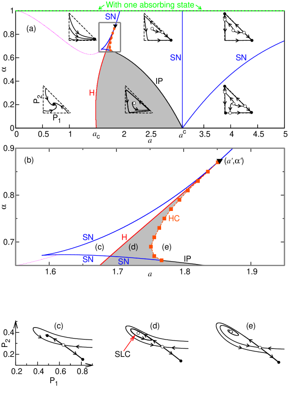
Figure 2: (a) Phase diagram with phases characterized by representative phase portraits. The triangles mark the border of the physically acceptable region $0\leqslant P_{1}\leqslant 1$, $0\leqslant P_{2}\leqslant 1$, and $0\leqslant P_{1}+P_{2}\leqslant 1$. Below (above) the dotted line [pink online] the stable fixed point is a spiral (node). The remaining lines represent bifurcations in the mean-field equations (3)-(5): Hopf (H) bifurcation (red online), saddle-node (SN) bifurcation (blue online) and infinite-period (IP) bifurcation (black). The squares indicate the homoclinic (HC) bifurcation line. The black triangle indicates the point $(a^{\prime},\alpha^{\prime})$ at which the HC, H and SN lines meet (see text for details). The dashed line (green online) on top of the panel (at $\alpha=1$) marks the parameter space region where there is a single absorbing state (but not necessarily a single attractor, see text for details). (b) Zoom of panel (a) displaying details near the homoclinic line. Panels (c), (d) and (e) show the phase portraits for the parameters marked in the panel (b), see also Fig. 4. SLC = stable limit cycle. There are stable limit cycles only in the grey regions.

Let $g_{i,j}$ be the transition rate from state $i$ to state $j$, given by (2), where $i\mbox{ and }j\in\{1,2,3\}$. In a mean-field approximation, this leads to the following equations:

$$\dot{P}_{1} = g_{3,1}(P_{3},P_{1})P_{3}-g_{1,2}(P_{1},P_{2})P_{1},$$ (3)

$$\dot{P}_{2} = g_{1,2}(P_{1},P_{2})P_{1}-g_{2,3}(P_{2},P_{3})P_{2},$$ (4)

$$\dot{P}_{3} = g_{2,3}(P_{2},P_{3})P_{2}-g_{3,1}(P_{3},P_{1})P_{3}.$$ (5)

This also coincides with the equations for a complete graph in the limit $N\to\infty$ with an inherent assumption that we can replace $N_{i}/N$ with $P_{i}$. Normalization ($P_{3}=1-P_{1}-P_{2}$) reduces these equations to a two-dimensional flow in the $(P_{1},P_{2})$ plane.

We start by analyzing the phase diagram of the mean-field equations (3)-(5) in the phase plane $(P_{1},P_{2})$, which is restricted to the triangle $0\leqslant P_{1}\leqslant 1$, $0\leqslant P_{2}\leqslant 1$, and $0\leqslant P_{1}+P_{2}\leqslant 1$. As shown in Fig. 2, the case of uniform oscillators (where the system has a perfect $C_{3}$ symmetry) shows two bifurcations as one increases $a$ on the line $\alpha=0$. First [12, 13], at $a=a_{c}=1.5$, a supercritical Hopf bifurcation occurs above which the symmetric fixed point $(P_{1}^{*},P_{2}^{*})=(1/3,1/3)$ loses stability and stable collective oscillations emerge [a limit cycle in the phase plane $(P_{1},P_{2})$]. Increasing $a$ further, the frequency of these global oscillations decreases continuously as the size of the limit cycle increases [32, 33]. For large values of $a$, the shape of the limit cycle becomes less circular, approaching the borders of the triangle, and global oscillations become highly anharmonic, with a finite fraction of the oscillators collectively spending a long time in each of the three states before “jumping” to the next state at a much shorter time scale. At $a=a^{c}\simeq 3.102$, three saddle-node (SN) bifurcations occur simultaneously at the limit cycle, corresponding to an infinite-period transition in which $C_{3}$ symmetry is broken (since three stable attractors are created) [34]. As noted previously [32], this second transition is somewhat artificial from the perspective of more realistic models, for which one expects (and observes) oscillators to lock at a coupling-independent frequency. However, it is very interesting from the perspective of nonequilibrium phase transitions of interacting particle systems, since it provides a spontaneous breaking of $C_{3}$ symmetry in the absence of any absorbing state [34] (as opposed to models with 3 absorbing states, like rock-paper-scissors games [35, 36, 37, 38, 39]).

For $\alpha>0$, $C_{3}$ symmetry is no longer present. In fact, even for arbitrarily small nonzero $\alpha$, the Hopf bifurcation is followed (as $a$ is increased) by an infinite-period transition which occurs due to a single SN bifurcation [as opposed to the triple SN for $\alpha=0$, see Fig. 2(a)]. Above this point, collective oscillations disappear because units tend to condensate in state 1, which is favored by the model nonuniformity [see Fig. 1]. Increasing $a$ further, another SN bifurcation occurs [Fig. 2(a)], in which a value of $P_{2}^{*}>1/3$ becomes a second stable fixed point of the model (i.e., state 2, which comes right after state 1, now can also attract the oscillators). Finally, for even larger values of $a$, a third SN bifurcation occurs and $P_{3}^{*}>1/3$ becomes a third attractor. With three attractors, the phase space is similar to that observed for $\alpha=0$.

Let us now address the stronger effects of the model nonuniformity. Consider first the leftmost portion of Fig. 2(a), i.e. for values of the coupling $a$ which are too small to yield sustained collective oscillations. In this regime, the only attractor is a stable spiral, which for $\alpha=0$ is symmetric: $(P_{1}^{*},P_{2}^{*})=(1/3,1/3)$. Increasing $\alpha$, this spiral moves towards larger values of $P_{1}^{*}$. Eventually, the imaginary part of its eigenvalues vanish and the fixed point becomes a node [dotted line (pink online) in Fig. 2a]. Only when $\alpha=1$ one reaches $P_{1}^{*}=1$, which is then (and only then) an absorbing state [Fig. 2a, upper dashed line (green online)].

Note that the infinite-period (IP) bifurcation line ends in the beginning of the SN and homoclinic bifurcation lines [Fig. 2(b)]. As we will see below, this happens because there is an intrinsic interdependence among these three bifurcations. An infinite-period bifurcation is just a SN bifurcation in which the saddle and the node are born at the limit cycle, whereas in the homoclinic bifurcation the limit cycle collides with a pre-existing saddle and becomes a homoclinic orbit. In both cases the period diverges at the bifurcation, though with different scaling regimes [30].

Now we turn to the main question of this article, namely, what happens if we start from a regime with collective oscillations (say, with $a>a_{c}$, $\alpha\gtrsim 0$) and increase the system nonuniformity? We will see that many scenarios exist, but all of them ultimately lead to the destruction of the limit cycle for some $\alpha\leqslant\alpha^{\prime}<1$ [Fig. 2(b)]. We consider first the simplest cases. If, on one hand, we fix a value of $a$ very close to $a_{c}$, the size of limit cycle will continuously decrease with increasing $\alpha$ to vanish in a supercritical Hopf bifurcation [H line (red online) in Figs. 2(a) and 2(b)]. If the fixed value of $a$ is sufficiently close to $a^{c}$, on the other hand, the limit cycle will be destroyed by increasing $\alpha$ via an infinite-period bifurcation [IP line in Figs. 2(a) and 2(b)].

There are intermediate values of $a$ for which the way to the annihilation of the limit cycle is more tortuous [Fig. 2(b)]. The key player to watch in these scenarios is a point $(a^{\prime},\alpha^{\prime})$ (with $a_{c}<a^{\prime}<a^{c}$ and $0<\alpha^{\prime}<1$) in parameter space where the Hopf bifurcation line ends [represented by a black triangle in the Figs. 2(a) and 2(b)]. For any $a\in(a_{c},a^{\prime})$, increasing $\alpha$ will lead to extinction of the limit cycle via a Hopf bifurcation [Figs. 2(a) and (b)]. For $a\lessapprox a^{\prime}$, the limit cycle is first destroyed by an infinite-period bifurcation, then emerges again through a homoclinic bifurcation, and finally disappears in a Hopf bifurcation [Fig. 2(b)]. There is also a small reentrance in the homoclinic bifurcation curve [Fig. 2(b)], so that for any value of $a$ in this short interval, the growth of $\alpha$ leads to destruction and recreation of limit cycle by two consecutive homoclinic bifurcations. Finally, for smaller values of $a$, a SN bifurcation leads to the phase portrait of the Fig. 2(d) before the limit cycle is annihilated by a Hopf bifurcation [Fig. 2(b)].

If we set $\alpha>\alpha^{\prime}$ and $a<a^{\prime}$, we will have only one stable node with $P_{1}^{*}\approx 1$ (remember that for $\alpha=1$ we have $P_{1}^{*}=1$, which corresponds to the absorbing state). Increasing $a$, there will be a first SN bifurcation at which a saddle is born with an unstable node (which quickly becomes a spiral) [Fig. 2(a)]. Further increases in $a$ will give rise to two additional SN bifurcations, as described above. After the third SN bifurcation, the system will have three attractors with a phase portrait of the same type as that of the figure 3(b). Importantly, besides the three saddle-node bifurcations mentioned, no other bifurcation occurs for $\alpha>\alpha^{\prime}$. In particular, we found no limit cycles for $\alpha^{\prime}<\alpha<1$, so that the nonuniformity alone can destroy collective oscillations, even in the absence of an absorbing state.

3.2 Complete graph simulations

Figure 3: Phase portraits and simulation results for a complete graph with $N=500$. Every 50 time units, the parameters of the model are changed so as to eliminate a stable fixed point of the model. (a) Phase diagram with labels to indicate the parameter-space places of the phase portraits (b)-(e) and arrows to show the order of the parameter-value jumps. (b) Phase portrait for $\alpha=0.2$ and $a=4$. The three samples of the simulations begin at the unstable fixed point close to triangle center, then each one converges to a different attractor owing to fluctuations. (c) Phase portrait for $\alpha=0.9$ and $a=4$. During the simulations, we change the parameter $\alpha$ to the value of this phase portrait. Thus, one of the attractors disappears, so the sample which was around one attractor converges to the stable fixed point of the attraction basin where this sample is now. Obviously, the other two samples continue around their attractor. (d) Phase portrait for $\alpha=0.9$ and $a=2.5$. Similarly to panel (c), another attractor disappears. Thus, the sample which was isolated converges to the remaining stable fixed point. (e) Phase portrait for $\alpha=0.2$ and $a=2.25$. Finally, the remaining stable fixed point disappears, so the three samples oscillate almost together (except for fluctuations). Panel (f) shows time series for simulated trajectories shown in panels (b), (c), (d), and (e), in chronological order. The false impression that the inequalities $0\leq P_{j}\leq 1$ are sometimes violated is caused by the thickness of the lines.

As mentioned in subsection 3.1, the mean-field calculations are exact for the complete graph in the thermodynamic limit. For completeness, we now study the effects of finite-size fluctuations. While we do not expect stable collective oscillations to appear for $\alpha\geqslant\alpha^{\prime}$, stochastic oscillations have been predicted to appear around (mean-field) stable spirals [40] in finite populations. Moreover, fluctuations become particularly prominent in systems with multistability, ultimately determining the attractor to which the system will converge.

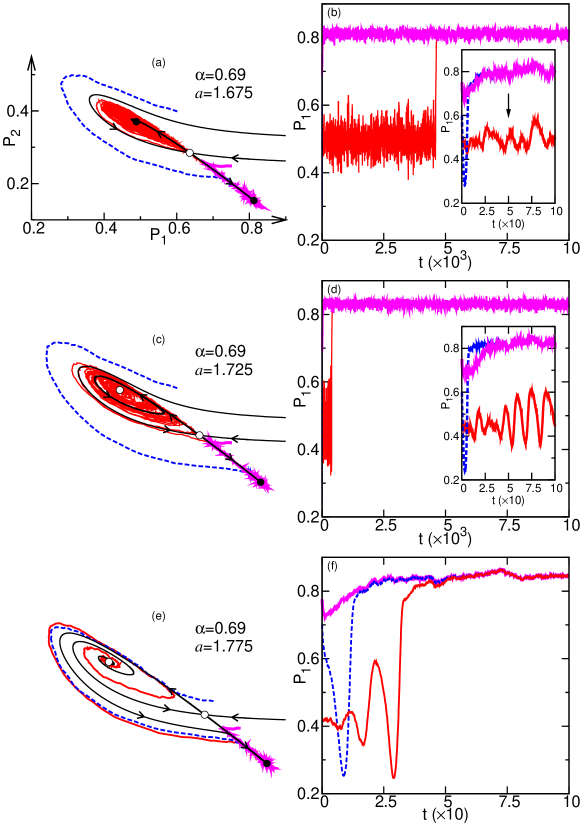
Figure 4: Phase portraits and simulation results for a complete graph with $N=20000$, see Fig. 2. (a) Phase portrait for $\alpha=0.69$ and $a=1.675$. There are two attractors: a node and a spiral (they are separated by a saddle). (c) Phase portrait for $\alpha=0.69$ and $a=1.725$. The spiral becomes unstable via a Hopf bifurcation and is surrounded by a stable limit cycle. (e) Phase portrait for $\alpha=0.69$ and $a=1.775$. After a homoclinic bifurcation, the limit cycle disappears. Panels (b), (d), and (f) show time series for simulated trajectories, respectively, shown in panels (a), (c), and (e), with examples of collective excitability (dashed, blue online) and stochastic oscillations [arrow in the inset of (b)].

First, let us deal with the effects of finite-size fluctuations in a scenario with multistability by starting the system near an unstable stationary solution at the intersection of the basins of attraction of the three stable solutions [Fig. 3(b)]. At point (b) in Fig. 3(a), tristability is revealed by the different fates of the system for three independent realizations of the same macroscopic initial condition.

Next, after each sample was already in its respective steady state, we have increased $\alpha$ discontinuously [(b)$\rightarrow$(c) in Fig. 3(a)] without interruption in the simulations in order to extinguish one of the attractors. Therefore, the sample which was around the newly extinct attractor converges to the stable solution of the new larger basin of attraction [while the other two samples are only slightly disturbed, see Fig. 3(c)].

Then, similarly to the previous case, we decrease $a$ discontinuously [(c)$\rightarrow$(d) in Fig. 3(a)] in order to suppress the attractor of the isolated sample, which is forced to converge to the remaining stable fixed point. At this stage, all three samples have the same behavior, apart from fluctuations [Fig. 3(d)].

Finally, we reduce $a$ and $\alpha$ discontinuously and simultaneously [(d)$\rightarrow$(e) in Fig. 3(a)] in order to eliminate the last stable fixed point. The three samples thereafter converge (at about the same time) to a stable limit cycle in which they oscillate almost together, apart from fluctuations [Fig. 3(e) and (f)]. Note that the process illustrated in Figure 3 does not close a cycle and is irreversible: no matter whether we change the control parameters to their initial values [i.e. (e)$\rightarrow$(b) in Fig. 3(a)], or we apply the reverse changes [(e)$\rightarrow$(d)$\rightarrow$(c)$\rightarrow$(b)], it is extremely unlikely that the system will return to its initial steady state [Figure 3(b)].

Now consider the phase diagram of Figure 2(b). In the far left (lower values of $a$) there is only one stable node. Increasing $a$, a SN bifurcation occurs in which a newly arisen node turns into a spiral after an extremely small increase in $a$. Thus, we get the phase portrait of the Figure 2(c), whose simulation results for a complete graph appear in Figures 4(a) and (b). Although the mean-field calculations predict that the spiral in Figures 2(c) and 4(a) is stable, even for large complete graphs ($N=20000$ in Figure 4) finite-size fluctuations eventually lead to system to the other (fixed point) attractor. However, before that happens, these fluctuations lead to stochastic oscillations around the spiral [40] [see arrow in the inset of Figure 4(b)].

Increasing $a$ further, the spiral loses stability in a Hopf bifurcation, giving rise to a stable limit cycle (SLC). We arrive then at the phase portrait shown in Figure 2(d), with simulation results for a complete graph shown in Figures 4(c) and (d). Again, while the mean-field calculations predict that the limit cycle in Figures 2(d) and 4(c) is stable, finite-size fluctuations lead the system to the other attractor in a considerably shorter time than in the previous case [Figs. 2(c), 4(a) and (b)].

Soon after the Hopf bifurcation, increasing $a$ leads to an increase in the size of the SLC, until it is finally destroyed by a homoclinic bifurcation [Fig. 2(b)]. Thus, we reach the phase portrait of the Figure 2(e), with the results of simulations of a complete graph shown in Figures 4(e) and (f). Now there is only one attractor in the system. As expected, if we start the system in the unstable spiral, there will be oscillations of increasing amplitude until the system reaches the stable steady state.

Note that the presence of the saddle in Figs. 2(c)-(e) sets the conditions for collective excitability [29]. If the system is initially in the stable node, perturbations that throw the system to a different point still within its basin of attraction can lead to qualitatively different relaxation processes. Small perturbations decay monotonically, whereas large perturbations will take the system further away from the fixed point before returning to it (because the system is required to go around the stable manifold of the saddle). This can be clearly seen in the simulations (compare the dashed and thick lines — blue and pink online, respectively — in Figure 4).

4 Concluding remarks

We have proposed a variant of the model by Wood et al. [12, 13] in which stochastic oscillators can become increasingly nonuniform as parameter $\alpha$ goes from 0 to 1. We have obtained the phase diagram of the mean-field version of the model in the $(a,\alpha)$ parameter plane. In addition to the previously reported phase transitions for $\alpha=0$ [12, 13, 34], we have obtained for $\alpha\neq 0$ several bifurcations in the mean-field equations of the model, including saddle-node, infinite period, Hopf and homoclinic. Collective excitability [29] has been shown to occur in some parameter regions, as confirmed by simulations of complete graphs. Simulations have also confirmed the overall predictions of the mean-field analysis, although the stability of some stable limit cycles and fixed points has failed to resist the effects of finite-size fluctuations.

In the regime in which the units are excitable elements, we did not find stable global oscillations for the particular choice of a nonlinear coupling defined by Eqs. 2, even in the complete graph. This topology is the one in which a synchronized solution would be most favorable, as shown in a number of previous reports [19, 12, 13, 40, 32, 33], which retrospectively justifies why we have not attempted to run simulations of the model in a hypercubic (or even small-world) topology. We have shown that, in the model of Wood et al. [12, 13], nonuniformity hinders the synchronization among the oscillators, while large enough nonuniformity and, consequently, the transformation of oscillatory units into excitable elements prevents the emergence of a synchronized stable state. It remains to be investigated whether this can be achieved with a different type of coupling.

Our results nonetheless raise some interesting questions which deserve further investigation. For any nonuniformity ($\alpha>0$) the transition to a synchronized state in the complete graph occurs in the absence of $C_{3}$ symmetry. Does the transition still occur in hypercubic lattices under these conditions [12]? If so, do the critical exponents depend on $\alpha$? Investigations in these directions would certainly be welcome.

5 Acknowledgments

VRVA and MC acknowledge financial support from CNPq, FACEPE, CAPES, FAPERJ and special programs PRONEX, PRONEM and INCEMAQ.

References

- Winfree [1967] A. T. Winfree, Biological rhythms and the behavior of populations of coupled oscillators, J. Theor. Biol. 16 (1967) 15–42.
- Kuramoto [1984] Y. Kuramoto (Ed.), Chemical Oscillations, Waves and Turbulence, Dover, Berlin, 1984.
- Strogatz and Stewart [1993] S. Strogatz, I. Stewart, Coupled oscillators and biological synchronization, Sci. Am. 269 (1993) 102–109.
- Strogatz [2000] S. H. Strogatz, From Kuramoto to Crawford: Exploring the onset of synchronization in populations of coupled oscillators, Physica D 143 (2000) 1–20.
- Huygens [1669] C. Huygens, Instructions concerning the use of pendulum-watches for finding the longitude at sea, Phil. Trans. R. Soc. Lond 4 (1669) 937–976.
- Strogatz [2004] S. H. Strogatz, Sync: How Order Emerges From Chaos In the Universe, Nature, and Daily Life, Hyperion, New York, 2004.
- Uhlhaas et al. [2009] P. J. Uhlhaas, G. Pipa, B. Lima, L. Melloni, S. Neuenschwander, D. Nikolić, W. Singer, Neural synchrony in cortical networks: history, concept and current status, Front. Integr. Neurosci. 3 (2009) 17.
- Koch [1999] C. Koch, Biophysics of Computation, Oxford University Press, New York, 1999.
- Ribeiro and Copelli [2008] T. L. Ribeiro, M. Copelli, Deterministic excitable media under Poisson drive: Power law responses, spiral waves and dynamic range, Phys. Rev. E 77 (2008) 051911.
- Erichsen and Brunnet [2008] R. Erichsen, Jr., L. G. Brunnet, Multistability in networks of Hindmarsh-Rose neurons, Phys. Rev. E 78 (2008) 061917.
- Agnes et al. [2010] E. J. Agnes, R. Erichsen, Jr., L. G. Brunnet, Synchronization regimes in a map-based model neural network, Physica A 389 (2010) 651–658.
- Wood et al. [2006a] K. Wood, C. Van den Broeck, R. Kawai, K. Lindenberg, Universality of synchrony: Critical behavior in a discrete model of stochastic phase-coupled oscillators, Phys. Rev. Lett. 96 (2006a) 145701.
- Wood et al. [2006b] K. Wood, C. Van den Broeck, R. Kawai, K. Lindenberg, Critical behavior and synchronization of discrete stochastic phase-coupled oscillators, Phys. Rev. E 74 (2006b) 031113.
- Risler et al. [2004] T. Risler, J. Prost, F. Jülicher, Universal critical behavior of noisy coupled oscillators, Phys. Rev. Lett. 93 (2004) 175702.
- Risler et al. [2005] T. Risler, J. Prost, F. Jülicher, Universal critical behavior of noisy coupled oscillators: A renormalization group study, Phys. Rev. E 72 (2005) 016130.
- Lindner et al. [2004] B. Lindner, J. García-Ojalvo, A. Neiman, L. Schimansky-Geier, Effects of noise in excitable systems, Phys. Rep. 392 (2004) 321–424.
- Anderson and May [1991] R. M. Anderson, R. M. May, Infectious Diseases of Humans: Dynamics and Control, Oxford University Press, Oxford, 1991.
- Liggett [1985] T. M. Liggett, Interacting Particles Systems, Springer-Verlag, 1985.
- Kuperman and Abramson [2001] M. Kuperman, G. Abramson, Small world effect in an epidemiological model, Phys. Rev. Lett. 86 (2001) 2909–2912.
- Gade and Sinha [2005] P. Gade, S. Sinha, Dynamic transitions in small world networks: Approach to equilibrium limit, Phys. Rev. E 72 (2005) 052903.
- Kinouchi and Copelli [2006] O. Kinouchi, M. Copelli, Optimal dynamical range of excitable networks at criticality, Nat. Phys. 2 (2006) 348–351.
- Rozenblit and Copelli [2011] F. Rozenblit, M. Copelli, Collective oscillations of excitable elements: order parameters, bistability and the role of stochasticity, J. Stat. Mech. (2011) P01012.
- Girvan et al. [2002] M. Girvan, D. S. Callaway, M. E. J. Newman, S. H. Strogatz, Simple model of epidemics with pathogen mutation, Phys. Rev. E 65 (2002) 031915.
- Joo and Lebowitz [2004] J. Joo, J. L. Lebowitz, Pair approximation of the stochastic susceptible-infected-recovered-susceptible epidemic model on the hypercubic lattice, Phys. Rev. E 70 (2004) 036114.
- Rozhnova and Nunes [2009a] G. Rozhnova, A. Nunes, Fluctuations and oscillations in a simple epidemic model, Phys. Rev. E 79 (2009a) 041922.
- Rozhnova and Nunes [2009b] G. Rozhnova, A. Nunes, SIRS dynamics on random networks: Simulations and analytical models, in: J. Zhou (Ed.), Complex Sciences, volume 4, Springer Berlin Heidelberg, 2009b, pp. 792–797. ArXiv:0812.1812v1 [q-bio.PE].
- Rozhnova and Nunes [2009c] G. Rozhnova, A. Nunes, Cluster approximations for infection dynamics on random networks, Phys. Rev. E 80 (2009c) 051915.
- Marro and Dickman [1999] J. Marro, R. Dickman, Nonequilibrium Phase Transition in Lattice Models, Cambridge University Press, Cambridge, 1999.
- Assis and Copelli [2009] V. R. V. Assis, M. Copelli, Discontinuous nonequilibrium phase transitions in a nonlinearly pulse-coupled excitable lattice model, Phys. Rev. E 80 (2009) 061105.
- Strogatz [1997] S. H. Strogatz, Nonlinear Dynamics and Chaos: with Applications to Physics, Biology, Chemistry and Engineering, Addison-Wesley, Reading, MA, 1997.
- Koch and Segev [1998] C. Koch, I. Segev (Eds.), Methods in Neuronal Modeling: From Ions to Networks, MIT Press, 2nd edition, 1998.
- Wood et al. [2007a] K. Wood, C. Van den Broeck, R. Kawai, K. Lindenberg, Effects of disorder on synchronization of discrete phase-coupled oscillators, Phys. Rev. E 75 (2007a) 041107.
- Wood et al. [2007b] K. Wood, C. Van den Broeck, R. Kawai, K. Lindenberg, Continuous and discontinuous phase transitions and partial synchronization in stochastic three-state oscillators, Phys. Rev. E 76 (2007b) 041132.
- Assis et al. [2011] V. R. V. Assis, M. Copelli, R. Dickman, An infinite-period phase transition versus nucleation in a stochastic model of collective oscillations, J. Stat. Mech. (2011) P09023.
- Tainaka [1988] K. Tainaka, Lattice model for the Lotka-Volterra system, J. Phys. Soc. Japan 57 (1988) 2588–2590.
- Tainaka [1989] K. Tainaka, Stationary pattern of vortices or strings in biological systems: Lattice version of the Lotka-Volterra model, Phys. Rev. Lett. 63 (1989) 2688–2691.
- Tainaka and Y. [1991] K. Tainaka, I. Y., Topological phase transition in biological ecosystems, Europhys. Lett. 15 (1991) 399–404.
- Tainaka [1994] K. Tainaka, Vortices and strings in a model ecosystem, Phys. Rev. E 50 (1994) 3401.
- Itoh and Tainaka [1994] Y. Itoh, K. Tainaka, Stochastic limit cycle with power-law spectrum, Phys. Lett. A 189 (1994) 37–42.
- Risau-Gusman and Abramson [2007] S. Risau-Gusman, G. Abramson, Bounding the quality of stochastic oscillations in populations models, Eur. Phys. J. B 60 (2007) 515–520.