Smoothness of Loewner Slits

Abstract

In this paper, we show that the chordal Loewner differential equation with $C^{\beta}$ driving function generates a $C^{\beta+\frac{1}{2}}$ slit for $\frac{1}{2}<\beta\leq 2$, except when $\beta=\frac{3}{2}$ the slit is only proved to be weakly $C^{1,1}$.

1 Introduction

The Loewner differential equation is a classical tool in complex analysis which has been successfully applied to various extremal problems, including the famous de Branges theorem (see [Bra]). In recent years, the Schramm-Loewner evolution (SLE) has been extensively studied by mathematicians and physicists. One can think of SLE as a random curve in the upper half-plane, which is generated via Loewner differential equation with a random driving function. In the meanwhile, some natural questions in the deterministic side of SLE are still open. In this paper, we investigate the smoothness of slits generated by $C^{\beta}$ driving functions.

Given a slit (definition in § 2) $\gamma\colon[0,T]\to\overline{\mathbb{H}}$ in the upper half-plane $\mathbb{H}=\{z\in\mathbb{C}\colon\text{Im}\,z>0\}$, the region $H_{t}:=\mathbb{H}\setminus\gamma([0,t])$ is simply connected for each $t$. There is a unique conformal map $g_{t}\colon H_{t}\to\mathbb{H}$ satisfying the hydrodynamic normalization

$$g_{t}(z)=z+\frac{a_{1}(t)}{z}+\frac{a_{2}(t)}{z^{2}}+\cdots$$

as $z\to\infty$. Figure 1 illustrates the situation. The coefficient $a_{1}(t)$ is called the half-plane capacity of the set $K_{t}=\gamma([0,t])$. See [RW] for a geometric interpretation of half-plane capacity and its relation to conformal radius, and see [LLN] for a probabilistic approach. Although it is not immediate from the definition, it is routine to show that $a_{1}(t)$ is a strictly increasing real-valued function with $a_{1}(0)=0$. If the slit is parametrized so that $a_{1}(t)=2t$, then $g_{t}(z)$ is differentiable in $t$ and satisfies the chordal Loewner differential equation

(1) $$\left\{\begin{aligned} \frac{\partial}{\partial t}g(t,z)&=\frac{2}{g(t,z)-\lambda(t)}\\ g(0,z)&=z\end{aligned}\right.$$

for $z\in H_{t}$, where $\lambda\colon[0,T]\to\mathbb{R}$ is a continuous function called the driving function of the slit. Moreover, $\lambda(t)=g_{t}(\gamma(t))$ is the image of the tip under the conformal map.

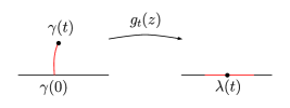
Figure 1: A slit $\gamma(t)$ and its driving function $\lambda(t)$ are related by a conformal map.

The foregoing procedure can be reversed. Suppose we are given some continuous function $\lambda\colon[0,T]\to\mathbb{R}$. For each $t\in[0,T]$, let $H_{t}$ be the set of points $z\in\mathbb{H}$ for which the solution of (1) is well-defined up to time $t$, i.e. $g(s,z)\not=\lambda(s)$ for $s\in[0,t]$. One can show that $H_{t}$ is a simply connected region and $z\mapsto g(t,z)$ maps $H_{t}$ conformally onto $\mathbb{H}$ and satisfies the hydrodynamic normalization. The set $K_{t}:=\mathbb{H}\setminus H_{t}$ is in general not a slit. Kufarev [Kuf] constructed an example, in the classical (radial) setting, for which a continuous driving function does not generate a slit. The example can also be found in [Dur, §3.4]. Even if the driving function is in $\text{Lip}(\frac{1}{2})$, also known as $\frac{1}{2}$-Holder continuous, the set $K_{t}$ may not be locally connected (see [MR] for an example).

Throughout this paper, we assume $\lambda\colon[0,T]\to\mathbb{R}$ is $\text{Lip}(\frac{1}{2})$, i.e.

$$\mbox{$\|\lambda\|_{\text{Lip}(\frac{1}{2})}$}:=\sup_{t_{1}\not=t_{2}\in[0,T]}\frac{\left|\lambda(t_{1})-\lambda(t_{1})\right|}{\left|t_{1}-t_{2}\right|^{\frac{1}{2}}}<\infty.$$

In 2005, Marshall and Rohde [MR] showed that there is an absolute constant $c_{0}>0$ so that for any $\lambda\colon[0,T]\to\mathbb{R}$ with $\mbox{$\|\lambda\|_{\text{Lip}(\frac{1}{2})}$}<c_{0}$, the Loewner equation (1) generates a quasi-slit in the upper half-plane $\mathbb{H}$ and the slit meets $\mathbb{R}$ non-tangentially. Lind [Lin] proved that all these statements hold for $c_{0}=4$, and this constant is the largest possible. On the other hand, in an unpublished paper [RTZ] Steffen Rohde, Huy Vo Tran and Michel Zinsmeister give a sufficient condition for the driving function to generate a rectifiable curve.

What more can we say if $\lambda\colon[0,T]\to\mathbb{R}$ is more regular (smooth) than $\text{Lip}(\frac{1}{2})$? In [Ale, page 59] , a Russian book published in 1976, it was proved that if $\lambda\colon[0,T]\to\mathbb{R}$ has bounded first derivative then its slit is $C^{1}$. (The original statement was a radial version. Here we formulate it in the chordal setting.) As of the writing of this paper and up to the author’s knowledge, it is the only result in the literature concerning the smoothness of a slit generated by a driving function more regular than $\text{Lip}(\frac{1}{2})$. Marshall and Rohde [MR] implicitly suggest the following.

Main Result (heuristic version).

$\lambda\in C^{\beta}\Rightarrow\gamma\in C^{\beta+\frac{1}{2}}$ for $\beta>\frac{1}{2}$.

In this paper, we will prove this statement for $\frac{1}{2}<\beta\leq 2$, except when $\beta=\frac{3}{2}$ the slit $\gamma$ is only proved to be weakly $C^{1,1}$. The precise statements are in Theorem 4.7, Theorem 5.2 and Theorem 6.2, corresponding to the cases $\beta\in(\frac{1}{2},1]$, $\beta\in(1,\frac{3}{2}]$ and $\beta\in(\frac{3}{2},2]$. One of the key ingredients of our method is the Lipschitz continuity (Theorem 3.3 below) of the map $\lambda\mapsto\gamma^{\lambda}$, which was only known to be continuous [LMR, Theorem 4.1]. Another ingredient is an integral representation of $\gamma^{\prime}(t)$, see Corollary 4.3.

Theorem 3.3 (Lipschitz continuity).

Suppose $\lambda_{1}$, $\lambda_{2}\colon[0,T]\to\mathbb{R}$ satisfy $\|\lambda_{j}\|_{\text{Lip}(\frac{1}{2})}\leq 1$ for $j=1$, 2. Then $\|\gamma^{\lambda_{1}}-\gamma^{\lambda_{2}}\|_{\infty}\leq c\,\|\lambda_{1}-\lambda_{2}\|_{\infty}$, where $c>0$ is an absolute constant.

There is another natural and interesting question which we won’t discuss in this paper but we mention it for the sake of completion. If we know a slit $\gamma$ is $C^{n}$, how smooth is its driving function? Earle and Epstein [EE] answered this question in 2001 for the radial case. Suppose $0\in\Omega\subseteq\mathbb{C}$ is a simply connected region and $\gamma\colon(0,T]\to\Omega$ is a slit avoiding the origin with base point $\gamma(0)\in\partial\Omega$. Let $R(t)$ be the conformal radius of $\Omega_{t}:=\Omega\setminus\gamma((0,T])$ with respect to the origin. Earle and Epstein showed that if $\gamma$ is $C^{n}$ regular on $(0,T]$ for some integer $n\geq 2$, then the radial capacity $a(t):=-\log R(t)$ is $C^{n-1}$ on (0,T]. Moreover, if the slit is reparametrized so that $a(t)=a(0)+t$, then its driving function $\lambda$ is $C^{n-1}$ on $(a(0),a(T)]$. See [EE] for the precise definitions and statements. In the same paper, it was also proved that real analytic slits generate real analytic driving functions.

Acknowledgement.

The author would like to thank Steffen Rohde for numerous inspiring discussions and suggestions. The author offers heartfelt thanks to Vo Huy Tran, Don Marshall, James Gill, Joan Lind, Matthew Badger and Christopher McMurdie for their suggestions and comments in the earlier versions of this paper.

2 Definitions, notations and preliminaries

General notation/convention.

2. $a(\varepsilon)\lesssim b(\varepsilon)$ means $a(\varepsilon)\leq Cb(\varepsilon)$ for some constant $C>0$ (independent of $\varepsilon$).

3. $a(\varepsilon)\asymp b(\varepsilon)$ means $a(\varepsilon)\lesssim b(\varepsilon)$ and $b(\varepsilon)\lesssim a(\varepsilon)$.

4. $a(\varepsilon)\simeq b(\varepsilon)$ as $\varepsilon\to 0$ if $\frac{a(\varepsilon)}{b(\varepsilon)}$ has a positive and finite limit.

5. In this paper, the lowercase $c$ is reserved to denote an absolute constant which may vary even in a single chain of equalities.

Definition.

A slit in $\mathbb{H}$ is a simple curve $\gamma\colon[0,T]\to\overline{\mathbb{H}}$ with $\gamma(0)\in\mathbb{R}$ and $\gamma(t)\in\mathbb{H}$ for $0<t\leq T$.

All driving functions $\lambda\colon[0,T]\to\mathbb{R}$ in this paper satisfy

$$\mbox{$\|\lambda\|_{\text{Lip}(\frac{1}{2})}$}:=\sup_{t_{1}\not=t_{2}\in[0,T]}\frac{\left|\lambda(t_{1})-\lambda(t_{1})\right|}{\left|t_{1}-t_{2}\right|^{\frac{1}{2}}}<4$$

(at least locally) and therefore generate slits by [MR] and [Lin]. We will use the following notations frequently.

Notation.

2. The $\text{Lip}(\frac{1}{2})$-norm of $\lambda\colon[0,T]\to\mathbb{R}$ is denoted by

   $$\|\lambda\|_{\text{Lip}(\frac{1}{2},[0,T])}:=\sup_{t_{1}\not=t_{2}\in[0,T]}\frac{\left|\lambda(t_{1})-\lambda(t_{2})\right|}{\left|t_{1}-t_{2}\right|^{\frac{1}{2}}}.$$

   Usually, we write $\|\lambda\|_{\text{Lip}(\frac{1}{2})}$ instead of $\|\lambda\|_{\text{Lip}(\frac{1}{2},[0,T])}$.

3. For positive integer $n\in\mathbb{N}$ and $0<\alpha\leq 1$, the $C^{n,\alpha}$-norm of $\lambda\colon[0,T]\to\mathbb{R}$ is

   $$\|\lambda\|_{C^{n,\alpha}}=\|\lambda\|_{C^{n,\alpha}([0,T])}:=\sum_{k=0}^{n}\sup_{t\in[0,T]}\left|\lambda^{(k)}(t)\right|+\sup_{t_{1}\not=t_{2}\in[0,T]}\frac{\left|\lambda^{(n)}(t_{1})-\lambda^{(n)}(t_{2})\right|}{\left|t_{1}-t_{2}\right|^{\alpha}}.$$

   For a slit $\gamma$, its $C^{n,\alpha}$-norm $\|\gamma\|_{C^{n,\alpha}}$ is defined similarly. If $\beta>1$ is not an integer, the notation $C^{\beta}$ refers to $C^{\left[\beta\right],\beta-\left[\beta\right]}$, where $\left[\beta\right]$ is the integer part of $\beta$. For example, $C^{\frac{3}{2}}$ is the same as $C^{1,\frac{1}{2}}$.

4. $\gamma^{\lambda}\colon[0,T]\to\overline{\mathbb{H}}$ denotes the slit generated by $\lambda\colon[0,T]\to\mathbb{R}$. When no confusion can occur, we write $\gamma$ instead of $\gamma^{\lambda}$ for the sake of notation. The base of $\gamma$ is $\gamma(0)=\lambda(0)\in\mathbb{R}$.

5. For each $t\in[0,T]$, $g_{t}\colon H_{t}\to\mathbb{H}$ denotes the (unique) conformal map from $H_{t}=\mathbb{H}\setminus\gamma([0,t])$ onto the upper half-plane $\mathbb{H}$ satisfying the normalization

   $$g_{t}(z)=z+\frac{a_{1}(t)}{z}+\cdots$$

   as $z\to\infty$. All slits in this paper are parametrized by half-plane capacity, i.e. $a_{1}(t)=2t$. Alternative notations such as $g(t,z)$ or $g^{\lambda}_{t}(z)$ may be used interchangeably.

6. $f_{t}\colon\mathbb{H}\to H_{t}$ is the inverse function of $g_{t}$, i.e. $g_{t}(f_{t}(z))=z$ for all $z\in\mathbb{H}$. We sometimes write $f(t,z)$ or $f_{t}^{\lambda}(z)$.

7. For $0\leq s<t\leq T$, we define $\gamma_{s}(t):=g_{s}(\gamma(t))-\lambda(s)$. To be flexible it may also be written as $\gamma(s,t)$ or $\gamma^{\lambda}_{s}(t)$. The normalized version of $\gamma(s,t)$ is $\tau(s,t):=\frac{\gamma(s,t)}{\sqrt{t-s}}$. Note that $\tau(s,t)=2i$ if and only if $\lambda$ is constant on $[s,t]$.

8. In §4, we introduce the notation

   $$L(s)=L^{\lambda}(s)=\int_{0}^{s}\left[\frac{1}{2}+\frac{2}{\tau(s-u,s)^{2}}\right]\frac{du}{u}$$

   and show that $\gamma^{\prime}(s)=\frac{i}{\sqrt{s}}\,e^{L(s)}$ under appropriate assumptions.

Definition.

2. We say that $\lambda\colon[0,T]\to\mathbb{R}$ satisfies the $\sigma$-Lip($\frac{1}{2}$) condition if $\sigma\geq 0$ and

   $$\left|\lambda(t_{1})-\lambda(t_{2})\right|\leq\sigma\left|t_{1}-t_{2}\right|^{\frac{1}{2}}$$

   for all $t_{1}$, $t_{2}\in[0,T]$.

3. We say that $\lambda\colon[0,T]\to\mathbb{R}$ satisfies the $(M,T,\delta)$-Lip($\frac{1}{2}+\delta$) condition if $\mbox{$\|\lambda\|_{\text{Lip}(\frac{1}{2})}$}\leq 1$ and

   $$\left|\lambda(t_{1})-\lambda(t_{2})\right|\leq M\left|t_{1}-t_{2}\right|^{\frac{1}{2}+\delta}$$

   for all $t_{1}$, $t_{2}\in[0,T]$, where $M$, $T$, $\delta>0$.

4. We say that $\lambda\colon[0,T]\to\mathbb{R}$ satisfies the $(M,T,n,\alpha)$-$C^{n,\alpha}$ condition if $\mbox{$\|\lambda\|_{\text{Lip}(\frac{1}{2})}$}\leq 1$, $\lambda\in C^{n,\alpha}$ on $[0,T]$ and $\|\lambda\|_{C^{n,\alpha}}\leq M$, where $n\in\mathbb{N}$, $0<\alpha\leq 1$ and $M>0$.

We will not consider $\text{Lip}(\frac{1}{2}+\delta)$ driving functions until §4. As a remark on terminologies, careful readers may see that in (i) we do not make explicit reference to $T$ but we do in (ii). This is because $\text{Lip}(\frac{1}{2}+\delta)$-norm is not invariant under Brownian scaling. The terminologies reflect that all quantitative estimates in §4 depend only on $M$, $T$ and $\delta$, while in §3 our estimates are mostly in terms of $\sigma$.

In this paper, we use the diagram in Figure 2 to represent a situation that $\gamma(t)$ and $\lambda(t)$ are related by the Loewner equation.

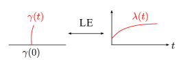
Figure 2: $\lambda(t)$ is the driving function of $\gamma(t)$.

For any continuous driving function $\lambda\colon[0,T]\to\mathbb{R}$, the solution $g_{t}(z)$ of (1) satisfies

(2) $$\log g_{t}^{\prime}(z) =-\int_{0}^{t}\frac{2}{[g_{u}(z)-\lambda(u)]^{2}}\,du$$

(3) $$g_{t}^{\prime\prime}(z) =4g_{t}^{\prime}(z)\int_{0}^{t}\frac{g_{u}^{\prime}(z)}{[g_{u}(z)-\lambda(u)]^{3}}\,du$$

for all $z\in H_{t}$. Equality (2) can be derived easily if we differentiate (1) with respect to $z$, which gives

$$\frac{\partial}{\partial t}g_{t}^{\prime}(z)=-\frac{2g_{t}^{\prime}(z)}{[g_{t}(z)-\lambda(t)]^{2}}.$$

To prove (3), we differentiate (2) with respect to $z$. We comment that (2) can be used to estimate the size of $\left|g_{s}^{\prime}(\gamma(s+\varepsilon))\right|$ as $\varepsilon\downarrow 0$, and this kind of estimates is crucial in our work as well as other SLE problems. Equality (3) will be useful if one wants to obtain second derivative estimates near the tip.

Equalities (2) and (3) hold for any continuous driving function $\lambda\colon[0,T]\to\mathbb{R}$. So far we haven’t made any smoothness assumption on $\lambda$. We are going to do it in the coming sections.

3 When $\lambda\in\text{Lip}(\frac{1}{2})$

We begin by stating some useful facts.

Fact.

Suppose $\lambda\colon[0,T]\to\mathbb{R}$ satisfies $\mbox{$\|\lambda\|_{\text{Lip}(\frac{1}{2})}$}<4$.

1. (Scaling property) If we define $\widetilde{\lambda}\colon[0,1]\to\mathbb{R}$ by $\widetilde{\lambda}(s):=\frac{1}{\sqrt{T}}\left[\lambda(sT)-\lambda(0)\right]$, then $\mbox{$\|\widetilde{\lambda}\|_{\text{Lip}(\frac{1}{2})}$}=\mbox{$\|\lambda\|_{\text{Lip}(\frac{1}{2})}$}$ and for all $s\in[0,1]$,

   $$\gamma^{\widetilde{\lambda}}(s)=\frac{1}{\sqrt{T}}\,\left[\gamma^{\lambda}(sT)-\gamma^{\lambda}(0)\right].$$

   For example, suppose a slit $\gamma$ is parametrized by half-plane capacity and $\lambda$ is the driving function of $\gamma$. The half-plane capacity reparametrization of the slit $3\gamma(t)$ is $\widetilde{\gamma}(t)=3\gamma(\frac{t}{9})$. The scaling property says that the driving function of $\widetilde{\gamma}$ is $\widetilde{\lambda}(t)=3\lambda(\frac{t}{9})$.

2. (Stationary property) For any $s\in(0,T)$, the time shift $\lambda_{s}\colon[0,T-s]\to\mathbb{R}$ of $\lambda$ is the function $\lambda_{s}(u):=\lambda(s+u)$. The corresponding slit is

   $$\gamma^{\lambda_{s}}(u)=g_{s}(\gamma(s+u)).$$

   See Figure 3 for an illustration.

3. For any $t\in[0,T]$,

   (4) $$\gamma^{\lambda}(t)=\lim_{y\downarrow 0}f_{t}(\lambda(t)+iy)=\lambda(t)-\int_{0}^{t}\frac{2}{\gamma(t-u,t)}\,du.$$

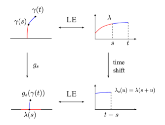
Figure 3: The stationary property states that the above diagram commutes.

The scaling property is extremely useful; in many situations it suffices to work only on the case $T=1$. The proofs of the scaling property and stationary property are elementary exercises. As we know from [MR] that $\gamma([0,t])$ is a slit (in particular, locally connected), it follows from Caratheodory continuity theorem (see, for example, [Pom, Theorem 2.1]) that the conformal map $f_{t}\colon\mathbb{H}\to H_{t}$ is continuous at the boundary point $\lambda(t)$. This proves the first equality in (4). The second equality is an immediate consequence of the Loewner differential equation (1) and the fundamental theorem of calculus applied to the function $u\mapsto g_{u}(\gamma(t))$ ($0\leq u\leq t$). The first equality in (4) is a non-trivial result for SLE curves, whose driving functions are random and almost surely not $\text{Lip}(\frac{1}{2})$ (see [RS], [LSW04]).

For $0\leq\sigma<4$, let $X_{\sigma}$ be the space of all (continuous) functions $\lambda\colon[0,1]\to\mathbb{R}$ satisfying $\lambda(0)=0$ and $\mbox{$\|\lambda\|_{\text{Lip}(\frac{1}{2})}$}\leq\sigma$. Under the supremum norm $\|\cdot\|_{\infty}$, the metric space $X_{\sigma}$ is compact. It is known [LMR, Theorem 4.1] that the map $X_{\sigma}\to\mathbb{H}$ defined by $\lambda\mapsto\gamma^{\lambda}(1)$ is continuous. It follows that $E_{\sigma}=\{\gamma^{\lambda}(1)\colon\lambda\in X_{\sigma}\}$ is a compact subset of $\mathbb{H}$.

By the scaling property,

$$\gamma^{\lambda}(t)\in\sqrt{t}\,E_{\sigma}$$

for any $0\leq t\leq 1$, $\lambda\in X_{\sigma}$, $0\leq\sigma<4$. On the other hand, it is easy to show (using compactness argument) that $E_{\sigma}$ shrinks to a singleton $\{2i\}$ as $\sigma\to 0$. Our first question is: at what rate does the diameter of $E_{\sigma}$ go to zero?

Lemma 3.1.

Suppose $\lambda\colon[0,1]\to\mathbb{R}$ satisfies the $\sigma$-Lip($\frac{1}{2}$) condition with $0\leq\sigma<4$ and $\lambda(0)=0$. Then

$$\left|\text{Re}\,\gamma^{\lambda}(1)\right|\leq\sigma\qquad\text{and}\qquad 4-\sigma^{2}\leq[\text{Im}\,\gamma^{\lambda}(1)]^{2}\leq 4.$$

In particular, $\text{diam}(E_{\sigma})\leq c\,\sigma$ for all $0\leq\sigma<4$, where $c>0$ is an absolute constant.

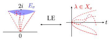
Figure 4: A sketch of the compact set $E_{\sigma}$ for $\sigma=1$. When $\sigma$ is close to zero, the set $E_{\sigma}$ becomes very thin by Lemma 3.1.

Proof.

Write $\gamma(t)=\gamma^{\lambda}(t)$ for the sake of notation. The estimate $\left|\text{Re}\,\gamma(1)\right|\leq\sigma$ follows from the simple observation that if $a\leq\lambda(t)\leq b$ for all $t\in[0,1]$, $z_{0}\in\mathbb{H}$ and $\text{Re}\,(z_{0})>b$ (respectively $\text{Re}\,(z_{0})<a$), then $g_{t}(z_{0})$ is defined and satisfies $\text{Re}\,g_{t}(z_{0})>b$ (respectively $\text{Re}\,g_{t}(z_{0})<a$) for all $t\in[0,1]$.

To estimate $\text{Im}\,\gamma(1)$, we use the fact that

$$\gamma(1)=\lim_{y\downarrow 0}h_{1}(\lambda(1)+iy),$$

where $h_{t}(z)$ is the solution to the initial value problem

(5) $$\left\{\begin{aligned} \dot{h}_{t}(z)&=-\frac{2}{h_{t}(z)-\xi(t)}\\ h_{0}(z)&=z\end{aligned}\right.$$

with $\xi(t):=\lambda(1-t)$. Fix any $y>0$ and write $h_{t}(\xi(0)+iy)=x_{t}+iy_{t}$ ($x_{t}$, $y_{t}\in\mathbb{R}$). Let $A_{t}=(x_{t}-\xi(t))^{2}$ and $B_{t}=y_{t}^{2}$. By scaling, or by our argument in the beginning of the proof, $A_{t}\leq\sigma^{2}t$ for all $0\leq t\leq 1$. Comparing the imaginary parts of (5), we have

$$\dot{B}_{t}=\frac{4B_{t}}{A_{t}+B_{t}}.$$

The obvious upper bound is $\dot{B}_{t}\leq 4$ and therefore $B_{1}\leq 4+y$, showing that $\text{Im}\,h_{t}(\lambda(1)+iy)\leq\sqrt{4+y}$. Letting $y\downarrow 0$ gives $\text{Im}\,\gamma(1)\leq 2$.

For the lower bound of $B_{1}$, we assume without loss of generality that $a:=4-\sigma^{2}>0$. (Otherwise, the lower bound is trivial.) Suppose for the sake of contradiction that $B_{t}<at$ for some $t\in[0,1)$. Let $T=\inf\{t\geq 0\colon B_{t}<at\}$. We have $0<T<1$, $B_{T}=aT$ and, for $0\leq t\leq T$,

$$\dot{B}_{t}=\frac{4B_{t}}{A_{t}+B_{t}}\geq\frac{4at}{\sigma^{2}t+at}=a.$$

This shows that $B_{T}\geq B_{0}+aT>aT$, which is a contradiction. We have proved that $B_{1}\geq 4-\sigma^{2}$. ∎

Consider the example $\lambda(t)=2\sqrt{\kappa}\,(1-\sqrt{1-t})$. When $0<\kappa<4$, this driving function satisfies the $\sigma$-Lip($\frac{1}{2}$) condition for $\sigma=2\sqrt{\kappa}$ and generates a logarithmic spiral with tip

$$\gamma(1)=\sqrt{\kappa}+i\sqrt{4-\kappa}=\frac{\sigma}{2}+i\sqrt{4-\frac{\sigma^{2}}{4}}.$$

(See [KNK] for the computation and [LMR] for a more conceptual approach.) This example together with Lemma 3.1 show

$$c_{1}\sigma\leq\text{diam}(E_{\sigma})\leq c_{2}\sigma.$$

for all $0<\sigma<4$, where $c_{1}$, $c_{2}>0$ are absolute constants.

The compactness of $E_{\sigma}$ has a simple geometric consequence. If $\lambda(0)=0$ and $\sigma=\mbox{$\|\lambda\|_{\text{Lip}(\frac{1}{2})}$}<4$, by scaling we see that $\gamma(t)\in\sqrt{t}E_{\sigma}$ and the slit $\gamma$ is contained in a cone whose angle depends on $\sigma$. If $\lambda\in\text{Lip}(\frac{1}{2}+\delta)$, one has $\gamma(t)\in\sqrt{t}E_{\sigma(t)}$ with $\sigma(t)\lesssim t^{\delta}$ as $t\to 0$. The slit grows vertically. See Figure 5.

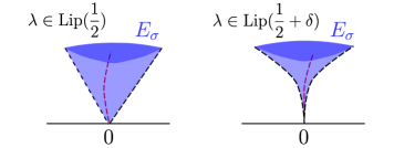
Figure 5: One main difference between slits of $\text{Lip}(\frac{1}{2})$ and $\text{Lip}(\frac{1}{2}+\delta)$ driving functions.

In §4, we will show that

$$\gamma^{\prime}(t)=\lim_{\varepsilon\downarrow 0}\frac{i}{\sqrt{\varepsilon}g_{t-\varepsilon}^{\prime}(\gamma(t))}=\lim_{\varepsilon\downarrow 0}\frac{i}{\sqrt{\varepsilon}g_{t}^{\prime}(\gamma(t+\varepsilon))}$$

under appropriate smoothness assumption on $\lambda$, and showing that $\left|g_{t}^{\prime}(\gamma(t+\varepsilon))\right|\simeq\varepsilon^{-\frac{1}{2}}$ as $\varepsilon\downarrow 0$ is more or less equivalent to showing that $\gamma^{\prime}(t)$ exists. Of course, in this section we are still in the $\text{Lip}(\frac{1}{2})$ case and do not expect $\gamma(t)$ to be differentiable. The next lemma says that $\left|g_{t-\varepsilon}^{\prime}(\gamma(t))\right|\asymp\varepsilon^{-\frac{1}{2}+O(\sigma)}$, with an error term in the exponent.

Lemma 3.2.

If $\lambda\colon[0,T]\to\mathbb{R}$ satisfies the $\sigma$-Lip($\frac{1}{2}$) condition for some $\sigma\in[0,1]$, then for any $0<s<t\leq T$,

$$\left(\frac{t}{t-s}\right)^{\frac{1}{2}-c\sigma}\leq\left|g_{s}^{\prime}(\gamma(t))\right|\leq\left(\frac{t}{t-s}\right)^{\frac{1}{2}+c\sigma},$$

where $c>0$ is an absolute constant.

Proof.

Without loss of generality, we assume $s=1$ and $\lambda(0)=0$. Let $w=\gamma(t)$. Then (2) gives

$$\log g^{\prime}_{1}(w)=\int_{0}^{1}-\frac{2}{\tau(u,t)^{2}}\,\frac{du}{t-u},$$

where $\tau(u,t)=\frac{g_{u}(w)-\lambda(u)}{\sqrt{t-u}}$ was defined in Notation (vi) in §2. If the driving function $\lambda$ is identically zero, $\tau^{\lambda}(u,t)$ becomes $\tau^{0}(u,t)\equiv 2i$ and the above equality reduces to

$$\frac{1}{2}\log\frac{t}{t-1}=\int_{0}^{1}\frac{1}{2}\,\frac{du}{t-u}.$$

Subtracting the two equalities gives

(6) $$\log g_{1}^{\prime}(w)-\frac{1}{2}\log\frac{t}{t-1}=-\int_{0}^{1}\left[\frac{1}{2}+\frac{2}{\tau(u,t)^{2}}\right]\frac{du}{t-u}.$$

By Lemma 3.1, $\left|\frac{1}{2}+\frac{2}{\tau(u,t)^{2}}\right|\leq c\sigma$, where $c>0$ is an absolute constant. Here we have implicitly used the condition $\sigma\leq 1$, which guarantees that $\tau(u,t)$ stays in a fixed compact set $E_{1}\subseteq\mathbb{H}$. The absolute constant $c$ in our last estimate is related to the derivative bound of the map $z\mapsto\frac{2}{z^{2}}$ on the compact set $E_{1}$.

Finally, equation (6) gives

$$\left|\log g^{\prime}_{1}(w)-\frac{1}{2}\log\frac{t}{t-1}\right|\leq\int_{0}^{1}\frac{c\,\sigma}{t-u}\,du=c\,\sigma\log\frac{t}{t-1}.$$

∎

Lemma 3.1 and the following Theorem 3.3 will serve as two fundamental tools for the rest of this paper.

Theorem 3.3 (Lipschitz continuity).

Suppose $\lambda$, $\widetilde{\lambda}\colon[0,T]\to\mathbb{R}$ satisfy the $\sigma$-Lip($\frac{1}{2}$) condition for $\sigma=1$. Then, $\left\|\gamma^{\lambda}-\gamma^{\widetilde{\lambda}}\right\|_{\infty}\leq c\,\left\|\lambda-\widetilde{\lambda}\right\|_{\infty}$, where $c>0$ is an absolute constant.

Fix any $T>0$. Let $\widetilde{X}_{\sigma}$ be the space of all (continuous) $\lambda\colon[0,T]\to\mathbb{R}$ with $\mbox{$\|\lambda\|_{\text{Lip}(\frac{1}{2})}$}\leq\sigma$. Recently, Joan Lind, Don Marshall and Steffen Rohde proved [LMR, Theorem 4.1] that the map $\lambda\mapsto\gamma^{\lambda}$ is a continuous map from $(\widetilde{X}_{\sigma},\|\cdot\|_{\infty})$ into $(C([0,T]),\|\cdot\|_{\infty})$ for every $0\leq\sigma<4$. Their proof uses the theory of quasi-conformal maps. When $\sigma\leq 1$, Theorem 3.3 says the map is Lipschitz continuous.

For $\sigma=1$, the slit $\gamma^{\lambda}$ of $\lambda\in X_{\sigma}$ is contained in the cone $V=\{z\in\mathbb{H}\colon\frac{\pi}{4}<\arg(z)<\frac{3\pi}{4}\}$. Theorem 3.3 remains true (with a larger absolute constant $c$) if the constant 1 is replaced by a slightly larger number where the slit is still contained in $V$. We do not know whether Theorem 3.3 holds for $\sigma=4-\varepsilon$ when $\varepsilon>0$ is small.

Proof.

By scaling we can assume $T=1$. Let $\varepsilon:=\sup_{0\leq t\leq 1}\left|\lambda(t)-\widetilde{\lambda}(t)\right|$. It also loses no generality to assume $\lambda(1)=\widetilde{\lambda}(1)$. (If not, translate one of the slits by $\lambda(1)-\widetilde{\lambda}(1)$, which has absolute value at most $\varepsilon$.) We extend $\lambda$ so that $\lambda(t)=\lambda(1)$ for all $t\geq 1$. Fix any small $\delta>0$. The tip $\gamma^{\lambda}(1+\delta)$ is equal to $h_{1}$, where $h_{t}\colon[0,1]\to\mathbb{C}$ is the solution of the backward Loewner differential equation

$$\left\{\begin{aligned} \partial_{t}h_{t}&=-\frac{2}{h_{t}-\xi(t)}\\ h_{0}&=\xi(0)+2i\sqrt{\delta}\end{aligned}\right.$$

and $\xi(t):=\lambda(1-t)$. Similarly, we extend $\widetilde{\lambda}$, define $\widetilde{\xi}(t)$, $\widetilde{h}_{t}$ and let $Y(t)=h_{t}-\widetilde{h}_{t}$. Note that $Y(1)=\gamma^{\lambda}(1+\delta)-\gamma^{\widetilde{\lambda}}(1+\delta)$ and $Y(0)=0$ since $\lambda(1)=\widetilde{\lambda}(1)$. By direct computation,

(7) $$\partial_{t}Y(t)=A(t)\left[Y(t)+\left(\widetilde{\xi}(t)-\xi(t)\right)\right],$$

where $A(t)=2(h_{t}-\xi(t))^{-1}(\widetilde{h}_{t}-\widetilde{\xi}(t))^{-1}$. We view (7) as a first order linear ODE in $Y(t)$ and solve it using the method of integrating factor. Let $\mu(t)=\exp\left(-\int_{0}^{t}A(s)\,ds\right)$. One has $\frac{d}{dt}\left[\mu(t)Y(t)\right]=\mu(t)A(t)\left(\widetilde{\xi}(t)-\xi(t)\right)$ and

$$Y(1)=\int_{0}^{1}\frac{\mu(s)}{\mu(1)}A(s)\left(\widetilde{\xi}(s)-\xi(s)\right)\,ds.$$

We know $\left|\widetilde{\xi}(s)-\xi(s)\right|\leq\varepsilon$ for all $s\in[0,1]$. To complete the proof, it remains to estimate the size of the integrating factor $\mu(t)$.

Notice that $A(t)\in\frac{1}{t+\delta}K$ for all $t\in[0,1]$, where

$$K=\left\{\frac{2}{z_{1}z_{2}}\colon z_{1},z_{2}\in E_{1}\right\}$$

and $E_{1}$ is the compact set defined right before Lemma 3.1 (see Figure 4). For convenience of the readers, we recall the definition

$$E_{1}:=\left\{\gamma^{\lambda}(1)\colon\lambda(0)=0\text{ and }\|\lambda\|_{\text{Lip}(\frac{1}{2},[0,1])}\leq 1\right\}.$$

By Lemma 3.1, $K$ is contained in the left half-plane $\{z\in\mathbb{C}\colon\text{Re}\,(z)<0\}$. Let

$$\beta=\inf\{-\text{Re}\,(z)\colon z\in K\}>0.$$

Since $A(t)\in\frac{1}{t+\delta}K$, we have $-\text{Re}\,A(t)\geq\frac{\beta}{t+\delta}$ for all $t\in[0,1]$. For any $s\in[0,1]$,

$$\frac{\mu(s)}{\mu(1)}=\exp\left[\int_{s}^{1}A(u)\,du\right]\qquad\text{and}\qquad\left|\frac{\mu(s)}{\mu(1)}\right|\leq(s+\delta)^{\beta}.$$

Finally,

$$\left|\gamma^{\lambda}(1+\delta)-\gamma^{\widetilde{\lambda}}(1+\delta)\right|=\left|Y(1)\right|\leq\varepsilon\int_{0}^{1}\left|\frac{\mu(s)}{\mu(1)}\right|\cdot\left|A(s)\right|\,ds\leq c\,\varepsilon\int_{0}^{1}(s+\delta)^{-1+\beta}\,ds.$$

where $c=\sup_{z\in K}\left|z\right|<\infty$ is an absolute constant. The result follows by letting $\delta\to 0$. ∎

4 When $\lambda\in\text{Lip}(\frac{1}{2}+\delta)$ with $0<\delta\leq\frac{1}{2}$

In this section, $\lambda\colon[0,T]\to\mathbb{R}$ satisfies the $(M,T,\delta)$-Lip($\frac{1}{2}+\delta$) condition, i.e. $\mbox{$\|\lambda\|_{\text{Lip}(\frac{1}{2})}$}\leq 1$ and

$$\left|\lambda(t_{1})-\lambda(t_{2})\right|\leq M\left|t_{1}-t_{2}\right|^{\frac{1}{2}+\delta}$$

for all $t_{1}$, $t_{2}\in[0,T]$, where $M$, $T$, $\delta>0$. The extra smoothness allows us to improve the exponent in Lemma 3.2.

Lemma 4.1.

If $\lambda\colon[0,T]\to\mathbb{R}$ satisfies the $(M,T,\delta)$-Lip($\frac{1}{2}+\delta$) condition for some $0<\delta\leq\frac{1}{2}$, then for any $0<s<t\leq T$,

(8) $$\frac{1}{C}\leq\sqrt{\frac{t-s}{t}}\left|g_{s}^{\prime}(\gamma(t))\right|\leq C,$$

where $C=C(M,T,\delta)>0$. Moreover, for all $s\in(0,T)$, the limit

$$\lim_{\varepsilon\downarrow 0}\sqrt{\varepsilon}g_{s}^{\prime}(\gamma(s+\varepsilon))=\sqrt{s}\exp\left\{-\int_{0}^{s}\left[\frac{1}{2u}+\frac{2}{\gamma(s-u,s)^{2}}\right]du\right\}$$

exists and is nonzero.

Proof.

As in the proof of Lemma 3.2,

$$\log g_{s}^{\prime}(\gamma(t))-\frac{1}{2}\log\frac{t}{t-s}=-\int_{0}^{s}\left[\frac{1}{2}+\frac{2}{\tau(u,t)^{2}}\right]\frac{du}{t-u}.$$

The $(M,T,\delta)$-Lip($\frac{1}{2}+\delta$) condition implies $\|\lambda\|_{\text{Lip}(\frac{1}{2},[u,t])}\leq M(t-u)^{\delta}$. Lemma 3.1 gives an estimate of our integral kernel:

$$\left|\frac{1}{2}+\frac{2}{\tau(u,t)^{2}}\right|\leq c\left|\tau(u,t)-2i\right|\leq cM(t-u)^{\delta}$$

for some absolute constant $c>0$. (Again, we have implicitly used the condition $\mbox{$\|\lambda\|_{\text{Lip}(\frac{1}{2})}$}\leq 1$, which guarantees that $\tau^{\lambda}(u,t)$ stays in a fixed compact set $E_{1}\subseteq\mathbb{H}$.) We have proved

$$\left|\log g_{s}^{\prime}(\gamma(t))-\frac{1}{2}\log\frac{t}{t-s}\right|\leq cM\int_{0}^{s}(t-u)^{\delta-1}\,du=\frac{cM}{\delta}\left(t^{\delta}-(t-s)^{\delta}\right)\leq\frac{cMs^{\delta}}{\delta}$$

and (8) follows. Taking $t=s+\varepsilon$ with $\varepsilon>0$ gives

$$\log\frac{\sqrt{\varepsilon}g_{s}^{\prime}(\gamma(s+\varepsilon))}{\sqrt{s+\varepsilon}}=-\int_{0}^{s}\left[\frac{1}{2}+\frac{2}{\tau(u,s+\varepsilon)^{2}}\right]\frac{du}{s+\varepsilon-u}.$$

The existence of $\lim_{\varepsilon\downarrow 0}\sqrt{\varepsilon}g_{s}^{\prime}(\gamma(s+\varepsilon))$ follows from the Lebesgue dominated convergence theorem. ∎

Lemma 4.2.

Let $\lambda_{1}$, $\lambda_{2}\colon[0,T]\to\mathbb{R}$ satisfy the $(M,T,\delta)$-Lip($\frac{1}{2}+\delta$) condition for some $0<\delta\leq\frac{1}{2}$. Suppose $\lambda_{1}=\lambda_{2}$ on $[0,s]$ for some $s\in(0,T)$. Then, for any $\varepsilon\in(0,T-s]$,

$$\left|\gamma^{\lambda_{1}}(s+\varepsilon)-\gamma^{\lambda_{2}}(s+\varepsilon)\right|\leq C\varepsilon^{1+\delta},$$

where $C=C(M,T,\delta,s)>0$.

Proof.

With $M$, $T$, $\delta$ fixed, let $X$ be the space of all functions $\lambda\colon[0,T]\to\mathbb{R}$ satisfying the $(M,T,\delta)$-Lip($\frac{1}{2}+\delta$) condition and $\lambda=\lambda_{1}$ on $[0,s]$. For each $\varepsilon\in(0,T-s]$, consider the compact set

$$K_{\varepsilon}=\left\{\gamma^{\lambda}(s+\varepsilon)\in\mathbb{H}\colon\lambda\in X\right\}.$$

It suffices to show $\text{diam}(K_{\varepsilon})\leq C\varepsilon^{1+\delta}$. Let $g_{s}=g_{s}^{\lambda_{j}}$ be the hydrodynamically normalized conformal map from $\mathbb{H}\setminus\gamma^{\lambda_{j}}([0,s])$ onto $\mathbb{H}$, and let $f_{s}=g_{s}^{-1}$. Note that

$$\text{diam}(K_{\varepsilon})\leq\text{diam}(g_{s}(K_{\varepsilon}))\cdot\sup_{z\in E}\left|f_{s}^{\prime}(z)\right|,$$

where $E$ is the convex hull of $g_{s}(K_{\varepsilon})$. By Lemma 3.1, $\text{diam}(g_{s}(K_{\varepsilon}))\leq cM\varepsilon^{\frac{1}{2}+\delta}$. On the other hand, Lemma 4.1 implies

(9) $$\sup_{z\in g_{s}(K_{\varepsilon})}\left|f_{s}^{\prime}(z)\right|\leq C\sqrt{\varepsilon},$$

where $C=C(M,T,\delta,s)>0$ does not depend on $\varepsilon$. If we replace $g_{s}(K_{\varepsilon})$ by its convex hull, the supremum in (9) can only increase by a bounded factor, by Koebe distortion theorem (see [Pom]) and the fact that the hyperbolic diameter of $g_{s}({K_{\varepsilon}})$ is bounded above by some absolute constant $c_{1}$. Actually, we can take $c_{1}$ to be the hyperbolic diameter of the set $E_{1}$ in Figure 4. ∎

Corollary 4.3.

Suppose $\lambda\colon[0,T]\to\mathbb{R}$ satisfies the $(M,T,\delta)$-Lip($\frac{1}{2}+\delta$) condition for some $0<\delta\leq\frac{1}{2}$, then $\gamma=\gamma^{\lambda}$ is differentiable on $(0,T)$ and

(10) $$\gamma^{\prime}(s)=\frac{i}{\sqrt{s}}\exp\left\{\int_{0}^{s}\left[\frac{1}{2u}+\frac{2}{\gamma(s-u,s)^{2}}\right]du\right\}$$

for all $s\in(0,T)$. At $s=T$, the left derivative $\gamma_{-}^{\prime}(T)$ exists and is given by the same formula.

Proof.

It suffices to show that the right derivative $\gamma_{+}^{\prime}(s)$ exists for $s\in(0,T)$ and is given by (10). (Using Theorem 3.3, it is not hard to see that (10) is continuous in $s$, and it is an exercise to show that any right differentiable function on an open interval with continuous right derivative is in fact differentiable. A proof of this elementary fact can be found in [Law, Lemma 4.3].)

Fix any $s\in(0,T)$. We may assume without loss of generality that $\lambda(t)=\lambda(s)$ for all $t\in[s,T]$, because modifying $\lambda$ this way does not change the right derivative $\gamma_{+}^{\prime}(s)$, by Lemma 4.2. We have $\gamma(s+\varepsilon)=f_{s}(\lambda(s)+2i\sqrt{\varepsilon})$ and therefore

$$\gamma(s+\varepsilon)-\gamma(s)=\int_{0}^{\varepsilon}\frac{if_{s}^{\prime}(\lambda(s)+2i\sqrt{u})}{\sqrt{u}}\,du$$

for all $\varepsilon\in(0,T-s]$. By Lemma 4.1, the integrand is continuous at $u=0$. It follows that $\gamma_{+}^{\prime}(s)$ exists and is given by

$$\gamma_{+}^{\prime}(s)=\lim_{\varepsilon\downarrow 0}\frac{if_{s}^{\prime}(\lambda(s)+2i\sqrt{\varepsilon})}{\sqrt{\varepsilon}}=\frac{i}{\sqrt{s}}\exp\left\{\int_{0}^{s}\left[\frac{1}{2u}+\frac{2}{\gamma(s-u,s)^{2}}\right]du\right\}.$$

∎

By formula (10), proving the smoothness of $\gamma$ is equivalent to proving the smoothness of the integral, which we call $L(s)$ from now on.

Notation.

Let

$$L(s)=L^{\lambda}(s)=\int_{0}^{s}\left[\frac{1}{2u}+\frac{2}{\gamma(s-u,s)^{2}}\right]du.$$

This integral makes sense provided that $\lambda\colon[0,T]\to\mathbb{R}$ satisfies the $(M,T,\delta)$-Lip($\frac{1}{2}+\delta$) condition for some $0<\delta\leq\frac{1}{2}$. In the coming sections, when we impose more regularity assumptions on $\lambda$, we will keep this notation.

In the proof of Lemma 4.1, we have implicitly proved an upper bound of $\left|L(s)\right|$. By (10), controlling the size of $\left|L(s)\right|$ gives an upper bound of $\left|\gamma^{\prime}(s)-\frac{i}{\sqrt{s}}\right|$. This estimate will be useful later and we now explicitly state it.

Lemma 4.4.

Under the $(M,T,\delta)$-Lip($\frac{1}{2}+\delta$) condition with $0<\delta\leq\frac{1}{2}$,

$$\left|L(s)\right|\leq\frac{cMs^{\delta}}{\delta}$$

for all $s\in[0,T]$, where $c>0$ is an absolute constant.

We will show that $L\in\text{Lip}(\delta)$. For any $s\in(0,T)$ and $\varepsilon\in[0,T-s]$,

(11) $$L(s+\varepsilon)-L(s)= \int_{0}^{s}\left[\frac{2}{\tau(s+\varepsilon-u,s+\varepsilon)^{2}}-\frac{2}{\tau(s-u,s)^{2}}\right]\frac{du}{u}+$$

$$\int_{s}^{s+\varepsilon}\left[\frac{1}{2}+\frac{2}{\tau(s+\varepsilon-u,s+\varepsilon)^{2}}\right]\frac{du}{u}.$$

Since $\|\lambda\|_{\text{Lip}(\frac{1}{2},[a,b])}\leq M(b-a)^{\delta}$, Lemma 3.1 gives $\left|\tau(s+\varepsilon-u,s+\varepsilon)-2i\right|\leq cMu^{\delta}$ and therefore

(12) $$\int_{s}^{s+\varepsilon}\left|\frac{1}{2}+\frac{2}{\tau(s+\varepsilon-u,s+\varepsilon)^{2}}\right|\,\frac{du}{u}\leq\int_{s}^{s+\varepsilon}cMu^{\delta-1}\,du\leq\frac{cM}{\delta}\varepsilon^{\delta}.$$

The second integral in (11) is under control. The first integral can be estimated using the quantity

(13) $$\omega(s,u,\varepsilon):=\sup_{0\leq v\leq u}\left|\lambda(s+\varepsilon-v)-\lambda(s+\varepsilon-u)-\lambda(s-v)+\lambda(s-u)\right|.$$

Note that $\omega(s,u,\varepsilon)$ can be expressed as $\|\lambda_{1}-\lambda_{2}\|_{\infty}$, where $\lambda_{1}$, $\lambda_{2}\colon[0,u]\to\mathbb{R}$ are driving functions whose tips are $\gamma(s+\varepsilon-u,s+\varepsilon)$ and $\gamma(s-u,s)$. Theorem 3.3 implies

$$\left|\gamma(s+\varepsilon-u,s+\varepsilon)-\gamma(s-u,s)\right|\leq c\,\omega(s,u,\varepsilon)$$

for some absolute constant $c>0$. This gives an estimate of the first integral in (11). We have proved the following lemma.

Lemma 4.5.

If $\lambda\colon[0,T]\to\mathbb{R}$ satisfies the $(M,T,\delta)$-Lip($\frac{1}{2}+\delta$) condition for some $0<\delta\leq\frac{1}{2}$, then for any $0\leq s<s+\varepsilon\leq T$,

(14) $$\left|L(s+\varepsilon)-L(s)\right| \leq c\int_{0}^{s}u^{-\frac{3}{2}}\,\omega(s,u,\varepsilon)\,du+\frac{cM}{\delta}\left[(s+\varepsilon)^{\delta}-s^{\delta}\right]$$

$$\leq c\int_{0}^{s}u^{-\frac{3}{2}}\,\omega(s,u,\varepsilon)\,du+\frac{cM\varepsilon^{\delta}}{\delta},$$

where $c>0$ is an absolute constant $\omega(s,u,\varepsilon)$ is defined in (13).

The first inequality in (14) will be used in §5, and we use the second estimate in this section. When $\delta=\frac{1}{2}$, we will see soon (14) gives $\left|L(s+\varepsilon)-L(s)\right|=O(\sqrt{\varepsilon})$ as $\varepsilon\downarrow 0$. We achieve this by controlling the size of $\omega(s,u,\varepsilon)$. The estimate depends on the regularity of $\lambda$. In this section, $\lambda$ is only $\text{Lip}(\frac{1}{2}+\delta)$, the following estimate of $\omega(s,u,\varepsilon)$ is what we should expect and will be improved in §5 under the assumption $\lambda\in C^{1,\delta}$.

Lemma 4.6.

Let $\lambda\colon[0,T]\to\mathbb{R}$ satisfy the $(M,T,\delta)$-Lip($\frac{1}{2}+\delta$) condition. For any $0\leq s<s+\varepsilon\leq T$ and $0<u<s$,

$$\omega(s,u,\varepsilon)\leq\begin{cases}2Mu^{\frac{1}{2}+\delta},&u\leq\varepsilon\\ 2M\varepsilon^{\frac{1}{2}+\delta},&u\geq\varepsilon\\ \end{cases}$$

and $\left|L(s+\varepsilon)-L(s)\right|\leq C\varepsilon^{\delta}$, where $C=C(M,T,\delta)>0$.

Proof.

When $u\leq\varepsilon$,

$$\left|\lambda(s+\varepsilon-v)-\lambda(s+\varepsilon-u)-\lambda(s-v)+\lambda(s-u)\right|$$

$$\leq \left|\lambda(s+\varepsilon-v)-\lambda(s+\varepsilon-u)\right|+\left|\lambda(s-v)-\lambda(s-u)\right|$$

$$\leq 2Mu^{\frac{1}{2}+\delta}$$

for any $0\leq v\leq u$. When $u\geq\varepsilon$, we rearrange terms as

$$\left|\lambda(s+\varepsilon-v)-\lambda(s+\varepsilon-u)-\lambda(s-v)+\lambda(s-u)\right|$$

$$\leq \left|\lambda(s+\varepsilon-v)-\lambda(s-v)\right|+\left|\lambda(s+\varepsilon-u)-\lambda(s-u)\right|$$

$$\leq 2M\varepsilon^{\frac{1}{2}+\delta}$$

for any $0\leq v\leq u$. We have proved the desired estimates of $\omega(s,u,\varepsilon)$.

To prove $\left|L(s+\varepsilon)-L(s)\right|\leq C\varepsilon^{\delta}$, we split the integral in (14):

$$\left|\int_{0}^{s}u^{-\frac{3}{2}}\,\omega(s,u,\varepsilon)\,du\right|\leq\int_{0}^{\varepsilon}2Mu^{-1+\delta}\,du+\int_{\varepsilon}^{s}2Mu^{-\frac{3}{2}}\varepsilon^{\frac{1}{2}+\delta}\,du\leq C\varepsilon^{\delta}$$

∎

We have all the ingredients for proving our first main result.

Theorem 4.7.

Let $\lambda\colon[0,T]\to\mathbb{R}$ be such that

$$\left|\lambda(t_{1})-\lambda(t_{2})\right|\leq M\left|t_{1}-t_{2}\right|^{\frac{1}{2}+\delta}$$

for all $t_{1}$, $t_{2}\in[0,T]$, where $M>0$ and $\delta\in(0,\frac{1}{2}]$ are constants. Then

1. $\Gamma(t):=\gamma(t^{2})$ is $C^{1,\delta}$ regular on $[0,\sqrt{T}]$; and

2. the slit $\gamma(t)$ grows vertically at $t=0$.

With an extra assumption that $\mbox{$\|\lambda\|_{\text{Lip}(\frac{1}{2})}$}\leq 1$, these statements are quantitative:

(15) $$\|\Gamma\|_{C^{1,\delta}([0,T])}\leq N\qquad\text{and}\qquad\inf_{t\in[0,T]}\left|\Gamma^{\prime}(t)\right|\geq\frac{1}{N},$$

where $N=N(M,T,\delta)>0$ depends only on $M$, $T$ and $\delta$. Furthermore,

(16) $$\left|\Gamma^{\prime}(t)-2i\right|\leq N\,t^{2\delta}\qquad(0<t\leq\sqrt{T}).$$

Proof of Theorem 4.7.

We first assume $\mbox{$\|\lambda\|_{\text{Lip}(\frac{1}{2})}$}\leq 1$. By Corollary 4.3, $\Gamma(t)=\gamma(t^{2})$ is differentiable and $\Gamma^{\prime}(t)=2ie^{L(t^{2})}$. With this formula of $\Gamma^{\prime}(t)$, we claim that $\Gamma^{\prime}(t)$ is $\text{Lip}(\delta)$. To see this, we first note from Lemma 4.4 that $\sup_{0\leq t\leq\sqrt{T}}\left|L(t^{2})\right|\leq R$ for some constant $R=\frac{cMT^{\delta}}{\delta}$ depending only on $M$, $T$ and $\delta$. This tells us

$$\left|\Gamma^{\prime}(t_{1})-\Gamma^{\prime}(t_{2})\right|\leq 2\left(\sup_{\left|z\right|\leq R}\left|e^{z}\right|\right)\left|L(t_{1}^{2})-L(t_{2}^{2})\right|\leq C\left|t_{1}-t_{2}\right|^{\delta}$$

for some $C=C(M,T,\delta)>0$ by Lemma 4.6. This proves (a). The estimates (15) and (16) follow from Lemma 4.4 and other estimates we have proved. For example,

$$\left|\Gamma^{\prime}(t)\right|=2\left|e^{L(t^{2})}\right|=2e^{\text{Re}\,L(t^{2})}\geq 2e^{-R}$$

and (16) can be derived from

$$\left|\Gamma^{\prime}(t)-2i\right|=2\left|e^{L(t^{2})}-1\right|\leq 2\left(\sup_{\left|z\right|\leq R}\left|e^{z}\right|\right)\left|L(t^{2})\right|.$$

If $\mbox{$\|\lambda\|_{\text{Lip}(\frac{1}{2})}$}>1$, we pick a partition $0=t_{0}<t_{1}<\cdots<t_{n}=T$ for which $M(t_{j+2}-t_{j})^{\delta}<1$ for all $j=0$, 1, …, $n-2$. This guarantees that $\|\lambda\|_{\text{Lip}(\frac{1}{2},[t_{j},t_{j+2}])}<1$ for all $j$. It suffices to show

1. $\Gamma(t)=\gamma(t^{2})$ is $C^{1,\delta}$ regular on $[t_{0},t_{2}]$; and

2. $\gamma(t)$ is $C^{1,\delta}$ regular on $[t_{j},t_{j+2}]$ for $j=1$, 2, …, $n-2$.

(i) follows from the argument of the previous paragraph, since we are back to the case $\mbox{$\|\lambda\|_{\text{Lip}(\frac{1}{2})}$}\leq 1$. To show (ii), we pick $\varepsilon>0$ for which $M(t_{j+2}-t_{j}+\varepsilon)^{\delta}\leq 1$. Again, by our earlier argument for the case $\mbox{$\|\lambda\|_{\text{Lip}(\frac{1}{2})}$}\leq 1$, the function

$$u\mapsto\gamma(t_{j}-\varepsilon,t_{j}+u)$$

is $C^{1,\delta}$ regular on $[0,t_{t+2}-t_{j}]$, and therefore

$$u\mapsto\gamma(t_{j}+u)=f_{t_{j}-\varepsilon}(\lambda(t_{j}-\varepsilon)+\gamma(t_{j}-\varepsilon,t_{j}+u))$$

is also $C^{1,\delta}$ regular on $[0,t_{j+2}-t_{j}]$. ∎

5 When $\lambda\in C^{1,\delta}$ with $0<\delta\leq\frac{1}{2}$

In this section, our driving function $\lambda\colon[0,T]\to\mathbb{R}$ satisfies the $(M,T,1,\delta)$-$C^{1,\delta}$ condition with $0<\delta\leq\frac{1}{2}$. That is to say, $\mbox{$\|\lambda\|_{\text{Lip}(\frac{1}{2})}$}\leq 1$, $\lambda\in C^{1}([0,T])$ and

$$\|\lambda\|_{C^{1,\delta}}=\sup_{t\in[0,T]}\left|\lambda(t)\right|+\sup_{t\in[0,T]}\left|\lambda^{\prime}(t)\right|+\sup_{t_{1}\not=t_{2}\in[0,T]}\frac{\left|\lambda^{\prime}(t_{1})-\lambda^{\prime}(t_{2})\right|}{\left|t_{1}-t_{2}\right|^{\delta}}\leq M.$$

Our goal is to improve the estimate $\left|L(s+\varepsilon)-\L(s)\right|=O(\varepsilon^{\delta})$ given in §4, and we are expecting $O(\varepsilon^{\frac{1}{2}+\delta})$. Any $C^{1,\delta}$ function is Lipschitz, i.e. $\text{Lip}(\frac{1}{2}+\frac{1}{2})$. Applying Lemma 4.4 and the first inequality in (14) with $\delta=\frac{1}{2}$ yields

(17) $$\left|L(s)\right|\leq cM\sqrt{s}$$

and

(18) $$\left|L(s+\varepsilon)-L(s)\right|\leq c\int_{0}^{s}u^{-\frac{3}{2}}\,\omega(s,u,\varepsilon)\,du+\frac{cM\varepsilon}{\sqrt{s}},$$

for $0<s<s+\varepsilon\leq T$. We now improve the estimate of $\omega(s,u,\varepsilon)$ in Lemma 4.6 to the following. Recall the definition

$$\omega(s,u,\varepsilon):=\sup_{0\leq v\leq u}\left|\lambda(s+\varepsilon-v)-\lambda(s+\varepsilon-u)-\lambda(s-v)+\lambda(s-u)\right|.$$

Lemma 5.1.

Let $\lambda\colon[0,T]\to\mathbb{R}$ satisfy the $(M,T,n,\alpha)$-$C^{n,\alpha}$ condition with $n=1$ and $0<\alpha\leq 1$. For any $0\leq s<s+\varepsilon\leq T$ and $0<u<s$,

$$\omega(s,u,\varepsilon)\leq\begin{cases}M\varepsilon^{\alpha}u,&u\leq\varepsilon\\ Mu^{\alpha}\varepsilon,&u\geq\varepsilon\\ \end{cases}$$

If $\alpha=\delta<\frac{1}{2}$, for any $0<s<s+\varepsilon\leq T$, we have

(19) $$\left|L(s+\varepsilon)-L(s)\right|\leq\frac{cM}{1-2\delta}\cdot\left(\varepsilon^{\frac{1}{2}+\delta}+\frac{\varepsilon}{\sqrt{s}}\right),$$

where $c>0$ is an absolute constant. When $\delta=\frac{1}{2}$,

(20) $$\left|L(s+\varepsilon)-L(s)\right|\leq cM\varepsilon\cdot\left[1+\log^{+}\left(\frac{s}{\varepsilon}\right)+\frac{1}{\sqrt{s}}\right],$$

where $\log^{+}x=\max\{\log(x),0\}$.

Proof.

The equalities

$$\lambda(s+\varepsilon-v)-\lambda(s+\varepsilon-u)-\lambda(s-v)+\lambda(s-u)$$

$$= \int_{s-u}^{s-v}\lambda^{\prime}(w+\varepsilon)-\lambda^{\prime}(w)\,dw$$

$$= \int_{s-u}^{s+\varepsilon-u}\lambda^{\prime}(w+u-v)-\lambda^{\prime}(w)\,dw$$

hold for all $v\in[0,u]$. Since $\lambda^{\prime}\in\text{Lip}(\alpha)$, they prove the desired estimate of $\omega(s,u,\varepsilon)$. If $\alpha=\delta\in(0,\frac{1}{2})$, (18) and our estimates of $\omega(s,u,\varepsilon)$ give the following. (We assume $s>\varepsilon$ in the computation below. When $s\leq\varepsilon$, the integral $\int_{\varepsilon}^{s}$ will disappear and our estimate still holds.)

$$\left|L(s+\varepsilon)-L(s)\right| \leq cM\int_{0}^{\varepsilon}u^{-\frac{3}{2}}\varepsilon^{\delta}u\,du+cM\int_{\varepsilon}^{s}u^{-\frac{3}{2}}u^{\delta}\varepsilon\,du+\frac{cM\varepsilon}{\sqrt{s}}$$

$$\leq cM\varepsilon^{\frac{1}{2}+\delta}+\frac{cM\varepsilon^{\frac{1}{2}+\delta}}{\frac{1}{2}-\delta}+\frac{cM\varepsilon}{\sqrt{s}}$$

This proves (19). When $\delta=\frac{1}{2}$, the second term in the last expression should be replaced by $cM\varepsilon\log^{+}\frac{s}{\varepsilon}$, which shows (20). ∎

Combining Theorem 4.7 and Lemma 5.1, we have the following theorem.

Theorem 5.2.

Suppose $\lambda\colon[0,T]\to\mathbb{R}$ satisfies the $(M,T,1,\delta)$-$C^{1,\delta}$ condition with $0<\delta<\frac{1}{2}$. Then the curve $\Gamma(t):=\gamma(t^{2})$ is $C^{1,\frac{1}{2}+\delta}$ regular on $[0,\sqrt{T}]$. In fact,

$$\|\Gamma\|_{C^{1,\frac{1}{2}+\delta}([0,T])}\leq N\qquad\text{and}\qquad\inf_{t\in[0,T]}\left|\Gamma^{\prime}(t)\right|\geq\frac{1}{N},$$

where $N=N(M,T,\delta)>0$. When $\delta=\frac{1}{2}$, $\Gamma^{\prime}(t)$ is weakly Lipschitz in the sense that

(21) $$\left|\Gamma^{\prime}(t_{1})-\Gamma^{\prime}(t_{2})\right|\leq N\left|t_{1}-t_{2}\right|\max\left\{1,\log\frac{1}{\left|t_{1}-t_{2}\right|}\right\}\qquad(0\leq t_{1}<t_{2}\leq\sqrt{T}),$$

where $N=N(M,T)>0$.

We do not know whether or not $\limsup_{\delta\uparrow\frac{1}{2}}N(M,T,\delta)<\infty$. The (non-optimal) constant $C=\frac{cM}{1-2\delta}$ in inequality (19) blows up when $\delta\uparrow\frac{1}{2}$. When $\delta=\frac{1}{2}$, inequality (20) implies $\left|\Gamma^{\prime}(s+\varepsilon)-\Gamma^{\prime}(s)\right|=O(\varepsilon\log^{+}\frac{1}{\varepsilon})$ as $\varepsilon\downarrow 0$. In particular, $\Gamma(t)$ is weakly $C^{1,1}$ in the sense that it is $C^{1,\alpha}$ for every $\alpha<1$.

Proof.

We know from Theorem 4.7 that $\Gamma\in C^{1}$. Since $\Gamma^{\prime}(s)=2ie^{L(s^{2})}$, all we need to show is that $s\mapsto L(s^{2})$ is $\text{Lip}(\frac{1}{2}+\delta)$. Suppose $0<s<s+\varepsilon\leq\sqrt{T}$. If $s\leq\varepsilon$, then (17) gives

$$\left|L((s+\varepsilon)^{2})-L(s^{2})\right|\leq\left|L((s+\varepsilon)^{2})\right|+\left|L(s^{2})\right|\leq C\varepsilon$$

for some constant $C>0$. If $s>\varepsilon$, Lemma 5.1 implies

$$\left|L((s+\varepsilon)^{2})-L(s^{2})\right| \leq C(2s\varepsilon+\varepsilon^{2})^{\frac{1}{2}+\delta}+\frac{C(2s\varepsilon+\varepsilon^{2})}{s}$$

$$\leq C(2s+\varepsilon)^{\frac{1}{2}+\delta}\varepsilon^{\frac{1}{2}+\delta}+3C\varepsilon$$

$$\leq C\varepsilon^{\frac{1}{2}+\delta}.$$

Suppose $\delta=\frac{1}{2}$. To prove (21), it suffices to show

$$\left|L((s+\varepsilon)^{2})-L(s^{2})\right|\leq C\varepsilon\left(1+\left|\log\varepsilon\right|\right)$$

for $0\leq s<s+\varepsilon\leq\sqrt{T}$ and some constant $C>0$. As before, when $s\leq 2\varepsilon$ the desired estimate follows from (17). When $s>2\varepsilon$, (20) implies

$$\left|L((s+\varepsilon)^{2})-L(s^{2})\right| \leq C(2s+\varepsilon)\varepsilon\left(1+\log^{+}\frac{s^{2}}{(2s+\varepsilon)\varepsilon}+\frac{1}{s}\right)$$

$$\leq Cs\varepsilon\left(1+\log\frac{s}{2\varepsilon}+\frac{1}{s}\right)$$

$$\leq C\varepsilon\left(1+\left|\log\varepsilon\right|\right)$$

where $C=C(M,T)>0$. ∎

Corollary 5.3.

Under the assumptions of Theorem 5.2, the slit $\gamma(t)=\gamma^{\lambda}(t)$ is $C^{1,\frac{1}{2}+\delta}$ regular on $[a,T]$ (or weakly $C^{1,1}$ when $\delta=\frac{1}{2}$) for every $a>0$. When $0<\delta<\frac{1}{2}$,

$$\|\gamma\|_{C^{1,\frac{1}{2}+\delta}([a,T])}\leq N\qquad\text{and}\qquad\inf_{t\in[a,T]}\left|\gamma^{\prime}(t)\right|\geq\frac{1}{N},$$

where $N=N(M,T,\delta,a)>0$. When $\delta=\frac{1}{2}$, the statement is also quantitative.

6 When $\lambda\in C^{1,\frac{1}{2}+\delta}$ with $0<\delta\leq\frac{1}{2}$

In this section, $\lambda\colon[0,T]\to\mathbb{R}$ satisfies the $(M,T,n,\alpha)$-$C^{n,\alpha}$ condition for $n=1$ and $\alpha=\frac{1}{2}+\delta$, where $0<\delta\leq\frac{1}{2}$. That is to say, $\mbox{$\|\lambda\|_{\text{Lip}(\frac{1}{2})}$}\leq 1$ and

$$\|\lambda\|_{C^{1,\frac{1}{2}+\delta}}=\sup_{t\in[0,T]}\left|\lambda(t)\right|+\sup_{t\in[0,T]}\left|\lambda^{\prime}(t)\right|+\sup_{t_{1}\not=t_{2}\in[0,T]}\frac{\left|\lambda^{\prime}(t_{1})-\lambda^{\prime}(t_{2})\right|}{\left|t_{1}-t_{2}\right|^{\frac{1}{2}+\delta}}\leq M.$$

Our goal is to show $\gamma\in C^{2,\delta}$ on $[a,T]$ for every $a>0$, which is equivalent to proving $L\in C^{1,\delta}$ on the same interval.

Since $\lambda\in C^{1,\frac{1}{2}+\delta}$, it is in particular $C^{1,\frac{1}{2}}$ and we know from Lemma 5.1 that $L^{\lambda}(s)$ is weakly Lipschitz on $[a,T]$ for every $a>0$. We claim that $L(s)$ is differentiable on $(0,T]$ and $L^{\prime}(s)\in\text{Lip}(\delta,[a,T])$. By (11), at least formally one has

(22) $$L^{\prime}(s) =\frac{1}{2s}+\frac{2}{\gamma(s)^{2}}+\int_{0}^{s}\partial_{s}\left[\frac{2}{\gamma(s-u,s)^{2}}\right]\,du$$

$$=\frac{1}{2s}+\frac{2}{\gamma(s)^{2}}-4\int_{0}^{s}\frac{\partial_{s}\gamma(s-u,s)}{\gamma(s-u,s)^{3}}\,du.$$

To see that this formula is valid, we must show that $\partial_{s}\left[\frac{2}{\gamma(s-u,s)^{2}}\right]$ is integrable over $u\in[0,s]$.

Lemma 6.1.

Let $\lambda\colon[0,T]\to\mathbb{R}$ satisfy the $(M,T,n,\alpha)$-$C^{n,\alpha}$ condition with $n=1$ and $0<\alpha\leq 1$. For any $0<u\leq s<s+\varepsilon\leq T$, we have

(23) $$\left|\gamma(s+\varepsilon-u,s+\varepsilon)-\gamma(s-u,s)\right| \leq cM\min\left(u\varepsilon^{\alpha},\varepsilon u^{\alpha}\right)$$

(24) $$\left|\partial_{s}\gamma(s-u,s)\right| \leq cMu^{\alpha}$$

(25) $$\left|\partial_{s}\gamma(s+\varepsilon-u,s+\varepsilon)-\partial_{s}\gamma(s-u,s)\right| \leq C\varepsilon^{\alpha},$$

where $C=C(M,T)>0$ and $c>0$ is an absolute constant. When $\alpha=\frac{1}{2}+\delta$ with $0<\delta\leq\frac{1}{2}$, $L(s)$ is differentiable for $s\in(0,T]$ and $L^{\prime}(s)$ is given by (22). Moreover, $L^{\prime}(s)\in\text{Lip}(\delta)$ on $[a,T]$ for every $a>0$.

Proof.

By Theorem 3.3, $\left|\gamma(s+\varepsilon-u,s+\varepsilon)-\gamma(s-u,s)\right|\leq c\,\omega(s,u,\varepsilon)$. Inequality (23) follows immediately from Lemma 5.1, and it implies

$$\left|\frac{\gamma(s+\varepsilon-u,s+\varepsilon)-\gamma(s-u,s)}{\varepsilon}\right|\leq cMu^{\alpha}.$$

Letting $\varepsilon\to 0$ gives (24). To prove (25), we differentiate $\gamma(s-u,s)=g_{s-u}(\gamma(s))-\lambda(s-u)$:

$$\partial_{s}\gamma(s-u,s) =\frac{2}{g_{s-u}(\gamma(s))-\lambda(s-u)}+g^{\prime}_{s-u}(\gamma(s))\,\gamma^{\prime}(s)-\lambda^{\prime}(s-u)$$

$$=\frac{2}{\gamma(s-u,s)}+\gamma^{\prime}_{s-u}(s)-\lambda^{\prime}(s-u)$$

The last term $\lambda^{\prime}(s-u)$ is $\text{Lip}(\alpha)$ in $s$ by assumption. The term $\frac{2}{\gamma(s-u,s)}$ is also $\text{Lip}(\alpha)$ in $s$ by (23):

$$\left|\frac{2}{\gamma(s+\varepsilon-u,s+\varepsilon)}-\frac{2}{\gamma(s-u,s)}\right| =\frac{2\left|\gamma(s+\varepsilon-u,s+\varepsilon)-\gamma(s-u,s)\right|}{\left|\gamma(s+\varepsilon-u,s+\varepsilon)\right|\cdot\left|\gamma(s-u,s)\right|}$$

$$\leq\frac{cMu\,\varepsilon^{\alpha}}{\sqrt{u}\cdot\sqrt{u}}$$

$$=cM\varepsilon^{\alpha}.$$

The remaining term $\gamma^{\prime}_{s-u}(s)$ is given by $\gamma^{\prime}_{s-u}(s)=\frac{i}{\sqrt{u}}\exp L(s-u,s)$, where

$$L^{\lambda}(s-u,s)=L(s-u,s):=\int_{0}^{u}\left[\frac{1}{2v}+\frac{2}{\gamma(s-v,s)^{2}}\right]dv.$$

Note that $L^{\lambda}(s-u,s)=L^{\widetilde{\lambda}}(u)$, where $\widetilde{\lambda}(t)=\lambda(s-u+t)$ is a time shift of $\lambda$. From Lemma 4.4 we know that $\left|L(s-u,s)\right|\leq cM\sqrt{u}\leq cMT$. On the ball $\{z\in\mathbb{C}\colon\left|z\right|\leq cMT\}$ the function $e^{z}$ has bounded derivative, so

$$\left|\gamma^{\prime}_{s+\varepsilon-u}(s+\varepsilon)-\gamma^{\prime}_{s-u}(s)\right| =\frac{1}{\sqrt{u}}\left|e^{L(s+\varepsilon-u,s+\varepsilon)}-e^{L(s-u,s)}\right|$$

$$\leq\frac{C}{\sqrt{u}}\left|L(s+\varepsilon-u,s+\varepsilon)-L(s-u,s)\right|$$

where $C=e^{cMT}$. On the other hand,

$$\left|L(s+\varepsilon-u,s+\varepsilon)-L(s-u,s)\right| \leq\int_{0}^{u}\left|\frac{2}{\gamma(s+\varepsilon-v,s+\varepsilon)^{2}}-\frac{2}{\gamma(s-v,s)^{2}}\right|\,dv$$

$$\leq c\int_{0}^{u}v^{-\frac{3}{2}}\omega(s,v,\varepsilon)\,dv$$

$$\leq c\int_{0}^{u}v^{-\frac{3}{2}}Mv\varepsilon^{\alpha}\,dv$$

$$\leq cM\sqrt{u}\,\varepsilon^{\alpha}$$

These imply $\left|\gamma^{\prime}_{s+\varepsilon-u}(s+\varepsilon)-\gamma^{\prime}_{s-u}(s)\right|\leq C\varepsilon^{\alpha}$ with $C=C(M,T)>0$, and (25) holds.

If $\frac{1}{2}<\alpha\leq 1$, we will show $L(s)$ is differentiable on $(0,T]$ and $L^{\prime}(s)$ is given by (22). By extending $\lambda$, we can assume without loss of generality that $0<s<T$. For small $\varepsilon>0$,

$$\frac{L(s+\varepsilon)-L(s)}{\varepsilon}= \frac{1}{\varepsilon}\int_{s}^{s+\varepsilon}\left[\frac{1}{2u}+\frac{2}{\gamma(s+\varepsilon-u,s+\varepsilon)^{2}}\right]du+$$

$$\int_{0}^{s}\frac{1}{\varepsilon}\left[\frac{2}{\gamma(s+\varepsilon-u,s+\varepsilon)^{2}}-\frac{2}{\gamma(s-u,s)^{2}}\right]du$$

It is not hard to see that the integrand in the last term is dominated by $Cu^{\alpha-\frac{3}{2}}$, which is integrable since $\alpha>\frac{1}{2}$. By Lebesgue dominated convergence theorem, the second integral converges as $\varepsilon\downarrow 0$. Convergence of the first integral follows from continuity and does not require $\alpha>\frac{1}{2}$. Since $L(s)$ has a continuous right derivative, it is differentiable on $(0,T)$. ∎

We now prove the main result in this section.

Theorem 6.2.

Suppose $\lambda\colon[0,T]\to\mathbb{R}$ satisfies the $(M,T,n,\alpha)$-$C^{n,\alpha}$ condition with $n=1$, $\alpha=\frac{1}{2}+\delta$ and $0<\delta\leq\frac{1}{2}$. Then the slit $\gamma(t)=\gamma^{\lambda}(t)$ is $C^{2,\delta}$ regular on $[a,T]$ for every $a>0$. The statement is quantitative in the sense that

$$\|\gamma\|_{C^{2,\delta}([a,T])}\leq N\qquad\text{and}\qquad\inf_{t\in[a,T]}\left|\gamma^{\prime}(t)\right|\geq\frac{1}{N},$$

where $N=N(M,T,\delta,a)>0$ depends only on $M$, $T$, $\delta$ and $a$.

Proof.

Any $C^{1,\frac{1}{2}+\delta}$ driving function $\lambda$ is in particular $C^{1,\frac{1}{2}}$. Applying Theorem 5.2, we know that $\gamma$ is weakly $C^{1,1}$ regular on every $[a,T]$. All we need to show is that $\gamma^{\prime\prime}$ exists and is $\text{Lip}(\delta)$ on $[a,T]$.

By Lemma 6.1, $L$ is differentiable and therefore $\gamma^{\prime\prime}$ exists on $(0,T]$ and is given by

(26) $$\gamma^{\prime\prime}(s)=\frac{2\gamma^{\prime}(s)}{\gamma(s)^{2}}-4\gamma^{\prime}(s)Q(s),$$

where

$$Q(s):=\int_{0}^{s}\frac{\partial_{s}\gamma(s-u,s)}{\gamma(s-u,s)^{3}}\,du.$$

The first term $\frac{2\gamma^{\prime}(s)}{\gamma(s)^{2}}$ in (26) is $\text{Lip}(\delta)$ on $[a,T]$ because both $\gamma^{\prime}$ and $\gamma$ are $\text{Lip}(\delta)$ and the size of the denominator $\left|\gamma(s)\right|^{2}\asymp s$ is bounded below by positive constant. It remains to prove $Q\in\text{Lip}(\delta,[0,T])$. The integral kernel of $Q$ has the form $K(x,y)=\frac{x}{y^{3}}$. We have

(27) $$\left|Q(s+\varepsilon)-Q(s)\right|\leq \int_{0}^{s}\left|K(x+\Delta x,y+\Delta y)-K(x,y)\right|\,du+$$

$$\int_{s}^{s+\varepsilon}\left|K(x+\Delta x,y+\Delta y)\right|\,du,$$

where $x=\partial_{s}\gamma(s-u,s)$, $y=\gamma(s-u,s)$, $\Delta x=\partial_{s}\gamma(s+\varepsilon-u,s+\varepsilon)-\partial_{s}\gamma(s-u,s)$ and $\Delta y=\gamma(s+\varepsilon-u,s+\varepsilon)-\gamma(s-u,s)$. By Lemma 6.1 and scaling,

$$\left|K(x+\Delta x,y+\Delta y)\right|\leq\frac{cMu^{\frac{1}{2}+\delta}}{u^{\frac{3}{2}}}=cMu^{-1+\delta}$$

and the last term in (27) is bounded by

$$\int_{s}^{s+\varepsilon}\left|K(x+\Delta x,y+\Delta y)\right|\,du\leq\frac{cM}{\delta}\left[(s+\varepsilon)^{\delta}-s^{\delta}\right]\leq\frac{cM}{\delta}\varepsilon^{\delta},$$

whenever $0\leq s<s+\varepsilon\leq T$. On the other hand, we split the first integral in (27) into two terms and handle them separately. If $s\leq\varepsilon$, by triangle inequality and Lemma 6.1,

$$\left|K(x+\Delta x,y+\Delta y)-K(x,y)\right|\leq\left|K(x+\Delta x,y+\Delta y)\right|+\left|K(x,y)\right|\leq cMu^{-1+\delta}.$$

Integrating gives

$$\int_{0}^{\varepsilon}\left|K(x+\Delta x,y+\Delta y)-K(x,y)\right|\,du\leq\frac{cM}{\delta}\varepsilon^{\delta}.$$

If $s\geq\varepsilon$, we still need to estimate the integral from $\varepsilon$ to $s$.

$$\left|K(x+\Delta x,y+\Delta y)-K(x,y)\right|$$

$$\leq \left|K(x+\Delta x,y)-K(x,y)\right|+\left|K(x+\Delta x,y+\Delta y)-K(x+\Delta x,y)\right|$$

$$\leq \left|\Delta x\right|\cdot\sup\left|\partial_{x}K\right|+\left|\Delta y\right|\cdot\sup\left|\partial_{y}K\right|$$

$$\leq C\varepsilon^{\frac{1}{2}+\delta}u^{-\frac{3}{2}}+C\varepsilon u^{-1+2\delta}$$

by Lemma 6.1 again. Integrating gives

$$\int_{\varepsilon}^{s}\left|K(x+\Delta x,y+\Delta y)-K(x,y)\right|\,du\leq C\varepsilon^{\delta}$$

with $C=C(M,T,\delta)>0$. ∎

For $\lambda(t)\in C^{1,\frac{1}{2}+\delta}$ with $0<\delta\leq\frac{1}{2}$, Theorem 6.2 shows that $\gamma(t)$ is $C^{2,\delta}([a,T])$ for every $a>0$. Certainly $\|\gamma\|_{C^{1}([a,T])}\to\infty$ as $a\downarrow 0$. To obtain smoothness up to $t=0$, one has to reparametrize the slit, and a natural candidate is $\Gamma(t)=\gamma(t^{2})$. We do not know whether $\Gamma(t)$ is $C^{2,\delta}$ up to $t=0$, but assuming this we have a quadratic approximation

(28) $$\Gamma(t)=\gamma(t^{2})=2it+\frac{2}{3}\lambda^{\prime}(0)t^{2}+O(t^{2+\delta})$$

as $t\to 0$. The heuristic reason is that on a small interval close to the origin any $C^{1,\alpha}$ driving function $\lambda(t)$ can be approximated by a fixed linear function $\lambda^{\prime}(0)t$. For driving functions of the form $\lambda(t)=at$ ($a>0$) the quadratic approximation of $\gamma(t^{2})$ can be explicitly computed.

Example.

Let $\lambda(t)=t$. Since a linear function is invariant under time shift, $\gamma(s-u,s)=\gamma(u)$ does not depend on $s$, and we have

$$L(s)=\int_{0}^{s}\left[\frac{1}{2u}+\frac{2}{\gamma(u)^{2}}\right]du\qquad\text{and}\qquad L^{\prime}(s)=\frac{1}{2s}+\frac{2}{\gamma(s)^{2}}.$$

For this case it is possible to explicitly compute the series expansion of $L(s)$ near $s=0$. The reader may refer to [KNK] for the computation. As $s\to 0$, one has $\gamma(s)=2i\sqrt{s}+\frac{2}{3}s+O(s^{\frac{3}{2}})$ and $L^{\prime}(s)=-\frac{i}{3\sqrt{s}}+O(1)$. Note that $[L(s^{2})]^{\prime}=2sL^{\prime}(s^{2})\to-\frac{2i}{3}$. The function $s\mapsto L(s^{2})$ is $C^{1}$ up to $s=0$. Since $\Gamma^{\prime}(s)=2i\exp L(s^{2})$, the curve $\Gamma(s)=\gamma(s^{2})$ is $C^{2}$ up to $s=0$ and has a quadratic approximation $\Gamma(s)=2is+\frac{2}{3}s^{2}+O(s^{3})$. Note that this agrees with (28).

For any constant $b>0$, the driving function $\lambda_{b}(t)=bt$ can be obtained from $\lambda_{1}(t)=t$ and a Brownian scaling: $\lambda_{b}(t)=\frac{1}{b}\lambda_{1}(b^{2}t)$. The computation in the above example gives

$$\gamma^{\lambda_{b}}(s)=\frac{1}{b}\gamma^{\lambda_{1}}(b^{2}s)=2i\sqrt{s}+\frac{2b}{3}s+O(s^{\frac{3}{2}})$$

as $s\to 0$. We have just verified (28) for all driving functions of the form $\lambda_{b}(t)=bt$ with $b\in\mathbb{R}$. (The case $b<0$ follows from symmetry.)

Proposition 6.3.

Suppose $\lambda\colon[0,T]\to\mathbb{R}$ satisfies the $(M,T,n,\alpha)$-$C^{n,\alpha}$ condition with $n=1$, $\alpha=\frac{1}{2}+\delta$ and $0<\delta\leq\frac{1}{2}$. Then $\Gamma(t)=\gamma(t^{2})$ is twice differentiable everywhere on $[0,\sqrt{T}]$ and $\Gamma^{\prime\prime}(0)=\frac{4}{3}\lambda^{\prime}(0)$.

Proof.

We already know $\Gamma(t)$ is $C^{2}$ on $(0,\sqrt{T}]$ (Theorem 6.2) and still need to show the existence of $\Gamma^{\prime\prime}(0)$. By comparing $\lambda(t)$ with the linear driving function $\widetilde{\lambda}(t)=\lambda^{\prime}(0)t$, we will show that $s\mapsto L^{\lambda}(s^{2})$ is differentiable at $s=0$. To simplify the notations, we write $\widetilde{L}(\cdot)=L^{\widetilde{\lambda}}(\cdot)$ and $\widetilde{\tau}(\cdot,\cdot)=\tau^{\widetilde{\lambda}}(\cdot,\cdot)$. Notice that

$$\left|L(s^{2})-\widetilde{L}(s^{2})\right| \leq\int_{0}^{s^{2}}\left|\frac{2}{\tau(s^{2}-u,s^{2})^{2}}-\frac{2}{\widetilde{\tau}(s^{2}-u,s^{2})^{2}}\right|\,\frac{du}{u}$$

$$\leq c\int_{0}^{s^{2}}\left|\tau(s^{2}-u,s^{2})-\widetilde{\tau}(s^{2}-u,s^{2})\right|\,\frac{du}{u}$$

Using the condition $\lambda\in C^{1,\frac{1}{2}+\delta}$, we can estimate the $\|\cdot\|_{\infty}$ distance between the two driving functions which generate $\tau(s^{2}-u,s^{2})$ and $\widetilde{\tau}(s^{2}-u,s^{2})$. The Lipschitz continuity Theorem 3.3 will then imply

$$\left|L(s^{2})-\widetilde{L}(s^{2})\right|=O(s^{1+2\alpha}).$$

For the purpose of computing $\lim_{s\to 0}\frac{L(s^{2})}{s}$, we can replace $\lambda(t)$ by $\lambda^{\prime}(0)t$ without affecting the existence of the limit and its value. Since we are able to compute this limit for linear driving functions, it follows that

$$\left.\frac{dL(s^{2})}{ds}\right|_{s=0}=\lim_{s\to 0}\frac{L(s^{2})}{s}=\lim_{s\to 0}\frac{\widetilde{L}(s^{2})}{s}=-\frac{2i}{3}\lambda^{\prime}(0).$$

From the formula $\Gamma^{\prime}(s)=2i\exp L(s^{2})$ and the above computation, we have $\Gamma^{\prime\prime}(0)=\frac{4}{3}\lambda^{\prime}(0)$. ∎

References

[Ale]
I. A. Aleksandrov, Parametric continuations in the theory of univalent functions, Izdat. ‘Nauka ,
1976.
[Bra]
L. de Branges, A proof of the Bieberbach conjecture, Acta. Math., 154 (1985),
137-152.
[Dur]
Peter L. Duren, Univalent Functions, Springer-Verlag New York Inc., 1983.
[EE]
C. Earle and A. Epstein, Quasiconformal variation of slit domains, Proc. Amer. Math. Soc. 129 (2001), 3363-3372.
[KNK]
Wouter Kager, Bernard Nienhuis, Leo P. Kadanoff, Exact Solutions for Loewner Evolutions,
Journal of Statistical Physics, Vol. 115, Nos. 3/4, May 2004.
[Kuf]
P. P. Kufarev, A remark on integrals of the Loewner equation, Dokl. Akad. Nauk SSSR,
57 (1947), 655-656 (in Russian).
[Law]
Gregory F. Lawler, Conformally Invariant Processes in the Plane,
American Mathematical Society, 2005.
[Lin]
Joan R. Lind, A Sharp Condition for the Loewner Equation to
Generate Slits, Ann. Acad. Sci. Fenn. Math., volume 30, 2005,
143–158.
[LMR]
Joan Lind, Donald E. Marshall, Steffen Rohde, Collisions and Spirals of Loewner Traces,
Duke Math. Journal, Volume 154, Number 3 (2010), 527–573.
[LLN]
S. Lalley, G. Lawler, H. Narayanan, Geometric Interpretation of Half-Plane Capacity, Electron. Commun. Probab.,
14 (2009), 566–571.
[LSW04]
Gregory F. Lawler, Oded Schramm, Wendelin Werner,
Conformal invariance of planar loop-erased random walks and uniform spanning trees,
Annals of Probability, Volume 32, Number 1B (2004), 939-995.
[MR]
Donald E. Marshall and Steffen Rohde, The Loewner
Differential Equation and Slit Mappings, Journal of the
American Mathematical Society, volume 18, number 4,
page 763–778.
[Pom]
Ch. Pommerenke, Boundary Behaviour of Conformal Maps,
Springer-Verlag Berlin Heidelberg 1992.
[RS]
Steffen Rohde and Oded Schramm, Basic properties of SLE,
Ann. Math. 161 (2005), 883–924.
[RTZ]
Steffen Rohde, Vo Huy Tran and Michel Zinsmeister, A Condition for the Loewner Equation to Generate
Rectiable Curves (title not confirmed), preprint.
[RW]
Steffen Rohde and Carto Wong, Half-plane capacity and conformal radius, preprint.