Kullback Proximal Algorithms for Maximum Likelihood Estimation

Abstract

Accelerated algorithms for maximum likelihood image reconstruction are essential for emerging applications such as 3D tomography, dynamic tomographic imaging, and other high dimensional inverse problems. In this paper, we introduce and analyze a class of fast and stable sequential optimization methods for computing maximum likelihood estimates and study its convergence properties. These methods are based on a proximal point algorithm implemented with the Kullback-Liebler (KL) divergence between posterior densities of the complete data as a proximal penalty function. When the proximal relaxation parameter is set to unity one obtains the classical expectation maximization (EM) algorithm. For a decreasing sequence of relaxation parameters, relaxed versions of EM are obtained which can have much faster asymptotic convergence without sacrifice of monotonicity. We present an implementation of the algorithm using Moré’s Trust Region update strategy. For illustration the method is applied to a non-quadratic inverse problem with Poisson distributed data.

Keywords: accelerated EM algorithm, Kullback-Liebler relaxation, proximal point iterations, superlinear convergence, Trust Region methods, emission tomography.

LIST OF FIGURES

1. Two rail phantom for 1D deblurring example.

2. Blurred two level phantom. Blurring kernel is Gaussian with standard width approximately equal to rail separation distance in phantom. An additive randoms noise of 0.3 was added.

3. Snapshot of log–Likelihood vs iteration for plain EM and KPP EM algorithm. Plain EM initially produces greater increases in likelihood function but is overtaken by KPP EM at 7 iterations and thereafter.

4. The sequence $\log\|\theta_{k}-\theta^{*}\|$ vs iteration for plain EM and KPP EM algorithms. Here $\theta^{*}$ is limiting value for each of the algorithms. Note the superlinear convergence of KPP.

5. Reconstructed images after 150 iterations of plain EM and KPP EM algorithms.

6. Evolution of the reconstructed source vs iteration for plain EM and KPP EM.

1 Introduction

Maximum likelihood (ML) or maximum penalized likelihood (MPL) approaches have been widely adopted for image restoration and image reconstruction from noise contaminated data with known statistical distribution. In many cases the likelihood function is in a form for which analytical solution is difficult or impossible. When this is the case iterative solutions to the ML reconstruction or restoration problem are of interest. Among the most stable iterative strategies for ML is the popular expectation maximization (EM) algorithm [8]. The EM algorithm has been widely applied to emission and transmission computed tomography [39, 23, 36] with Poisson data. The EM algorithm has the attractive property of monotonicity which guarantees that the likelihood function increases with each iteration. The convergence properties of the EM algorithm and its variants have been extensively studied in the literature; see [42] and [15] for instance. It is well known that under strong concavity assumptions the EM algorithm converges linearly towards the ML estimator $\theta_{ML}$. However, the rate coefficient is small and in practice the EM algorithm suffers from slow convergence in late iterations. Efforts to improve on the asymptotic convergence rate of the EM algorithm have included: Aitken’s acceleration [28], over-relaxation [26], conjugate gradient [20] [19], Newton methods [30] [4], quasi-Newton methods [22], ordered subsets EM [17] and stochastic EM [25]. Unfortunately, these methods do not automatically guarantee the monotone increasing likelihood property as does standard EM. Furthermore, many of these accelerated algorithms require additional monitoring for instability [24]. This is especially problematic for high dimensional image reconstruction problems, e.g. 3D or dynamic imaging, where monitoring could add significant computational overhead to the reconstruction algorithm.

The contribution of this paper is the introduction of a class of accelerated EM algorithms for likelihood function maximization via exploitation of a general relation between EM and proximal point (PP) algorithms. These algorithms converge and can have quadratic rates of convergence even with approximate updating. Proximal point algorithms were introduced by Martinet [29] and Rockafellar [38], based on the work of Minty [31] and Moreau [33], for the purpose of solving convex minimization problems with convex constraints. A key motivation for the PP algorithm is that by adding a sequence of iteration-dependent penalties, called proximal penalties, to the objective function to be maximized one obtains stable iterative algorithms which frequently outperform standard optimization methods without proximal penalties, e.g. see Goldstein and Russak [1]. Furthermore, the PP algorithm plays a paramount role in non-differentiable optimization due to its connections with the Moreau-Yosida regularization; see Minty [31], Moreau [33], Rockafellar [38] and Hiriart-Hurruty and Lemaréchal [16].

While the original PP algorithm used a simple quadratic penalty more general versions of PP have recently been proposed which use non-quadratic penalties, and in particular entropic penalties. Such penalties are most commonly applied to ensure non-negativity when solving Lagrange duals of inequality constrained primal problems; see for example papers by Censor and Zenios [5], Ekstein [10], Eggermont [9], and Teboulle [40]. In this paper we show that by choosing the proximal penalty function of PP as the Kullback-Liebler (KL) divergence between successive iterates of the posterior densities of the complete data, a generalization of the generic EM maximum likelihood algorithm is obtained with accelerated convergence rate. When the relaxation sequence is constant and equal to unity the PP algorithm with KL proximal penalty reduces to the standard EM algorithm. On the other hand for a decreasing relaxation sequence the PP algorithm with KL proximal penalty is shown to yield an iterative ML algorithm which has much faster convergence than EM without sacrificing its monotonic likelihood property.

It is important to point out that relations between particular EM and particular PP algorithms have been previously observed, but not in the full generality established in this paper. Specifically, for parameters constrained to the non-negative orthant, Eggermont [9] established a relation between an entropic modification of the standard PP algorithm and a class of multiplicative methods for smooth convex optimization. The modified PP algorithm that was introduced in [9] was obtained by replacing the standard quadratic penalty by the relative entropy between successive non-negative parameter iterates. This extension was shown to be equivalent to an “implicit” algorithm which, after some approximations to the exact PP objective function, reduces to the “explicit” Shepp and Vardi EM algorithm [39] for image reconstruction in emission tomography. Eggermont [9] went on to prove that the explicit and implicit algorithms are monotonic and both converge when the sequence of relaxation parameters is bounded below by a strictly positive number.

In contrast to [9], here we establish a general and exact relation between the generic EM procedure, i.e. arbitrary incomplete and complete data distributions, and an extended class of PP algorithms. As pointed out above, the extended PP algorithm is implemented with a proximal penalty which is the relative entropy (KL divergence) between successive iterates of the posterior densities of the complete data. This modification produces a class of algorithms which we refer to as Kullback-Liebler proximal point (KPP). We prove a global convergence result for the KPP algorithm under strict concavity assumptions. An approximate KPP is also proposed using the Trust Region strategy [32, 34] adapted to KPP. We show, in particular, that both the exact and approximate KPP algorithms have superlinear convergence rates when the sequence of positive relaxation parameters converge to zero. Finally, we illustrate these results for KPP acceleration of the Shepp and Vardi EM algorithm implemented with Trust Region updating.

The results given here are also applicable to the non-linear updating methods of Kivinen and Warmuth [21] for accelerating the convergence of Gaussian mixture-model identification algorithms in supervised machine learning, see also Warmuth and Azoury [41] and Helmbold, Schapire, Singer and Warmuth [14]. Indeed, similarly to the general KPP algorithm introduced in this paper, in [14] the KL divergence between the new and the old mixture model was added to the gradient of the Gaussian mixture-model likelihood function, appropriately weighted with a multiplicative factor called the learning rate parameter. This procedure led to what the authors of [14] called an exponentiated gradient algorithm. These authors provided experimental evidence of significant improvements in convergence rate as compared to gradient descent and ordinary EM. The results in this paper provide a general theory which validate such experimental results for a very broad class of parametric estimation problems.

The outline of the paper is as follows. In Section 2 we provide a brief review of key elements of the classical EM algorithm. In Section 3, we establish the general relationship between the EM algorithm and the proximal point algorithm. In section 4, we present the general KPP algorithm and we establish global and superlinear convergence to the maximum likelihood estimator for a smooth and strictly concave likelihood function. In section 5, we study second order approximations of the KPP iteration using Trust Region updating. Finally, in Section 6 we present numerical comparisons for a Poisson inverse problem.

2 Background

The problem of maximum likelihood (ML) estimation consists of finding a solution of the form

$$\theta_{ML}={\rm argmax}_{\theta\in{\mathbf{R}}^{p}}\;l_{y}(\theta),$$ (1)

where $y$ is an observed sample of a random variable $Y$ defined on a sample space $\mathcal{Y}$ and $l_{y}(\theta)$ is the log-likelihood function defined by

$$l_{y}(\theta)=\log g(y;\theta),$$ (2)

and $g(y;\theta)$ denotes the density of $Y$ at $y$ parametrized by a vector parameter $\theta$ in ${\mathbf{R}}^{p}$. One of the most popular iterative methods for solving ML estimation problems is the Expectation Maximization (EM) algorithm described in Dempster, Laird, and Rubin [8] which we recall for the reader.

A more informative data space $\mathcal{X}$ is introduced. A random variable $X$ is defined on $\mathcal{X}$ with density $f(x;\theta)$ parametrized by $\theta$. The data $X$ is more informative than the actual data $Y$ in the sense that $Y$ is a compression of $X$, i.e. there exists a non-invertible transformation $h$ such that $Y=h(X)$. If one had access to the data $X$ it would therefore be advantageous to replace the ML estimation problem (1) by

$$\hat{\theta}_{ML}=\mathrm{argmax}_{\theta\in{\mathbf{R}}^{p}}l_{x}(\theta),$$ (3)

with $l_{x}(\theta)=\log f(x;\theta)$. Since $y=h(x)$ the density $g$ of $Y$ is related to the density $f$ of $X$ through

$$g(y;\theta)=\int_{h^{-1}(\{y\})}f(x;\theta)d\mu(x)$$ (4)

for an appropriate measure $\mu$ on $\mathcal{X}$. In this setting, the data $y$ are called incomplete data whereas the data $x$ are called complete data.

Of course the complete data $x$ corresponding to a given observed sample $y$ are unknown. Therefore, the complete data likelihood function $l_{x}(\theta)$ can only be estimated. Given the observed data $y$ and a previous estimate of $\theta$ denoted $\bar{\theta}$, the following minimum mean square error estimator (MMSE) of the quantity $l_{x}(\theta)$ is natural

$$Q(\theta,\bar{\theta})={\sf E}[\log f(x;\theta)|y;\bar{\theta}],$$

where, for any integrable function $F(x)$ on $\mathcal{X}$, we have defined the conditional expectation

$${\sf E}[F(x)|y;\bar{\theta}]=\int_{h^{-1}(\{y\})}F(x)k(x|y;\bar{\theta})d\mu(x)$$

and $k(x|y;\bar{\theta})$ is the conditional density function given $y$

$$k(x|y;\bar{\theta})=\frac{f(x;\bar{\theta})}{g(y;\bar{\theta})}.$$ (5)

The EM algorithm generates a sequence of approximations to the solution (3) starting from an initial guess $\theta^{0}$ of $\theta_{ML}$ and is defined by

$$\text{\bf Compute }Q(\theta,\theta^{k})={\sf E}[\log f(x;\theta)|y;\theta^{k}]\text{\hskip 28.45274pt\bf E Step}$$

$$\theta^{k+1}={\rm argmax}_{\theta\in{\mathbf{R}}^{p}}Q(\theta,\theta^{k})\text{\hskip 82.51282pt\bf M Step}$$

A key to understanding the convergence of the EM algorithm is the decomposition of the likelihood function presented in Dempster, Laird and Rubin [8]. As this decomposition is also the prime motivation for the KPP generalization of EM it will be worthwhile to recall certain elements of their argument. The likelihood can be decomposed as

$$l_{y}(\theta)=Q(\theta,\bar{\theta})+H(\theta,\bar{\theta})$$ (6)

where

$$H(\theta,\bar{\theta})=-{\sf E}[\log k(x|y;\theta)|y;\bar{\theta}].$$

It follows from elementary application of Jensen’s inequality to the log function that

$$H(\theta,\bar{\theta})\geq H(\theta,\theta)\geq 0,\;\>\>\forall\theta,\;\bar{\theta}\in{\mathbf{R}}^{p}.$$ (7)

Observe from (6) and (7) that for any $\theta^{k}$ the $\theta$ function $Q(\theta,\theta^{k})$ is a lower bound on the log likelihood function $l_{y}(\theta)$. This property is sufficient to ensure monotonicity of the algorithm. Specifically, since the the M-step implies that

$$Q(\theta^{k+1},\theta^{k})\geq Q(\theta^{k},\theta^{k}),$$ (8)

one obtains

$$l_{y}(\theta^{k+1})-l_{y}(\theta^{k}) \geq Q(\theta^{k+1},\theta^{k})-Q(\theta^{k},\theta^{k})$$

$$+H(\theta^{k+1},\theta^{k})-H(\theta^{k},\theta^{k}).$$

Hence, using (8) and (7)

$$l_{y}(\theta^{k+1})\geq l_{y}(\theta^{k}).$$

This is the well known monotonicity property of the EM algorithm.

Note that if the function $H(\theta,\bar{\theta})$ in (6) were scaled by an arbitrary positive factor $\beta$ the function $Q(\theta,\bar{\theta})$ would remain a lower bound on $l_{y}(\theta)$, the right hand side of (2) would remain positive and monotonicity of the algorithm would be preserved. As will be shown below, if $\beta$ is allowed to vary with iteration in a suitable manner one obtains a monotone, superlinearly convergent generalization of the EM algorithm.

3 Proximal point methods and the EM algorithm

In this section, we present the proximal point (PP) algorithm of Rockafellar and Martinet. We then demonstrate that EM is a particular case of proximal point implemented with a Kullback-type proximal penalty.

3.1 The proximal point algorithm

Consider the general problem of maximizing a concave function $\Phi(\theta)$. The proximal point algorithm is an iterative procedure which can be written

$$\theta^{k+1}={\rm argmax}_{\theta\in{\mathbf{R}}^{p}}\left\{\Phi(\theta)-\frac{\beta_{k}}{2}\|\theta-\theta^{k}\|^{2}\right\}.$$ (10)

The quadratic penalty $\|\theta-\theta^{k}\|^{2}$ is relaxed using a sequence of positive parameters $\{\beta_{k}\}$. In [38], Rockafellar showed that superlinear convergence of this method is obtained when the sequence $\{\beta_{k}\}$ converges towards zero. In numerical implementations of proximal point the function $\Phi(\theta)$ is generally replaced by a piecewise linear model [16].

3.2 Proximal interpretation of the EM algorithm

In this section, we establish an exact relationship between the generic EM procedure and an extended proximal point algorithm. For our purposes, we will need to consider a particular Kullback-Liebler (KL) information measure. Assume that the family of conditional densities $\{k(x|y;\theta)\}_{\theta\in{\mathbf{R}}^{p}}$ is regular in the sense of Ibragimov and Khasminskii [18], in particular $k(x|y;\theta)\mu(x)$ and $k(x|y;\bar{\theta)}\mu(x)$ are mutually absolutely continuous for any $\theta$ and $\bar{\theta}$ in ${\mathbf{R}}^{p}$. Then the Radon-Nikodym derivative $\frac{k(x|y,\bar{\theta})}{k(x|y;\theta)}$ exists for all $\theta,\bar{\theta}$ and we can define the following KL divergence:

$$I_{y}(\bar{\theta},\theta)={\sf E}\bigl{[}\log\frac{k(x|y,\bar{\theta})}{k(x|y;\theta)}|y;\bar{\theta}\;\bigr{]}.$$ (11)

Proposition 1

The EM algorithm is equivalent to the following recursion with $\beta_{k}=1$, $k=1,2,\ldots,$

$$\theta^{k+1}={\rm argmax}_{\theta\in{\mathbf{R}}^{p}}\left\{l_{y}(\theta)-\beta_{k}I_{y}(\theta^{k},\theta)\right\}$$ (12)

For general positive sequence $\{\beta_{k}\}$ the recursion in Proposition 1 can be identified as a modification of the PP algorithm (10) with the standard quadratic penalty replaced by the KL penalty (11) and having relaxation sequence $\{\beta_{k}\}$. In the sequel we call this modified PP algorithm the Kullback-Liebler proximal point (KPP) algorithm. In many treatments of the EM algorithm the quantity

$$Q(\theta,\bar{\theta})=l_{y}(\theta)-l_{y}(\bar{\theta})-I(\bar{\theta},\theta)$$

is the surrogate function that is maximized in the M-step. This surrogate objective function is identical (up to an additive constant) to the KPP objective $l_{y}(\theta)-\beta_{k}I_{y}(\theta^{k},\theta)$ of (12) when $\beta_{k}=1$.

Proof of Proposition 1: The key to making the connection with the proximal point algorithm is the following representation of the M step:

$$\theta^{k+1}={\rm argmax}_{\theta\in{\mathbf{R}}^{p}}\bigl{\{}\log g(y;\theta)+{\sf E}\bigl{[}\log\frac{f(x;\theta)}{g(y;\theta)}|y;\theta^{k}\bigr{]}\bigr{\}}.$$

This equation is equivalent to

$$\theta^{k+1}={\rm argmax}_{\theta\in{\mathbf{R}}^{p}} \bigl{\{}\log g(y;\theta)+{\sf E}\bigl{[}\log\frac{f(x;\theta)}{g(y;\theta)}|y;\theta^{k}\bigr{]}$$

$$-{\sf E}\bigl{[}\log\frac{f(x;\theta^{k})}{g(y;\theta^{k})}|y;\theta^{k}\bigr{]}\bigr{\}}$$

since the additional term is constant in $\theta$. Recalling that $k(x|y;\theta)=\frac{f(x;\theta)}{g(y;\theta)}$,

$$\theta^{k+1}={\rm argmax}_{\theta\in{\mathbf{R}}^{p}} \bigl{\{}\log g(y;\theta)+{\sf E}\bigl{[}\log k(x|y;\theta)|y;\theta^{k}\bigr{]}$$

$$-{\sf E}\bigl{[}\log k(x|y;\theta^{k})|y;\theta^{k}\bigr{]}\bigr{\}}.$$

We finally obtain

$$\theta^{k+1}={\rm argmax}_{\theta\in{\mathbf{R}}^{p}}\bigl{\{}\log g(y;\theta)+{\sf E}\bigl{[}\log\frac{k(x|y;\theta)}{k(x|y;\theta^{k})}|y;\theta^{k}\bigr{]}\bigr{\}}$$

which concludes the proof. $\Box$

4 Convergence of the KPP Algorithm

In this section we establish monotonicity and other convergence properties of the KPP algorithm of Proposition 1.

4.1 Monotonicity

For bounded domain of $\theta$, the KPP algorithm is well defined since the maximum in (12) is always achieved in a bounded set. Monotonicity is guaranteed by this procedure as proved in the following proposition.

Proposition 2

The log-likelihood sequence $\{l_{y}(\theta^{k})\}$ is monotone non-decreasing and satisfies

$$l_{y}(\theta^{k+1})-l_{y}(\theta^{k})\geq\beta_{k}I_{y}(\theta^{k},\theta^{k+1}),$$ (13)

Proof: From the recurrence in (12), we have

$$l_{y}(\theta^{k+1})-l_{y}(\theta^{k})\geq\beta_{k}I_{y}(\theta^{k},\theta^{k+1})-\beta_{k}I_{y}(\theta^{k},\theta^{k}).$$

Since $I_{y}(\theta^{k},\theta^{k})=0$ and $I_{y}(\theta^{k},\theta^{k+1})\geq 0$, we deduce (13) and that $\{l_{y}(\theta^{k})\}$ is non-decreasing. $\Box$

We next turn to asymptotic convergence of the KPP iterates $\{\theta^{k}\}$.

4.2 Asymptotic Convergence

In the sequel $\nabla_{01}I_{y}(\bar{\theta},\theta)$ (respectively $\nabla_{01}^{2}I_{y}(\bar{\theta},\theta)$) denotes the gradient (respectively the Hessian matrix) of $I_{y}(\bar{\theta},\theta)$ in the first variable. For a square matrix $M$, $\Lambda_{M}$ denotes the greatest eigenvalue of a matrix $M$ and $\lambda_{M}$ denotes the smallest.

We make the following assumptions

Assumptions 1

We assume the following:

• $l_{y}(\theta)$ is twice continuously differentiable on ${\mathbf{R}}^{p}$ and $I_{y}(\bar{\theta},\theta)$ is twice continuously differentiable in $(\theta,\bar{\theta})$ in ${\mathbf{R}}^{p}\times{\mathbf{R}}^{p}$.

• $\lim_{\|\theta\|\rightarrow\infty}l_{y}(\theta)=-\infty$ where $\|\theta\|$ is the standard Euclidean norm on ${\mathbf{R}}^{p}$.

• $l_{y}(\theta)<\infty$ and $\Lambda_{\nabla^{2}l_{y}(\theta)}<0$ on every bounded $\theta$-set.

• for any $\bar{\theta}$ in ${\mathbf{R}}^{p}$, $I_{y}(\bar{\theta},\theta)<\infty$ and $0<\lambda_{\nabla_{01}^{2}I_{y}(\bar{\theta},\theta)}\leq\Lambda_{\nabla_{01}^{2}I_{y}(\bar{\theta},\theta)}$ on every bounded $\theta$-set.

These assumptions ensure smoothness of $l_{y}(\theta)$ and $I_{y}(\bar{\theta},\theta)$ and their first two derivatives in $\theta$. Assumption 1.iii also implies strong concavity of $l_{y}(\theta)$. Assumption 1.iv implies that $I_{y}(\bar{\theta},\theta)$ is strictly convex and that the parameter $\theta$ is strongly identifiable in the family of densities $k(x|y;\theta)$ (see proof of Lemma 1 below). Note that the above assumptions are not the minimum possible set, e.g. that $l_{y}(\theta)$ and $I_{y}(\bar{\theta},\theta)$ are upper bounded follows from continuity, Assumption 1.ii and the property $I_{y}(\bar{\theta},\theta)\geq I_{y}(\bar{\theta},\bar{\theta})=0$, respectively.

We first characterize the fixed points of the KPP algorithm.

A result that will be used repeatedly in the sequel is that for any $\bar{\theta}\in{\mathbf{R}}^{p}$

$$\nabla_{01}I_{y}(\bar{\theta},\bar{\theta})=0.$$ (14)

This follows immediately from the information inequality for the KL divergence [7, Thm. 2.6.3]

$$I_{y}(\bar{\theta},\theta)\geq I_{y}(\bar{\theta},\bar{\theta})=0,$$

so that, by smoothness Assumption 1.i, $I_{y}(\bar{\theta},\theta)$ has a stationary point at $\theta=\bar{\theta}$.

Proposition 3

Let the densities $g(y;\theta)$ and $k(x|y;\theta)$ be such that Assumptions 1 are satisfied. Then the fixed points of the recurrence in (12) are maximizers of the log-likelihood function $l_{y}(\theta)$ for any relaxation sequence $\beta_{k}=\beta>0$, $k=1,2,\ldots$.

Proof: Consider a fixed point $\theta^{*}$ of the recurrence relation (12) for $\beta_{k}=\beta=$ constant. Then,

$$\theta^{*}={\rm argmax}_{\theta\in{\mathbf{R}}^{p}}\left\{l_{y}(\theta)-\beta I_{y}(\theta^{*},\theta)\right\}.$$

As $l_{y}(\theta)$ and $I_{y}(\theta^{*},\theta)$ are both smooth in $\theta$, $\theta^{*}$ must be a stationary point

$$0=\nabla l_{y}(\theta^{*})-\beta\nabla_{01}I_{y}(\theta^{*},\theta^{*}).$$

Thus, as by (14) $\nabla_{01}I_{y}(\theta^{*},\theta^{*})=0$,

$$0=\nabla l_{y}(\theta).$$ (15)

Since $l_{y}(\theta)$ is strictly concave, we deduce that $\theta^{*}$ is a maximizer of $l_{y}(\theta)$. $\Box$

The following will be useful.

Lemma 1

Let the conditional density $k(x|y;\theta)$ be such that $I_{y}(\bar{\theta},\theta)$ satisfies Assumption 1.iv. Then, given two bounded sequences $\{\theta_{1}^{k}\}$ and $\{\theta_{2}^{k}\}$, $\lim_{k\rightarrow\infty}I_{y}(\theta_{1}^{k},\theta_{2}^{k})=0$ implies that $\lim_{k\rightarrow\infty}\|\theta_{1}^{k}-\theta_{2}^{k}\|=0$.

Proof: Let $\mathcal{B}$ be any bounded set containing both sequences $\{\theta^{k}_{1}\}$ and $\{\theta_{2}^{k}\}$. Let $\lambda$ denote the minimum

$$\lambda=\min_{\theta,\bar{\theta}\in\mathcal{B}}\lambda_{\nabla_{01}^{2}I_{y}(\bar{\theta},\theta)}$$ (16)

Assumption 1.iv implies that $\lambda>0$. Furthermore, invoking Taylor’s theorem with remainder, $I_{y}(\bar{\theta},\theta)$ is strictly convex in the sense that for any $k$

$$I_{y}(\theta^{k}_{1},\theta^{k}_{2})\geq I_{y}(\theta^{k}_{1},\theta^{k}_{1})+ \nabla I_{y}(\theta_{1}^{k},\theta^{k}_{1})^{\sf T}(\theta^{k}_{1}-\theta^{k}_{2})$$

$$+\frac{1}{2}\lambda\|\theta^{k}_{1}-\theta^{k}_{2}\|^{2}.$$

As $I_{y}(\theta^{k}_{1},\theta^{k}_{1})=0$ and $\nabla_{01}I_{y}(\theta^{k}_{1},\theta^{k}_{1})=0$, recall (14), we obtain

$$I_{y}(\theta^{k}_{1},\theta^{k}_{2})\geq\frac{\lambda}{2}\|\theta^{k}_{1}-\theta^{k}_{2}\|^{2}.$$

The desired result comes from passing to the limit $k\rightarrow\infty$. $\Box$

Using these results, we easily obtain the following.

Lemma 2

Let the densities $g(y;\theta)$ and $k(x|y;\theta)$ be such that Assumptions 1 are satisfied. Then $\{\theta^{k}\}_{k\in\mathbf{N}}$ is bounded.

Proof: Due to Proposition 2, the sequence $\{l_{y}(\theta^{k})\}$ is monotone increasing. Therefore, assumption 1.ii implies that $\{\theta^{k}\}$ is bounded. $\Box$

In the following lemma, we prove a result which is often called asymptotic regularity [2].

Lemma 3

Let the densities $g(y;\theta)$ and $k(x|y;\theta)$ be such that $l_{y}(\theta)$ and $I_{y}(\bar{\theta},\theta)$ satisfy Assumptions 1. Let the sequence of relaxation parameters $\{\beta_{k}\}_{k\in\mathbf{N}}$ satisfy $0<\liminf\beta_{k}\leq\limsup\beta_{k}<\infty$. Then,

$$\lim_{k\rightarrow\infty}\|\theta^{k+1}-\theta^{k}\|=0.$$ (17)

Proof: By Assumption 1.iii and by Proposition 2 $\{l_{y}(\theta^{k})\}_{k\in\mathbf{N}}$ is bounded and monotone. Since, by Lemma 2, $\{\theta^{k}\}_{k\in\mathbf{N}}$ is a bounded sequence $\{l_{y}(\theta^{k})\}_{k\in\mathbf{N}}$ converges. Therefore, $\lim_{k\rightarrow\infty}\left\{l_{y}(\theta^{k+1})-l_{y}(\theta^{k})\right\}=0$ which, from (13), implies that $\beta_{k}I_{y}(\theta^{k},\theta^{k+1})$ vanishes when $k$ tends to infinity. Since $\{\beta_{k}\}_{k\in\mathbf{N}}$ is bounded below by $\liminf\beta_{k}>0$: $\lim_{k\rightarrow\infty}I_{y}(\theta^{k},\theta^{k+1})=0$. Therefore, Lemma 1 establishes the desired result. $\Box$

We can now give a global convergence theorem.

Theorem 1

Let the sequence of relaxation parameters $\{\beta_{k}\}_{k\in\mathbf{N}}$ be positive and converge to a limit $\beta^{*}\in[0,\infty)$. Then the sequence $\{\theta^{k}\}_{k\in\mathbf{N}}$ converges to the solution of the ML estimation problem (1).

Proof: Since $\{\theta^{k}\}_{k\in\mathbf{N}}$ is bounded, one can extract a convergent subsequence $\{\theta^{\sigma(k)}\}_{k\in\mathbf{N}}$ with limit $\theta^{*}$. The defining recurrence (12) implies that

$$\nabla l_{y}(\theta^{\sigma(k)+1})-\beta_{\sigma(k)}\nabla_{01}I_{y}(\theta^{\sigma(k)},\theta^{\sigma(k)+1})=0.$$ (18)

We now prove that $\theta^{*}$ is a stationary point of $l_{y}(\theta)$. Assume first that $\{\beta_{k}\}_{k\in\mathbf{N}}$ converges to zero, i.e. $\beta^{*}=0$. Due to Assumptions 1.i, $\nabla l_{y}(\theta)$ is continuous in $\theta$. Hence, since $\nabla_{01}I_{y}(\bar{\theta},\theta)$ is bounded on bounded subsets, (18) implies

$$\nabla l_{y}(\theta^{*})=0.$$

Next, assume that $\beta^{*}>0$. In this case, Lemma 3 establishes that

$$\lim_{k\rightarrow\infty}\|\theta^{k+1}-\theta^{k}\|=0.$$

Therefore, $\{\theta^{\sigma(k)+1}\}_{k\in\mathbf{N}}$ also tends to $\theta^{*}$. Since $\nabla_{01}I_{y}(\bar{\theta},\theta)$ is continuous in $(\bar{\theta},\theta)$ equation (18) gives at infinity

$$\nabla l_{y}(\theta^{*})-\beta^{*}\nabla_{01}I_{y}(\theta^{*},\theta^{*})=0.$$

Finally, by (14), $\nabla_{01}I_{y}(\theta^{*},\theta^{*})=0$ and

$$\nabla l_{y}(\theta^{*})=0.$$ (19)

The proof is concluded as follows. As, by Assumption 1.iii, $l_{y}(\theta)$ is concave, $\theta^{*}$ is a maximizer of $l_{y}(\theta)$ so that $\theta^{*}$ solves the Maximum Likelihood estimation problem (1). Furthermore, as positive definiteness of $\nabla^{2}l_{y}$ implies that $l_{y}(\theta)$ is in fact strictly concave, this maximizer is unique. Hence, $\{\theta^{k}\}$ has only one accumulation point and $\{\theta^{k}\}$ converges to $\theta^{*}$ which ends the proof. $\Box$

We now establish the main result concerning speed of convergence. Recall that a sequence $\{\theta^{k}\}$ is said to converge superlinearly to a limit $\theta^{*}$ if:

$$\lim_{k\rightarrow\infty}\frac{\|\theta^{k+1}-\theta^{*}\|}{\|\theta^{k}-\theta^{*}\|}=0,.$$ (20)

Theorem 2

Assume that the sequence of positive relaxation parameters $\{\beta_{k}\}_{k\in\mathbf{N}}$ converges to zero. Then, the sequence $\{\theta^{k}\}_{k\in\mathbf{N}}$ converges superlinearly to the solution of the ML estimation problem (1).

Proof: Due to Theorem 1, the sequence $\{\theta^{k}\}$ converges to the unique maximizer $\theta_{ML}$ of $l_{y}(\theta)$. Assumption 1.i implies that the gradient mapping $\nabla_{\theta}\bigl{(}l_{y}(\theta)-\beta_{k}I_{y}(\theta_{ML},\theta)\bigr{)}$ is continuously differentiable. Hence, we have the following Taylor expansion about $\theta_{ML}$.

$$\nabla l_{y}(\theta)- \beta_{k}\nabla_{01}I_{y}(\theta_{ML},\theta)=\nabla l_{y}(\theta_{ML})$$

$$-\beta_{k}\nabla_{01}I_{y}(\theta_{ML},\theta_{ML})$$

$$+\nabla^{2}l_{y}(\theta_{ML})(\theta-\theta_{ML})$$ (21)

$$-\beta_{k}\nabla_{01}^{2}I_{y}(\theta_{ML},\theta_{ML})(\theta-\theta_{ML})$$

$$+R(\theta-\theta_{ML}),$$

where the remainder satisfies

$$\lim_{\theta\rightarrow\theta_{ML}}\frac{\|R(\theta-\theta_{ML})\|}{\|\theta-\theta_{ML}\|}=0.$$

Since $\theta_{ML}$ maximizes $l_{y}(\theta)$, $\nabla l_{y}(\theta_{ML})=0$. Furthermore, by (14), $\nabla_{01}I_{y}(\theta_{ML},\theta_{ML})=0$. Hence, (21) can be simplified to

$$\nabla l_{y}(\theta) -\beta_{k}\nabla_{01}I_{y}(\theta_{ML},\theta)=\nabla^{2}l_{y}(\theta_{ML})(\theta-\theta_{ML})$$

$$-\beta_{k}\nabla_{01}^{2}I_{y}(\theta_{ML},\theta_{ML})(\theta-\theta_{ML})+R(\theta-\theta_{ML}).$$ (22)

From the defining relation (12) the iterate $\theta^{k+1}$ satisfies

$$\nabla l_{y}(\theta^{k+1})-\beta_{k}\nabla_{01}I_{y}(\theta^{k},\theta^{k+1})=0.$$ (23)

So, taking $\theta=\theta^{k+1}$ in (4.2) and using (23), we obtain

$$\beta_{k}\bigl{(}\nabla_{01}I_{y}(\theta^{k},\theta^{k+1})-\nabla_{01}I_{y}(\theta_{ML},\theta^{k+1})\bigr{)}=$$

$$+\nabla^{2}l_{y}(\theta_{ML})(\theta^{k+1}-\theta_{ML})-\beta_{k}\nabla_{01}^{2}I_{y}(\theta_{ML},\theta_{ML})(\theta^{k+1}-\theta_{ML})$$

$$+R(\theta^{k+1}-\theta_{ML}).$$

Thus,

$$\|\beta_{k}\bigl{(}\nabla_{01}I_{y}(\theta^{k},\theta^{k+1})-\nabla_{01}I_{y}(\theta_{ML},\theta^{k+1})\bigr{)}-R(\theta^{k+1}-\theta_{ML})\|=$$

$$\|\nabla^{2}l_{y}(\theta_{ML})(\theta^{k+1}-\theta_{ML})-\beta_{k}\nabla_{01}^{2}I_{y}(\theta_{ML},\theta_{ML})(\theta^{k+1}-\theta_{ML})\|.$$ (24)

On the other hand, one deduces from Assumptions 1 (i) that $\nabla_{01}I_{y}(\bar{\theta},\theta)$ is locally Lipschitz in the variables $\theta$ and $\bar{\theta}$. Then, since, $\{\theta^{k}\}$ is bounded, there exists a bounded set $\mathcal{B}$ containing $\{\theta^{k}\}$ and a finite constant $L$ such that for all $\theta$, $\theta^{\prime}$, $\bar{\theta}$ and $\bar{\theta}^{\prime}$ in $\mathcal{B}$,

$$\|\nabla_{01}I_{y}(\bar{\theta},\theta)-\nabla_{01}I_{y}(\bar{\theta}^{\prime},\theta^{\prime})\|\leq L\bigl{(}\|\theta-\theta^{\prime}\|^{2}+\|\bar{\theta}-\bar{\theta}^{\prime}\|^{2}\bigr{)}^{\frac{1}{2}}.$$

Using the triangle inequality and this last result, (4.2) asserts that for any $\theta\in\mathcal{B}$

$$\beta_{k}L\|\theta^{k}-\theta_{ML}\| +\|R(\theta^{k+1}-\theta_{ML})\|\geq\|\bigl{(}\nabla^{2}l_{y}(\theta_{ML})$$

$$-\beta_{k}\nabla_{01}^{2}I_{y}(\theta_{ML},\theta_{ML})\bigr{)}(\theta^{k+1}-\theta_{ML})\|.$$ (25)

Now, consider again the bounded set $\mathcal{B}$ containing $\{\theta^{k}\}$. Let $\lambda_{l_{y}}$ and $\lambda_{I}$ denote the minima

$$\lambda_{l_{y}}=\min_{\theta\in\mathcal{B}}\left\{-\lambda_{\nabla^{2}l_{y}(\theta)}\right\}$$

$$\lambda_{I}=\min_{\theta,\bar{\theta}\in\mathcal{B}}\left\{\lambda_{\nabla_{01}^{2}I_{y}(\bar{\theta},\theta)}\right\}.$$

Since for any symmetric matrix $H$, $x^{T}Hx/\|x\|^{2}$ is lower bounded by the minimum eigenvalue of $H$, we have immediately that

$$\|\bigl{(}-\nabla^{2}l_{y}(\theta_{ML})+\beta_{k}\nabla_{01}^{2}I_{y}(\theta_{ML},\theta_{ML})\bigr{)}(\theta^{k+1}-\theta_{ML})\|^{2}$$

$$\geq\bigl{(}\lambda_{l_{y}}+\beta_{k}\lambda_{I}\bigr{)}^{2}\|\theta^{k+1}-\theta_{ML}\|^{2}.$$ (26)

By Assumptions 1.iii and 1.iv, $\lambda_{l_{y}}+\beta_{k}\lambda_{I}>0$ and, after substitution of (26) into (4.2), we obtain

$$\beta_{k}L\|\theta^{k}-\theta_{ML}\| +\|R(\theta^{k+1}-\theta_{ML})\|\geq$$

$$\bigl{(}\lambda_{l_{y}}+\beta_{k}\lambda_{I}\bigr{)}\|\theta^{k+1}-\theta_{ML}\|,$$ (27)

for all $\theta\in\mathcal{B}$. Therefore, collecting terms in (27)

$$\beta_{k}L\geq\left(\lambda_{l_{y}}+\beta_{k}\lambda_{I}-\frac{\|R(\theta^{k+1}-\theta_{ML})\|}{\|\theta^{k+1}-\theta_{ML}\|}\right)\frac{\|\theta^{k+1}-\theta_{ML}\|}{\|\theta^{k}-\theta_{ML}\|}.$$ (28)

Now, recall that $\{\theta^{k}\}$ is convergent. Thus, $\lim_{k\rightarrow\infty}\|\theta^{k}-\theta_{ML}\|=0$ and subsequently, $\lim_{k\rightarrow\infty}\frac{\|R(\theta^{k+1}-\theta_{ML})\|}{\|\theta^{k+1}-\theta_{ML}\|}=0$ due to the definition of the remainder $R$. Finally, as $\beta_{k}$ converges to zero, $L$ is bounded and $\lambda_{l_{y}}>0$, equation (28) gives (20) with $\theta^{*}=\theta_{ML}$ and the proof of superlinear convergence is completed. $\Box$

5 Second order Approximations and Trust Region techniques

The maximization in the KPP recursion (12) will not generally yield an explicit exact recursion in $\theta^{k}$ and $\theta^{k+1}$. Thus implementation of the KPP algorithm methods may require line search or one-step-late approximations similar to those used for the M-step of the non-explicit penalized EM maximum likelihood algorithm [13]. In this section, we discuss an alternative which uses second order function approximations and preserves the convergence properties of KPP established in the previous section. This second order scheme is related to the well-known Trust Region technique for iterative optimization introduced by Moré [32].

5.1 Approximate models

In order to obtain computable iterations, the following second order approximations of $l_{y}(\theta)$ and $I_{y}(\theta^{k},\theta)$ are introduced

$$\hat{l}_{y}(\theta) = l_{y}(\theta^{k})+\nabla l_{y}(\theta^{k})^{\sf T}(\theta-\theta^{k})+$$

$$\frac{1}{2}(\theta-\theta^{k})^{\sf T}H_{k}(\theta-\theta^{k}).$$

and

$$\hat{I}_{y}(\theta,\theta^{k})=\frac{1}{2}(\theta-\theta^{k})^{\sf T}\nabla_{01}^{2}I_{k}(\theta-\theta^{k}).$$

In the following, we adopt the simple notation $g_{k}=\nabla l_{y}(\theta^{k})$ (a column vector). A natural choice for $H_{k}$ and $I_{k}$ is of course

$$H_{k}=\nabla^{2}l_{y}(\theta^{k})$$

and

$$I_{k}=\nabla_{01}^{2}I_{y}(\theta^{k},\theta^{k}).$$

The approximate KPP algorithm is defined as

$$\theta^{k+1}={\rm argmax}_{\theta\in{\mathbf{R}}^{p}} \bigl{\{}l_{y}(\theta^{k})+g_{k}(\theta-\theta^{k})$$

$$+\frac{1}{2}(\theta-\theta^{k})^{\sf T}H_{k}(\theta-\theta^{k})$$ (29)

$$-\frac{\beta_{k}}{2}(\theta-\theta^{k})^{\sf T}I_{k}(\theta-\theta^{k})\bigr{\}}$$

At this point it is important to make several comments. Notice first that for $\beta_{k}=0$, $k=1,2,\ldots$, and $H_{k}=\nabla^{2}l_{y}(\theta^{k})$, the approximate step (5.1) is equivalent to a Newton step. It is well known that Newton’s method, also known as Fisher scoring, has superlinear asymptotic convergence rate but may diverge if not properly initialized. Therefore, at least for small values of the relaxation parameter $\beta_{k}$, the approximate PPA algorithm may fail to converge for reasons analogous in Newton’s method [37]. On the other hand, for $\beta_{k}>0$ the term $-\frac{\beta_{k}}{2}(\theta-\theta^{k})^{\sf T}I_{k}(\theta-\theta^{k})$ penalizes the distance of the next iterate $\theta^{k+1}$ to the current iterate $\theta^{k}$. Hence, we can interpret this term as a regularization or relaxation which stabilizes the possibly divergent Newton algorithm without sacrificing its superlinear asymptotic convergence rate. By appropriate choice of $\{\beta_{k}\}$ the iterate $\theta^{k+1}$ can be forced to remain in a region around $\theta^{k}$ over which the quadratic model $\hat{l}_{y}(\theta)$ is accurate [32][3].

In many cases a quadratic approximation of a single one of the two terms $l_{y}(\theta)$ or $I_{y}(\theta^{k},\theta)$ is sufficient to obtain a closed form for the maximum in the KPP recursion (12). Naturally, when feasible, such a reduced approximation is preferable to the approximation of both terms discussed above. For concreteness, in the sequel, although our results hold for the reduced approximation also, we only prove convergence for the proximal point algorithm implemented with the full two-term approximation.

Finally, note that (5.1) is quadratic in $\theta$ and the minimization problem clearly reduces to solving a linear system of equations. For $\theta$ of moderate dimension, these equations can be efficiently solved using conjugate gradient techniques [34]. However, when the vector $\theta$ in (5.1) is of large dimension, as frequently occurs in inverse problems, limited memory BFGS quasi-Newton schemes for updating $H_{k}-\beta_{k}I_{k}$ may be computationally much more efficient, see for example [34], [35], [27], [12] and [11].

5.2 Trust Region Update Strategy

The Trust Region strategy proceeds as follows. The model $\hat{l}_{y}(\theta)$ is maximized in a ball $B(\theta^{k},\delta)=\bigl{\{}\|\theta-\theta^{k}\|_{I_{k}}\leq\delta\bigr{\}}$ centered at $\theta^{k}$ where $\delta$ is a proximity control parameter which may depend on $k$, and where $\|a\|_{I_{k}}=a^{\sf T}I_{k}a$ is a norm; well defined due to positive definiteness of $I_{k}$ (Assumption 1.iv). Given an iterate $\theta^{k}$ consider a candidate $\theta^{\delta}$ for $\theta^{k+1}$ defined as the solution to the constrained optimization problem

$$\theta^{\delta}={\rm argmax}_{\theta\in{\mathbf{R}}^{p}}\hat{l}_{y}(\theta)$$

subject to

$$\|\theta-\theta^{k}\|_{I_{k}}\leq\delta.$$ (30)

By duality theory of constrained optimization [16], and the fact that $\hat{l}_{y}(\theta)$ is strictly concave, this problem is equivalent to the unconstrained optimization

$$\theta^{\delta}(\beta)={\rm argmin}_{\theta\in{\mathbf{R}}^{p}}L(\theta,\beta).$$ (31)

where

$$L(\theta,\beta)=-\hat{l}_{y}(\theta)+\frac{\beta}{2}\bigl{(}\|\theta-\theta^{k}\|_{I_{k}}^{2}-\delta^{2}\bigr{)}.$$

and $\beta$ is a Lagrange multiplier selected to meet the constraint (30) with equality: $\|\theta^{\delta}(\beta)-\theta\|_{I_{k}}=\delta$.

We conclude that the Trust Region candidate $\theta^{\delta}$ is identical to the approximate KPP iterate (5.1) with relaxation parameter $\beta$ chosen according to constraint (30). This relation also provides a rational rule for computing the relaxation parameter $\beta$.

5.3 Implementation

The parameter $\delta$ is said to be safe if $\theta^{\delta}$ produces an acceptable increase in the original objective $l_{y}$. An iteration of the Trust Region method consists of two principal steps

Rule 1. Determine whether $\delta$ is safe or not. If $\delta$ is safe, set $\delta_{k}=\delta$ and take an approximate Kullback proximal step $\theta^{k+1}=\theta^{\delta}$. Otherwise, take a null step $\theta^{k+1}=\theta^{k}$.

Rule 2. Update $\delta$ depending on the result of Rule 1.

Rule 1 can be implemented by comparing the increase in the original log-likelihood $l_{y}$ to a fraction $m$ of the expected increase predicted by the approximate model $\hat{l}_{y}(\theta)$. Specifically, the Trust Region parameter $\delta$ is accepted if

$$l_{y}(\theta^{\delta})-l_{y}(\theta^{k})\geq m\bigl{(}\hat{l}_{y}(\theta^{\delta})-\hat{l}_{y}(\theta^{k})\bigr{)}.$$ (32)

Rule 2 can be implemented as follows. If $\delta$ was accepted by Rule 1, $\delta$ is increased at the next iteration in order to extend the region of validity of the model $\hat{l}_{y}(\theta)$. If $\delta$ was rejected, the region must be tightened and $\delta$ is decreased at the next iteration.

The Trust Region strategy implemented here is essentially the same as that proposed by Moré [32].

Algorithm 1

Step 0. (Initialization) Set $\theta^{0}\in{\mathbf{R}}^{p}$, $\delta_{0}>0$ and the “curve search” parameters $m$, $m^{\prime}$ with $0<m<m^{\prime}<1$.

Step 1. With $\hat{l}_{y}(\theta)$ the quadratic approximation (5.1), solve

$$\theta^{\delta_{k}}={\rm argmax}_{\theta\in{\mathbf{R}}^{p}}\hat{l}_{y}(\theta)$$

subject to

$$\|\theta-\theta^{k}\|_{I_{k}}\leq\delta_{k}.$$

Step 2. If $l_{y}(\theta^{\delta_{k}})-l_{y}(\theta^{k})\geq m\bigl{(}\hat{l}_{y}(\theta^{\delta_{k}})-\hat{l}_{y}(\theta^{k})\bigr{)}$ then set $\theta^{k+1}=\theta^{\delta_{k}}$. Otherwise, set $\theta^{k+1}=\theta^{k}$.

Step 3. Set $k=k+1$. Update the model $\hat{l}_{y}(\theta^{k})$. Update $\delta_{k}$ using Procedure 1.

Step 4. Go to Step 1.

The procedure for updating $\delta_{k}$ is given below.

Procedure 1

Step 0. (Initialization) Set $\gamma_{1}$ and $\gamma_{2}$ such that $\gamma_{1}<1<\gamma_{2}$.

Step 1. If $l_{y}(\theta^{\delta_{k}})-l_{y}(\theta^{k})\leq m\bigl{(}\hat{l}_{y}(\theta^{\delta_{k}})-\hat{l}_{y}(\theta^{k})\bigr{)}$ then take $\delta_{k+1}\in(0,\gamma_{1}\delta_{k})$.

Step 2. If $l_{y}(\theta^{\delta_{k}})-l_{y}(\theta^{k})\leq m^{\prime}\bigl{(}\hat{l}_{y}(\theta^{\delta_{k}})-\hat{l}_{y}(\theta^{k})\bigr{)}$ then take $\delta_{k+1}\in(\gamma_{1}\delta_{k},\delta_{k})$.

Step 3. If $l_{y}(\theta^{\delta_{k}})-l_{y}(\theta^{k})\geq m^{\prime}\bigl{(}\hat{l}_{y}(\theta^{\delta_{k}})-\hat{l}_{y}(\theta^{k})\bigr{)}$ then take $\delta_{k+1}\in(\delta_{k},\gamma_{2}\delta_{k})$.

The Trust Region algorithm satisfies the following convergence theorem

Theorem 3

Let $g(y;\theta)$ and $k(x|y;\theta)$ be such that Assumptions 1 are satisfied. Then, $\{\theta^{k}\}$ generated by Algorithm 1 converges to the maximizer $\theta_{ML}$ of the log-likelihood $l_{y}(\theta)$ and satisfies the monotone likelihood property $l_{y}(\theta^{k+1})\geq l_{y}(\theta^{k})$. If in addition, the sequence of Lagrange multipliers $\{\beta_{k}\}$ tends towards zero, $\{\theta^{k}\}$ converges superlinearly.

The proof of Theorem 3 is omitted since it is standard in the analysis of Trust Region methods; see [32, 34]. Superlinear convergence for the case that $\lim_{k\rightarrow\infty}\beta_{k}=0$ follows from the Dennis and Moré criterion [3, Theorem 3.11].

5.4 Discussion

The convergence results of Theorems 1 and 2 apply to any class of objective functions which satisfy the Assumptions 1. For instance, the analysis directly applies to the penalized maximum likelihood (or posterior likelihood) objective function $l^{{}^{\prime}}_{y}(\theta)=l_{y}(\theta)+p(\theta)$ when the ML penalty function (prior) $p(\theta)$ is quadratic and non-negative of the form $p(\theta)=(\theta-\theta_{o})^{T}R(\theta-\theta_{o})$, where $R$ is a non-negative definite matrix.

The convergence Theorems 1 and 2 make use of concavity of $l_{y}(\theta)$ and convexity of $I_{y}(\bar{\theta},\theta)$ via Assumptions 1.iii and 1.iv. However, for smooth non-convex functions an analogous local superlinear convergence result can be established under somewhat stronger assumptions similar to those used in [15]. Likewise the Trust Region framework can also be applied to nonconvex objective functions. In this case, global convergence to a local maximizer of $l_{y}(\theta)$ can be established under Assumptions 1.i, 1.ii and 1.iv following the proof technique of [32].

6 Application to Poisson data

In this section, we illustrate the application of Algorithm 1 for a maximum likelihood estimation problem in a Poisson inverse problem arising in radiography, thermionic emission processes, photo-detection, and positron emission tomography (PET).

6.1 The Poisson Inverse Problem

The objective is to estimate the intensity vector $\theta=[\theta_{1},\ldots,\theta_{p}]^{T}$ governing the number of gamma-ray emissions $N=[N_{1},\ldots,N_{p}]^{T}$ over an imaging volume of $p$ pixels. The estimate of $\theta$ must be based on a vector of $m$ observed projections of $N$ denoted $Y=[Y_{1},\ldots,Y_{m}]^{T}$. The components $N_{i}$ of $N$ are independent Poisson distributed with rate parameters $\theta_{i}$, and the components $Y_{j}$ of $Y$ are independent Poisson distributed with rate parameters $\sum_{i=1}^{p}P_{ji}\theta_{i}$, where $P_{ji}$ is the transition probability; the probability that an emission from pixel $i$ is detected at detector module $j$. The standard choice of complete data $X$, introduced by Shepp and Vardi [39], for the EM algorithm is the set $\{N_{ji}\}_{1\leq j\leq m,\;\;1\leq i\leq p}$, where $N_{ji}$ denotes the number of emissions in pixel $i$ which are detected at detector $j$. The corresponding many-to-one mapping $h(X)=Y$ in the EM algorithm is

$$Y_{j}=\sum_{i=1}^{p}N_{ji},\;\;\;1\leq j\leq m.$$ (33)

It is also well known [39] that the likelihood function is given by

$$\log g(y;\theta)=\sum_{j=1}^{m}\Big{(}\sum_{i=1}^{p}P_{ji}\theta_{i}\Big{)}-y_{j}\log\Big{(}\sum_{i=1}^{p}P_{ji}\theta_{i}\Big{)}+\log y_{j}!$$ (34)

and that the expectation step of the EM algorithm is (see [13])

$$Q(\theta,\bar{\theta})={\sf E}[\log f(x;\theta)\mid y;\bar{\theta}]=$$ (35)

$$\sum_{j=1}^{m}\sum_{i=1}^{p}\Big{(}\frac{y_{j}P_{ji}\bar{\theta}_{i}}{\sum_{i=1}^{p}P_{ji}\bar{\theta}_{i}}\log(P_{ji}\theta_{i})-P_{ji}\theta_{i}\Big{)}.$$

Let us make the following additional assumptions:

• the solution(s) of the Poisson inverse problem is (are) positive

• the level set

  $$\mathcal{L}=\{\theta\in\mathbf{R}^{n}\mid l_{y}(\theta)\geq l_{y}(\theta^{1})\}$$ (36)

  is bounded and included in the positive orthant.

Then, since $l_{y}$ is continuous, $\mathcal{L}$ is compact. Due to the monotonicity property of $\{\theta^{k}\}$, we thus deduce that for all $k$, $\theta_{i}^{k}\geq\gamma$ for some $\gamma>0$. Then, the likelihood function and the regularization function are both twice continuously differentiable on the closure of $\{\theta^{k}\}$ and the theory developed in this paper applies. These assumptions are very close in spirit to the assumptions in Hero and Fessler [15], except that we do not require the maximizer to be unique. The study of KPP without these assumptions requires further analysis and is addressed in [6].

6.2 Simulation results

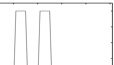
Figure 1: Two rail phantom for 1D deblurring example.

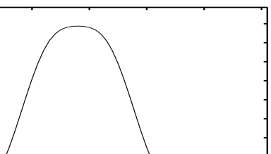
Figure 2: Blurred two level phantom. Blurring kernel is Gaussian with standard width approximately equal to rail separation distance in phantom. An additive randoms noise of 0.3 was added.

For illustration we performed numerical optimization for a simple one dimensional deblurring example under the Poisson noise model of the previous section. This example easily generalizes to more general 2 and 3 dimensional Poisson deblurring, tomographic reconstruction, and other imaging applications. The true source $\theta$ is a two rail phantom shown in Figure 1. The blurring kernel is a Gaussian function yielding the blurred phantom shown in Figure 2. We implemented both EM and KPP with Trust Region update strategy for deblurring Fig. 2 when the set of ideal blurred data $Y_{i}=\sum_{j=1}^{N}P_{ij}\theta_{j}$ is available without Poisson noise. In this simple noiseless case the ML solution is equal to the true source $\theta$ which is everywhere positive. Treatment of this noiseless case allows us to investigate the behavior of the algorithms in the asymptotic high count rate regime. More extensive simulations with Poisson noise will be presented elsewhere.

The numerical results shown in Fig. 3 indicate that the Trust Region implementation of the KPP algorithm enjoys significantly faster convergence towards the optimum than does EM. For these simulations the Trust Region technique was implemented in the standard manner where the trust region size sequence $\delta_{k}$ in Algorithm 1 is determined implicitly by the $\beta_{k}$ update rule: $\beta_{k+1}=1.6\beta_{k}$ ($\delta_{k}$ is decreased) and otherwise $\beta_{k+1}=0.5\beta_{k}$ ($\delta_{k}$ is increased). The results shown in Fig. 4 validate the theoretical superlinear convergence of the Trust Region iterates as contrasted with the linear convergence rate of the EM iterates. Figure 5 shows the reconstructed profile and demonstrates that the Trust Region updated KPP technique achieves better reconstruction of the original phantom for a fixed number of iterations. Finally, Figure 6 shows the iterates for the reconstructed phantom, plotted as a function of iteration on the horizontal axis and as a function of grey level on the vertical axis. Observe that the KPP achieves more rapid separation of the two components in the phantom than does standard EM.

7 Conclusions

The main contributions of this paper are the following. First, we introduced a general class of iterative methods for ML estimation based on Kullback-Liebler relaxation of the proximal point strategy. Next, we proved that the EM algorithm belongs to the proposed class, thus providing a new and useful interpretation of the EM approach for ML estimation. Finally, we showed that Kullback proximal point methods enjoy global convergence and even superlinear convergence for sequences of positive relaxation parameters that converge to zero. Implementation issues were also discussed and we proposed second order schemes for the case where the maximization step is hard to obtain in closed form. We addressed Trust Region methodologies for the updating of the relaxation parameters. Computational experiments indicated that the approximate second order KPP is stable and verifies the superlinear convergence property as was predicted by our analysis.

Stéphane Chrétien - Biosketch

Stéphane Chrétien was born in Rennes, France in 1969. He received the B.S. and the Ph.D in Electrical Engineering from Université Paris Sud-Orsay in 1992 and 1996 respectively. He then hold a postdoctoral position at the EECS department of the University of Michigan, Ann Arbor and a research position at INRIA Rhône-Alpes, France. He is now with the Service de Mathématiques de la Gestion at the Université Libre de Bruxelles, Belgium. His current research interests are in statistical estimation and computational optimization with applications to image reconstruction and urban traffic modelling and control.

Alfred Hero - Biosketch

Alfred O. Hero III, was born in Boston, MA. in 1955. He received the B.S. in Electrical Engineering (summa cum laude) from Boston University (1980) and the Ph.D from Princeton University (1984), both in Electrical Engineering. While at Princeton he held the G.V.N. Lothrop Fellowship in Engineering. Since 1984 he has been with the Dept. of Electrical Engineering and Computer Science at the University of Michigan, Ann Arbor, where he is currently Professor and Director of the Communications and Signal Processing Laboratory. He has held positions of Visiting Scientist at M.I.T. Lincoln Laboratory (1987 - 1989), Visiting Professor at Ecole Nationale des Techniques Avancees (ENSTA), Ecole Superieure d’Electricite, Paris (1990), Ecole Normale Supérieure de Lyon (1999), and Ecole Nationale Supérieure des Télécommunications, Paris (1999), William Clay Ford Fellow at Ford Motor Company (1993). His current research interests are in the area of estimation and detection, statistical communications, signal processing, and image processing. Alfred Hero is a Fellow of the Institute of Electrical and Electronics Engineers (IEEE), a member of Tau Beta Pi, the American Statistical Association (ASA), and Commission C of the International Union of Radio Science (URSI). He received the 1998 IEEE Signal Processing Society Meritorious Service Award, the 1998 IEEE Signal Processing Society Best Paper Award, and the IEEE Third Millenium Medal.

He has served as Associate Editor for the IEEE Transactions on Information Theory. He was also Chairman of the Statistical Signal and Array Processing (SSAP) Technical Committee of the IEEE Signal Processing Society. He served as treasurer of the Conference Board of the IEEE Signal Processing Society. He was Chairman for Publicity for the 1986 IEEE International Symposium on Information Theory (Ann Arbor, MI). He was General Chairman for the 1995 IEEE International Conference on Acoustics, Speech, and Signal Processing (Detroit, MI). He was co-chair for the 1999 IEEE Information Theory Workshop on Detection, Estimation, Classification and Filtering (Santa Fe, NM) and the 1999 IEEE Workshop on Higher Order Statistics (Caesaria, Israel). He is currently a member of the Signal Processing Theory and Methods (SPTM) Technical Committee and Vice President (Finances) of the IEEE Signal Processing Society. He is also currently Chair of Commission C (Signals and Systems) of the US delegation of the International Union of Radio Science (URSI).

Figure 3: Snapshot of log–Likelihood vs iteration for plain EM and KPP EM algorithm. Plain EM initially produces greater increases in likelihood function but is overtaken by KPP EM at 7 iterations and thereafter.

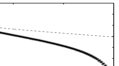
Figure 4: The sequence $\log\|\theta_{k}-\theta^{*}\|$ vs iteration for plain EM and KPP EM algorithms. Here $\theta^{*}$ is limiting value for each of the algorithms. Note the superlinear convergence of KPP.

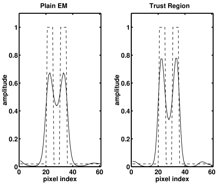
Figure 5: Reconstructed images after 150 iterations of plain EM and KPP EM algorithms.

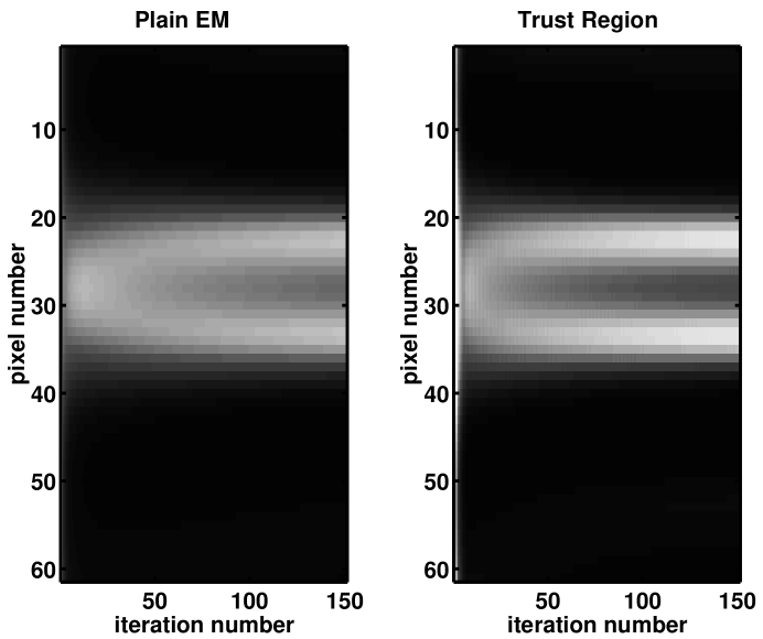
Figure 6: Evolution of the reconstructed source vs iteration for plain EM and KPP EM.

References

- [1] A. A. Goldstein and I. B. Russak, “How good are the proximal point algorithms?,” Numer. Funct. Anal. and Optimiz., vol. 9, no. 7-8, pp. 709–724, 1987.
- [2] H. H. Bauschke and J. M. Borwein, “On projection algorithms for solving convex feasibility problems,” SIAM Review, vol. 38, no. 3, pp. 367–426, 1996.
- [3] J. F. Bonnans, J.-C. Gilbert, C. Lemaréchal, and C. Sagastizabal, Optimization numérique. Aspects théoriques et pratiques, volume 27, Springer Verlag, 1997. Series : Mathématiques et Applications.
- [4] C. Bouman and K. Sauer, “Fast numerical methods for emission and transmission tomographic reconstruction,” in Proc. Conf. on Inform. Sciences and Systems, Johns Hopkins, 1993.
- [5] Y. Censor and S. A. Zenios, “Proximal minimization algorithm with D-functions,” Journ. Optim. Theory and Appl., vol. 73, no. 3, pp. 451–464, June 1992.
- [6] S. Chrétien and A. Hero, “Generalized proximal point algorithms,” SIAM Journ. on Optimization, Submitted Sept., 1998.
- [7] T. Cover and J. Thomas, Elements of Information Theory, Wiley, New York, 1987.
- [8] A. P. Dempster, N. M. Laird, and D. B. Rubin, “Maximum likelihood from incomplete data via the EM algorithm,” J. Royal Statistical Society, Ser. B, vol. 39, no. 1, pp. 1–38, 1977.
- [9] P. Eggermont, “Multiplicative iterative algorithms for convex programming.,” Linear Algebra Appl., vol. 130, pp. 25–42, 1990.
- [10] J. Ekstein, “Nonlinear proximal point algorithms using Bregman functions, with applications to convex programming,” Math. Oper. Res., vol. 18, no. 1, pp. 203–226, February 1993.
- [11] R. Fletcher, “A new variational result for quasi-Newton formulae.,” SIAM J. Optim., vol. 1, no. 1, pp. 18–21, 1991.
- [12] J. C. Gilbert and C. Lemarechal, “Some numerical experiments with variable-storage quasi-Newton algorithms.,” Math. Program., Ser. B, vol. 45, no. 3, pp. 407–435, 1989.
- [13] P. J. Green, “On the use of the EM algorithm for penalized likelihood estimation,” J. Royal Statistical Society, Ser. B, vol. 52, no. 2, pp. 443–452, 1990.
- [14] D. Helmbold, R. Schapire, S. Y., and W. M., “A comparison of new and old algorithms for a mixture estimation problem,” Journal of Machine Learning, vol. 27, no. 1, pp. 97–119, 1997.
- [15] A. O. Hero and J. A. Fessler, “Convergence in norm for alternating expectation-maximization (EM) type algorithms,” Statistica Sinica, vol. 5, no. 1, pp. 41–54, 1995.
- [16] J. B. Hiriart-Hurruty and C. Lemaréchal, Convex analysis and minimization algorithms I-II, Springer-Verlag, Bonn, 1993.
- [17] H. Hudson and R. Larkin, “Accelerated image reconstruction using ordered subsets of projection data,” IEEE Transactions on Medical Imaging, vol. 13, no. 12, pp. 601–609, 1994.
- [18] I. A. Ibragimov and R. Z. Has’minskii, Statistical estimation: Asymptotic theory, Springer-Verlag, New York, 1981.
- [19] M. Jamshidian and R. I. Jennrich, “Conjugate gradient acceleration of the EM algorithm,” J. Am. Statist. Assoc., vol. 88, no. 421, pp. 221–228, 1993.
- [20] L. Kaufman, “Implementing and accelerating the EM algorithm for positron emission tomography,” IEEE Trans. on Medical Imaging, vol. MI-6, no. 1, pp. 37–51, 1987.
- [21] J. Kivinen and M. K. Warmuth, “Additive versus exponentiated gradient updates for linear prediction,” Information and Computation, vol. 132, pp. 1–64, January 1997.
- [22] K. Lange, “A quasi-newtonian acceleration of the EM algorithm,” Statistica Sinica, vol. 5, no. 1, pp. 1–18, 1995.
- [23] K. Lange and R. Carson, “EM reconstruction algorithms for emission and transmission tomography,” Journal of Computer Assisted Tomography, vol. 8, no. 2, pp. 306–316, April 1984.
- [24] D. Lansky and G. Casella, “Improving the EM algorithm,” in Computing and Statistics: Proc. Symp. on the Interface, C. Page and R. LePage, editors, pp. 420–424, Springer-Verlag, 1990.
- [25] M. Lavielle, “Stochastic algorithm for parametric and non-parametric estimation in the case of incomplete data,” Signal Processing, vol. 42, no. 1, pp. 3–17, 1995.
- [26] R. Lewitt and G. Muehllehner, “Accelerated iterative reconstruction for positron emission tomography,” IEEE Trans. on Medical Imaging, vol. MI-5, no. 1, pp. 16–22, 1986.
- [27] D. C. Liu and J. Nocedal, “On the limited memory BFGS method for large scale optimization.,” Math. Program., Ser. B, vol. 45, no. 3, pp. 503–528, 1989.
- [28] T. A. Louis, “Finding the observed information matrix when using the EM algorithm,” J. Royal Statistical Society, Ser. B, vol. 44, no. 2, pp. 226–233, 1982.
- [29] B. Martinet, “Régularisation d’inéquation variationnelles par approximations successives,” Revue Francaise d’Informatique et de Recherche Operationnelle, vol. 3, pp. 154–179, 1970.
- [30] I. Meilijson, “A fast improvement to the EM algorithm on its own terms,” J. Royal Statistical Society, Ser. B, vol. 51, no. 1, pp. 127–138, 1989.
- [31] G. J. Minty, “Monotone (nonlinear) operators in Hilbert space,” Duke Math. Journal, vol. 29, pp. 341–346, 1962.
- [32] J. J. Moré, “Recent developments in algorithms and software for trust region methods,” in Mathematical programming: the state of the art, pp. 258–287, Springer-Verlag, Bonn, 1983.
- [33] J. J. Moreau, “Proximité et dualité dans un espace Hilbertien,” Bull. Soc. Math. France, vol. 93, pp. 273–299, 1965.
- [34] J. Nocedal and S. J. Wright, Numerical optimization, Springer Series in Operations Research, Springer Verlag, Berlin, 1999.
- [35] J. Nocedal, “Updating quasi-Newton matrices with limited storage.,” Math. Comput., vol. 35, pp. 773–782, 1980.
- [36] J. M. Ollinger and D. L. Snyder, “A preliminary evaluation of the use of the EM algorithm for estimating parameters in dynamic tracer studies,” IEEE Trans. Nuclear Science, vol. NS-32, pp. 3575–3583, Feb. 1985.
- [37] J. M. Ortega and W. C. Rheinboldt, Iterative Solution of Nonlinear Equations in Several Variables, Academic Press, New York, 1970.
- [38] R. T. Rockafellar, “Monotone operators and the proximal point algorithm,” SIAM Journal on Control and Optimization, vol. 14, pp. 877–898, 1976.
- [39] L. A. Shepp and Y. Vardi, “Maximum likelihood reconstruction for emission tomography,” IEEE Trans. on Medical Imaging, vol. MI-1, No. 2, pp. 113–122, Oct. 1982.
- [40] M. Teboulle, “Entropic proximal mappings with application to nonlinear programming,” Mathematics of Operations Research, vol. 17, pp. 670–690, 1992.
- [41] M. Warmuth and K. Azoury, “Relative loss bounds for on-line density estimation with the exponential family of distributions,” Proc. of Uncertainty in Artif. Intel., 1999.
- [42] C. F. J. Wu, “On the convergence properties of the EM algorithm,” Annals of Statistics, vol. 11, pp. 95–103, 1983.