COULD COSMIC RAYS AFFECT INSTABILITIES IN THE TRANSITION LAYER OF NONRELATIVISTIC COLLISIONLESS SHOCKS?

Abstract

There is an observational correlation between astrophysical shocks and non-thermal particle distributions extending to high energies. As a first step toward investigating the possible feedback of these particles on the shock at the microscopic level, we perform particle-in-cell (PIC) simulations of a simplified environment consisting of uniform, interpenetrating plasmas, both with and without an additional population of cosmic rays. We vary the relative density of the counterstreaming plasmas, the strength of a homogeneous parallel magnetic field, and the energy density in cosmic rays. We compare the early development of the unstable spectrum for selected configurations without cosmic rays to the growth rates predicted from linear theory, for assurance that the system is well represented by the PIC technique. Within the parameter space explored, we do not detect an unambiguous signature of any cosmic-ray-induced effects on the microscopic instabilities that govern the formation of a shock. We demonstrate that an overly coarse distribution of energetic particles can artificially alter the statistical noise that produces the perturbative seeds of instabilities, and that such effects can be mitigated by increasing the density of computational particles.

1 Introduction

Shocks form in a wide variety of astrophysical environments, from planetary bow shocks in the heliosphere to colliding clusters of galaxies. The presence of nonthermal particle populations in some of these environments is inferred from radio, X-ray, and $\gamma$-ray observations (Reynolds, 2008), and a number of theoretical mechanisms link strong shocks (such as those found in young supernova remnants) to particle acceleration processes (e.g., Drury, 1983; Webb et al., 1983). An understanding of the nonlinear coupling between the shock, the energetic particles, and the spectrum of any excited waves is essential to the proper interpretation of the observational signatures of shocked systems as well as to a correct understanding of the origin of cosmic rays.

In most cases the density of the shocked medium is sufficiently low for collisions between particles to be infrequent; such collisionless shocks are mediated through collective electromagnetic effects. The thickness of the shock transition region and the nature of the microphysics occurring therein may play a key role in the injection efficiency of thermal particles into the acceleration processes thought to accelerate cosmic rays to high energy (Bell, 1978a, b; Scholer et al., 2002). In addition, efficient particle acceleration associated with some shock environments raises the question of the extent to which a significant cosmic-ray contribution to the local energy density can influence the structure of the shock front itself. This may be of particular importance in starburst galaxies, where massive stars and frequent supernovae increase the availability of sites for particle acceleration. The emission of TeV $\gamma$-rays from some nearby starburst galaxies suggests an abundance of cosmic rays that significantly exceeds the values observed locally (Acciari et al., 2009).

A number of mechanisms exist whereby cosmic rays may play a role in shaping the shock and its environment. A significant cosmic-ray contribution to the pressure upstream of a shock is understood to result in substantial modification to the shock environment (Eichler, 1984); this effect is expected to produce an effective shock compression ratio that is perceived as being larger by cosmic rays of higher energy, possibly hardening the local cosmic-ray source spectrum (Malkov and Drury, 2001). Under some conditions, the current carried by cosmic-ray ions diffusing ahead of the shock may excite instabilities in the upstream interstellar medium that lead to large-amplitude magnetic turbulence (Bell, 2004; Lemoine and Pelletier, 2011; Rabinak et al., 2011; Nakar et al., 2011) or other substantial alterations to the upstream environment, such as the heating of thermal electrons (e.g., Rakowski et al., 2008). However, these effects occur on spatial scales much larger than the thickness of the subshock and may operate quite independently of the processes occurring therein.

In this paper, we turn our attention to those processes within the subshock. In order to quantify or constrain the effect of a “spectator” population of cosmic rays (that is, any cosmic rays present that have already been accelerated, locally or elsewhere) on the formation and evolution of nonrelativistic collisionless subshocks, we design simulations to explore the initial linear and subsequent nonlinear growth of instabilities that contribute to shaping the shock transition region. We restrict our focus to the interpenetration layer, in which two counterstreaming plasma shells overlap in space. This is fertile ground for the growth of well-known and well-studied instabilities (Silva et al., 2003; Frederiksen et al., 2004; Bret, 2009), and the two-plasma system will respond accordingly. We then repeat our simulations with an added cosmic-ray component, a plasma consisting of highly relativistic particles, so we may compare the systems at both the early and late stages of their evolution and identify whether the presence of the cosmic rays has any effect.

The scale of the instabilities dictates the computational approach to modeling them. Hydrodynamical models of shocks are incapable of accurately resolving length scales much smaller than a particle mean free path and must therefore approximate subshocks as discontinuities, which is inadequate for our purposes. A self-consistent kinetic approach is necessary for a more complete exploration of the relevant small-scale physical processes, but simulating the entire subshock thickness is prohibitively costly. We elect a simulation that represents only a homogeneous portion of the subshock interior, and therefore we cannot account for a number of instabilities that arise from spatial gradients or particle reflection. Here we use particle-in-cell (PIC) simulations in two spatial dimensions to model the interaction of counterstreaming plasma flows in the presence of a third, hot plasma of energetic particles. The PIC technique is a (particle-based) kinetic approach to modeling the self-consistent evolution of an arbitrary distribution of charged particles and electromagnetic fields and thus is well suited to the nonlinear development of unstable plasma systems. In order to isolate the subshock instabilities from larger-scale spatial effects such as those arising from systematic charge separation, all distribution functions are initially homogeneous with respect to position. We consider the simplified case in which two electron–ion plasmas, not necessarily of equal density, move nonrelativistically through each other. This movement may also be parallel to a uniform magnetic field. We first observe the evolution of the drift velocities, field amplitudes, particle distributions, and wave spectra in the case when cosmic rays are negligible. We then include cosmic rays whose energy density is an order of magnitude below the kinetic energy in the bulk flow of the plasmas. We also explore the case of an artificially high energy density in cosmic rays, exceeding the value of equipartition with the bulk flows, to gain insight into effects that may be too small to arise in the case intended to represent a more realistic environment but that may nevertheless appear in regions where energetic particles are unusually abundant. However, our results suggest that even a high abundance of cosmic rays is not sufficient on its own to produce a significant deviation from the usual evolution of the instabilities shaping a shock.

2 Objectives and approach

To constrain the extent to which cosmic rays might influence the physics of the shock transition layer, we perform a series of simulations. Using the benchmarks of system behavior outlined in Section 2.3, we characterize the response of the counterstreaming-plasma system to the cascade of instabilities arising from interactions among the various plasma components in the absence of cosmic rays. We then repeat the simulations with cosmic rays present, so as to facilitate the side-by-side comparison of the various benchmarks. The parameter choices for the systems that we explore in this manner are described in detail in Section 2.1, and our simulation model and its implementation are described in Section 2.2. Then, a test of selected parameter configurations against the predictions from analytical studies of related systems is described in Section 3. Following a brief discussion, we conclude in Section 5.

2.1 Parameter-space configurations

The physical system under consideration is modeled as one homogeneous electron–ion plasma moving relative to another. These plasmas may in general have different densities. In addition, a uniform magnetic field may be aligned with the flow direction. Finally, a population of cosmic rays may be present, at rest in bulk in the center-of-momentum frame of the two plasmas. This is the reference frame chosen for the simulation, so the two plasmas flow in opposite directions; we adopt the nomenclature of “stream” and “counterstream” to distinguish between them. By our convention, the stream’s velocity is in the $-x$-direction, antiparallel to the guiding magnetic field when one is present.

Our primary simulations are sensitive to variations in three parameters: the density ratio between the stream and the counterstream, the strength of the guiding magnetic field, and the energy density in the cosmic rays.

The inter-plasma density ratio $w\equiv n_{s}/n_{\rm cs}$ takes three values and their respective designations: the “symmetric” case $w=1$, the “intermediate” case $w=0.3$, and the “dilute” case $w=0.1$. The velocity of the stream is fixed at ${\bf v_{s}}=-0.2c{\bf\hat{x}}$, while the velocity of the counterstream obeys the relation $n_{\rm cs}{\bf v_{cs}}+n_{s}{\bf v_{s}}=0$; in the dilute-stream case, the relative flow speed is therefore $0.22c$. Likewise, the density of the counterstream is fixed, so the stream density alone varies; the total electron density $n_{e}$ and thus the electron plasma frequency $\omega_{\rm pe}=\sqrt{e^{2}n_{e}/\epsilon_{0}m_{e}}$ (where $\epsilon_{0}$ is the vacuum permittivity, and $n_{e}=n_{s}+n_{\rm cs}$ is the cumulative electron density) is largest in the symmetric case and reduced by a factor $\sqrt{1.1/2}$ in the dilute case.

The magnetic field $B_{0,x}$ may be absent, or present at either of two amplitudes given by the ratio of the electron cyclotron frequency $\Omega_{e}=eB_{0,x}/m_{e}$ to the electron plasma frequency, $b\equiv\Omega_{e}/\omega_{\rm pe}$. The “absent” magnetic field refers to $b=B_{0,x}=0$. The values designated “weak” and “strong” correspond to $b=0.01$ and $b=0.1$, respectively; in a plasma of electron density of, e.g., $n_{e}\sim 1$ cm^-3, a magnetic field of $\sim 300$ $\mu$G is necessary for $b=0.1$. Since the speed of Alfvén hydromagnetic waves $v_{A}\equiv b\,c/\sqrt{1+m_{i}/m_{e}}$ is at most $0.014c$ for our choice of $m_{i}/m_{e}=50$, all of the plasma collisions we consider have Alfvénic Mach numbers significantly larger than unity (up to $\infty$ in the case when $b=0$). Note that because the electron plasma frequency is not independent of the density ratio $w$ in our simulations, neither is the absolute magnetic-field amplitude corresponding to a particular value of $b$.

All simulations include cosmic-ray particles consisting of electrons and ions, initialized according to an isotropic distribution function and a single speed (Lorentz factor $\gamma_{\rm CR}=50$) whose statistical weight $w_{\rm CR}\equiv n_{\rm CR}/n_{s}$ is adjusted to three levels: “negligible” when $w_{\rm CR}\gamma_{\rm CR}=10^{-8}$, “present” when $w_{\rm CR}\gamma_{\rm CR}=10^{-3}$, and “abundant” when $w_{\rm CR}\gamma_{\rm CR}=10$. Since $w_{\rm CR}$ is defined in terms of the stream density $n_{s}$, the absolute energy density in cosmic rays also varies with the density ratio $w$, being 10 times larger in the symmetric case than the dilute case for each value of $w_{\rm CR}$. Neglecting the contribution of electrons, the bulk kinetic energy in the stream plus counterstream is of order $n_{\rm cs}m_{i}v_{s}^{2}w(1+w)/2$, while the cosmic-ray energy density is of order $n_{\rm CR}\gamma_{\rm CR}m_{i}c^{2}=25w_{\rm CR}\gamma_{\rm CR}wn_{\rm cs}m_{i}v_{s}^{2}$, where we have used the relation $v_{s}/c=0.2$. Thus, the ratio of cosmic-ray energy density to bulk kinetic energy density is $50w_{\rm CR}\gamma_{\rm CR}/(1+w)$: considerably larger than unity for the “abundant” case and a few percent in the “present” case.

2.2 Simulation setup

Our simulations employ a modified version of the relativistic electromagnetic PIC code TRISTAN (Buneman, 1993), updated for parallel use with MPI, operating in two spatial dimensions, with three-component velocity and field vectors (2D3V), with periodic boundary conditions. The charge-conserving current deposition routine of Umeda et al. (2003) and the field update algorithm with fourth-order accuracy from Greenwood et al. (2004) are the most prominent additions, as well as digital filtering of electric currents to suppress small-scale noise via an iterative smoothing algorithm.

The primary set of simulations, 27 in total, was conducted on a spatial grid in the $x$–$y$ plane of size $280\lambda_{\rm se}\times 180\lambda_{\rm se}$ (periodic boundary conditions in $x$ and $y$, with elongation in the flow direction $x$), where $\lambda_{\rm se}\equiv c/\omega_{\rm pe}=10\Delta$ is the electron skin depth, set to 10 grid cells of length $\Delta$. The electron plasma frequency $\omega_{\rm pe}$ is determined from the sum of the stream and counterstream electron densities only and thus depends on $w$ but not on $w_{\rm CR}$. Supplementary high-resolution simulations in which $\lambda_{\rm se}=30\Delta$ were performed on a grid of more cells but representing a smaller physical region, $128\lambda_{\rm se}\times 96\lambda_{\rm se}$. The time step $\delta t$ was chosen such that $\omega_{\rm pe}^{-1}\approx 22\delta t$ for the $\lambda_{\rm se}=10\Delta$ simulations, or $\omega_{\rm pe}^{-1}\approx 66\delta t$ for the high-resolution $\lambda_{\rm se}=30\Delta$ simulations.

Six separate particle populations from three plasmas are modeled: the “stream” moving in the $-x$-direction, the “counterstream” moving in the $+x$-direction, and the energetic particles representing cosmic rays. Within each plasma, ions and electrons of charge $\pm e$ and mass ratio $m_{i}/m_{e}=50$ have equal charge density and a common drift velocity so that the entire setup has no net current and no charge imbalance. The artificially low mass ratio expedites the simulations, but may change some modes (Hellinger et al., 2007). Quite a few of these possibly modified modes are not included here, partly because we do not consider the spatial structure of subshocks, partly because they do not fit onto the computational grid, and partly because we do not simulate situations involving an oblique or a perpendicular large-scale magnetic field. In any case, the analytical treatment of instabilities presented in Section 3 accounts for the small mass ratio, and in that sense our approach is consistent, at least for the linear phase.

Each cell in a primary (high-resolution supplementary) simulation is initialized with a total of 90 (120) computational particles: 20 stream ions, 20 counterstream ions, and 5 (20) cosmic-ray ions; and an electron for each ion. The physical density of each plasma is manipulated through the assignment of the appropriate statistical weights, $w$ and $w_{\rm CR}$, to the various particle species.

The stream and counterstream, viewed from their respective rest frames at $v_{s}=-0.2c\hat{x}$ and $v_{\rm cs}=w\times 0.2c\hat{x}$, are described by a Maxwell–Boltzmann distribution in which the electrons’ most probable speed is given by $v_{{\rm th},e}=0.01c$ and the ions are in equilibrium with the electrons. The cosmic rays, whose rest frame is the simulation frame $v_{\rm CR}=0$, are isotropic and each is initialized with Lorentz factor $\gamma_{\rm CR}=50$, regardless of whether it is an ion or an electron. Placing the cosmic-ray population at rest in the center-of-momentum frame minimizes streaming in the collision zone, and therefore reduces known cosmic-ray-driven instabilities (Achterberg, 1983; Bell, 2004; Reville et al., 2006), which can be independently studied (e.g., Niemiec et al., 2008; Luo and Melrose, 2009; Ohira et al., 2009; Stroman et al., 2009; Riquelme and Spitkovsky, 2009; Gargaté et al., 2010). We are interested in whether or not cosmic rays can modify instabilities operating at subshocks, and therefore suppress cosmic-ray streaming instabilities .

2.3 Behavioral benchmarks

To provide a basis for comparison among different cosmic-ray densities $w_{\rm CR}$ for each combination of plasma density ratio $w$ and magnetic-field amplitude $b$, we select the following attributes of the system for study: the drift velocity of each particle population, the instantaneous root-mean-square amplitude of the parallel and perpendicular components of the electric and magnetic field over the entire simulation domain, the effective temperature of each stream or counterstream particle species, and the spectrum of excited wave modes in the magnetic field.

As there is no initial bulk motion in the perpendicular directions, only the parallel component $V_{x}$ of drift velocity is considered. The electric field amplitudes are presented in units of the scaling electric field $E_{\omega}\equiv\omega_{\rm pe}\,c\,m_{e}/e$ (equivalent to the field at which the electric energy density is half the electrons’ rest-mass energy density, $\epsilon_{0}E^{2}/2=N_{e}m_{e}c^{2}/2$); the magnetic field multiplied by $c$ is expressible in the same units.

The particle distributions may not remain strictly Maxwellian throughout the duration of the simulation. As a surrogate for temperature, therefore, the mean random kinetic energy of the electrons and ions of the stream and counterstream is calculated by determining the systematic velocity component within a $10\Delta\times 10\Delta$ region and eliminating this local bulk motion via an appropriate Lorentz transformation; the mean post-transformation Lorentz factor $\gamma^{\prime}$ corresponds only to the random motion.

Finally, we will explore the effect of cosmic rays on the time evolution of the spectral decomposition of the perpendicular (out-of-plane) magnetic field $B_{z}$ into its spatial Fourier components, both parallel (wave number $k_{x}=k_{\parallel}$) and perpendicular to the drift (wave number $k_{y}=k_{\perp}$).

3 Comparison with analytical beam–plasma predictions

As a test that our simulation results were consistent with theory, we applied the methods of Bret (2009) to selected stream–counterstream configurations without cosmic rays. Whether magnetized or not, beam–plasma systems (in which a fast, dilute “beam” plays a role comparable to that of our stream, with the dense “plasma” representing our counterstream) are susceptible to a host of both electrostatic and electromagnetic instabilities. For flow-aligned wave vectors, electrostatic modes such as two-stream or Buneman are likely to grow. In the direction normal to the flow, the filamentation instability (sometimes referred to as “Weibel”) is usually excited as well. Finally, modes with wave vectors oriented obliquely are likewise unstable, so that the unstable spectrum is eventually at least two dimensional.

The full spectrum has been first evaluated solving the exact dispersion equation in the cold approximation, accounting thus for a guiding magnetic field as well as finite-mass ions. It turns out that for the present configuration, ions play a very limited role (in the linear phase) and are not responsible for any unstable modes which would not be excited if they were infinitely massive. Unlike settings exhibiting nonresonant modes, for example (Bell, 2004; Stroman et al., 2009), where a single proton beam is considered without electrons moving at the same speed, we are here dealing with a plasma-shell collision, where protons and electrons are comoving. As a result, the effect of finite-mass ions is simply a first-order correction to the electronic spectrum. The dispersion equation displays the very same branches, and the growth rate is altered by a quantity proportional to $\mathcal{O}(m_{e}/m_{i})$.

The dispersion equation for arbitrarily oriented modes with the flow along the $x$-axis reads (Bret et al., 2010)

$$(\omega^{2}\epsilon_{xx}-k_{y}^{2}c^{2})(\omega^{2}\epsilon_{yy}-k_{x}^{2}c^{2})-(\omega^{2}\epsilon_{xy}-k_{y}k_{x}c^{2})^{2}=0,$$ (1)

where the tensor elements $\epsilon_{\alpha\beta}$ are given by

$$\epsilon_{\alpha\beta}(\mathbf{k},\omega)=\delta_{\alpha\beta}+\sum_{j}\frac{\omega_{pj}^{2}}{\omega^{2}}\int d^{3}p\,\frac{p_{\alpha}}{\gamma(\mathbf{p})}\frac{\partial f_{j}^{0}}{\partial p_{\beta}}+\sum_{j}\frac{\omega_{pj}^{2}}{\omega^{2}}\int d^{3}p\,\frac{p_{\alpha}p_{\beta}}{\gamma(\mathbf{p})^{2}}\frac{\mathbf{k}\cdot\left(\frac{\partial f_{j}^{0}}{\partial\mathbf{p}}\right)}{m_{j}\omega-\mathbf{k}\cdot\mathbf{p}/\gamma(\mathbf{p})},$$ (2)

and the sum runs over the species involved in the system. For each species, the distribution function $f_{j}^{0}$ includes both the stream and the counterstream, and the corresponding plasma frequency $\omega_{pj}$ is calculated using the sum of their densities. The results in the cold-plasma limit are evaluated considering Dirac’s delta distribution functions. Though lengthy, calculations are straightforward. Setting $k_{y}=k_{\perp}=0$ in the equations above allows to derive the dispersion equation for flow-aligned modes such as the two-stream ones. Setting $k_{x}=k_{\parallel}=0$ gives the dispersion equation for the filamentation modes. We present analytical results for the symmetric and the diluted beam cases. While such expressions can be derived considering either $w=1$ or $w\ll 1$, expressions valid for any density ratio $w$ are much more involved (when they exist). This explains why the results below for $w=1$ cannot be derived from those with $w\ll 1$.

For flow-aligned wave vectors, the most unstable wave vector $k_{\parallel,m}$ and maximum growth rate $\gamma_{m}$ read (with evaluation corresponding to the configuration displayed in Figure 1)

$$k_{\parallel,m}\lambda_{\rm se}\frac{\Delta v}{c} = \frac{\sqrt{3}\sqrt{1+m_{e}/m_{i}}}{\sqrt{2}\Gamma_{s}^{3/2}}=1.19,$$

$$\frac{\gamma_{m}}{\omega_{\rm pe}} = \frac{\sqrt{1+m_{e}/m_{i}}}{\sqrt{2}\Gamma_{s}^{3/2}}=0.68,~{}~{}\mathrm{symmetric~{}case},$$ (3)

and

$$k_{\parallel,m}\lambda_{\rm se}\frac{\Delta v}{c} = \sqrt{1+w}=1.04,~{}~{}w\ll 1$$

$$\frac{\gamma_{m}}{\omega_{\rm pe}} = \frac{\sqrt{3(1+w)}}{2^{4/3}}\frac{w^{1/3}(1+m_{e}/m_{i})^{1/3}}{\Gamma_{s}}=0.31,~{}~{}\mathrm{dilute~{}case},$$ (4)

where $\Gamma_{s}=\left(1-{v_{s}}^{2}/c^{2}\right)^{-1/2}$ is the bulk Lorentz factor of the stream, which moves in the simulation frame with speed $v_{s}=0.417c/(1+w)$. As seen in Figure 1, panels (a) and (f), oblique modes dominate for the mildly relativistic conditions of the simulation. The full-spectrum maximum growth rate is thus slightly larger than the numerical values calculated above for modes propagating along the flow.

For wave vectors normal to the flow, the growth rate reaches its maximum for $k_{\perp}=\infty$, with

$$\frac{\gamma_{m}}{\omega_{\rm pe}}=2\frac{v_{s}}{c}\sqrt{\frac{1+m_{e}/m_{i}}{\Gamma_{s}}}=0.41,~{}~{}\mathrm{symmetric~{}case},$$ (5)

and

$$\frac{\gamma_{m}}{\omega_{\rm pe}}=\frac{v_{s}}{c}\sqrt{\frac{w(1+w)(1+m_{e}/m_{i})}{\Gamma_{s}}}=0.12,~{}~{}\mathrm{dilute~{}case}.$$ (6)

These filamentation data have been calculated neglecting the magnetic field, which is small ($\Omega_{e}=0.01\omega_{\rm pe}$) in the present setup. Electrostatic unstable modes propagating along the flow are rigorously insensitive to the flow-aligned magnetic field. As long as $m_{e}/m_{i}\ll 1$, the two-dimensional linear spectra computed with or without finite-mass protons are indistinguishable. The hot spectra, accounting for the $v_{{\rm th},e}=0.01c$ thermal spread for the electrons, have then been calculated considering infinitely heavy protons and using the fluid approximation described in Bret and Deutsch (2006).

The predicted growth rates for the two-dimensional $k_{\parallel}$,$k_{\perp}$ wave-vector space are plotted in Figure 1, panels (b) and (g) for the dilute and symmetric streams, respectively, when the stream velocity is $0.417c$ (corresponding to a bulk Lorentz factor $\Gamma_{\rm rel}=1.1$) relative to the counterstream. To better accommodate the parameters available for the calculations, it was necessary to make slight adjustments to the simulations we performed for comparison, leading to an increase in both the ion mass and, in the dilute case, the relative drift speed between the plasmas. The calculations also make predictions for modes at very large wavelengths in both spatial dimensions. We therefore repeated the early stage of our simulation with the comparison parameters $m_{i}/m_{e}=100$ and $\Gamma_{\rm rel}=1.1$, on an enlarged grid of $3840\Delta\times 3840\Delta$, and $\lambda_{\rm se}=30\Delta$.

To make a comparison with the analytical predictions, we extract the two-dimensional ${\bf k}$ spectrum at times separated by only a short interval intended to capture the earliest linear growth of the instabilities, and compute the average growth rate, which is plotted in Figure 1 panels (c)–(e) and (h)–(j) for the dilute and symmetric cases, respectively. The agreement is satisfactory, both qualitatively and quantitatively, and the dominant modes are correctly rendered. As expected, the cold theoretical spectrum saturates at high $k_{\perp}$ while the hot version displays a local extremum for an oblique wave vector, as the kinetic pressure prevents the pinching of high-$k_{\perp}$ small filaments (Silva et al., 2002).

Moreover, for high $k_{\perp}$, the PIC spectrum describes wavelengths only a few cells long, small enough to be affected by the smoothing algorithm. This explains why these modes’ growth is slower than expected. An electron skin depth of several hundred cells would almost certainly provide sufficient separation from the filtering length for the plots to agree better with the theoretical ones in this region, but such a simulation could not be large enough, or run long enough, to observe the later evolution without prohibitive computational expense.

Modes with $k_{\perp}=0$ are purely electrostatic, and produce no magnetic field. This is why their growth rate is much better rendered when measuring the $E$ spectrum rather than the $B$ spectrum. Conversely, modes with $k_{\parallel}=0$ are mostly electromagnetic with a very small phase velocity, which explains why their growth is only evident in the $B$ spectrum.

4 Results

The qualitative behavior of the counterstreaming-plasma system in the absence of cosmic rays exhibits a dependence on the density ratio $w$ particularly in the earliest stages of evolution, and at later times the impact of the magnetic field $b$ becomes prominent. Although the details differ from one simulation to the next, the general behavior is similar to that seen in the three-dimensional simulations of Frederiksen et al. (2004), in which the collision of electron–ion plasmas is characterized by the formation of current channels first in the electrons, and later in the ions, which proceed to merge and grow. In our experiments, this growth of the channels and associated structure in the magnetic field eventually reaches a size comparable to the simulation domain, at which point the imposed periodic boundary conditions prevent further enlargement. However, the time necessary for this to occur—hundreds or thousands of $\omega_{\rm pe}^{-1}$—may exceed the residence time of a given particle in the subshock.

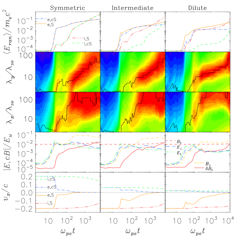
Figure 3: Selected results from the “negligible-weak” family of simulations. The initial magnetic field is set such that the electron cyclotron frequency is $\Omega_{e}\equiv e\,B/m_{e}=0.01\omega_{\rm pe}$. See the caption to Figure 2 for a detailed description of each plot.

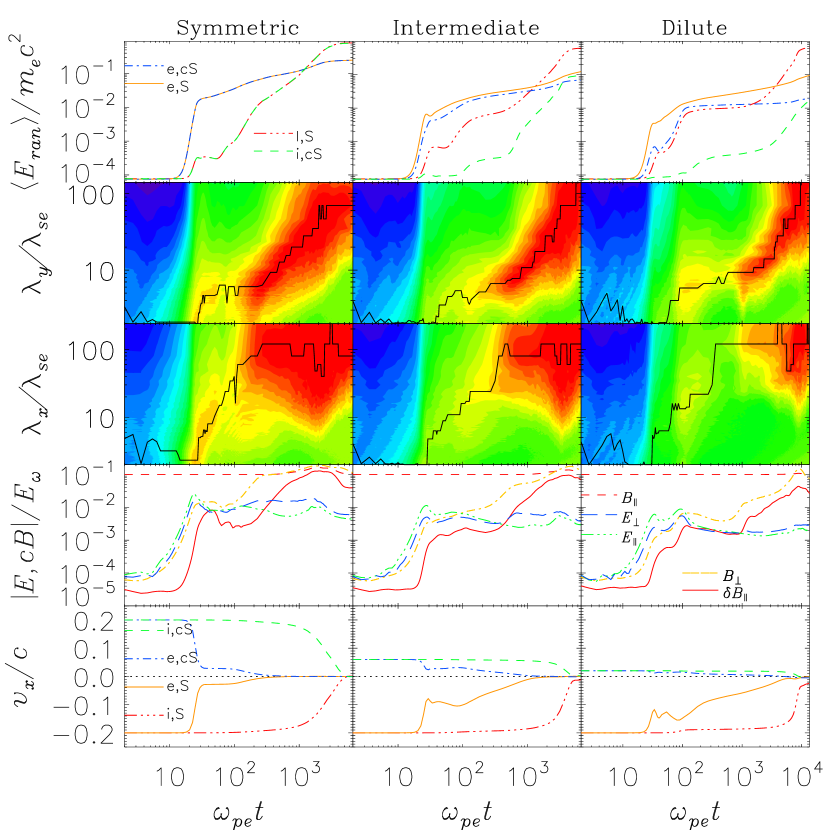
Figure 4: Selected results from the “negligible-strong” family of simulations. The initial magnetic field is set such that the electron cyclotron frequency is $\Omega_{e}=0.1\omega_{\rm pe}$. See the caption to Figure 2 for a detailed description of each plot.

The benchmark behavior for our simulations of negligible-cosmic-ray energy density is plotted in Figure 2 (magnetic field absent), Figure 3 (weak magnetic field), and Figure 4 (strong magnetic field); the three columns of each plot correspond to the symmetric, intermediate, and dilute density ratios $w$. The role of the density ratio is prominent in the action of the two-stream instability on the drift velocity of the counterstreaming electron populations (Medvedev and Loeb, 1999). For all considered values of magnetic field $b$, there is an abrupt deceleration of the electrons, both the stream and counterstream, when $20<\omega_{\rm pe}t<30$. In the $w=1$ symmetric case, this initial deceleration strips the electrons of nearly 90% of their relative drift, but in the dilute case, less than half the drift is removed. The electric and magnetic fields are amplified substantially at this point, but the reduced electron drift suppresses further immediate amplification. The ions are slower to respond, and their evolution differs qualitatively from that of the electrons: they form spatially alternating long-lived channels of current: as in lanes of vehicular traffic, ions moving one direction become spatially segregated from those moving the opposite direction, and this greatly lengthens the time for the ion drift velocities to converge, though considerable heating of the ions takes place prior to any significant systematic deceleration.

The convergence of ion drift velocities reveals the primary effect of the magnetic field: the ion speeds remain well separated throughout the simulation lifetime in the absent or weak magnetic-field cases, but the strong magnetic field brings them together within roughly $10^{4}\omega_{\rm pe}^{-1}$ for all density ratios. It may be that at least in this two-dimensional simulation, the transverse motion necessary for separating the ions into current channels is slightly inhibited by the guiding magnetic field, increasing the extent to which the counterstreaming ion populations are forced to interact. However, it is worth noting once more that the late-term behavior of the simulations is suspect on account of the structure size becoming comparable to the domain boundaries, an artificial upper limit.

4.1 Behavior including cosmic rays

For the configurations we considered, the presence of cosmic rays does not appear to result in any significant deviations from the behavior observed in their absence. When their energy density is given a value intended to represent conditions typical of the Galactic disk, no differences from the negligible-cosmic-ray configuration are observed. When cosmic rays are given an exaggerated abundance, subtle effects do appear in the simulation, but upon inspection they are disregarded for one of two reasons: they can be dismissed as numerical effects arising from the finite number of cosmic-ray particles employed in our simulation, or else they result in minor quantitative changes in the evolution that are of greatest prominence only when the effect of the periodic boundaries is already non-negligible. When the cosmic-ray weight is comparable to that of the plasma particles, their speed (approximately $c$) maximizes the amplitude of current-density fluctuations resulting from the statistically expected local departures from homogeneity.

In order to verify that the observed differences resulted from our choice of representation and not from some underlying physics, we repeated an “abundant” simulation with a tenfold increase in computational particles representing the same physical cosmic-ray density. Figure 5 illustrates via the electromagnetic field amplitudes that the statistical noise levels arising at the earliest times saturate at a level $\sqrt{10}$ lower when cosmic rays are represented by 50 particles per cell instead of 5, bringing both the noise level and the detailed time evolution into better agreement with the “negligible” case. A further significant increase in the computational particle count is too expensive for direct comparison with the simulations in Figure 5. Using a smaller computational grid, a simulation with 500 cosmic-ray particles per cell (leaving the other plasmas at their original 20 per cell) illustrates the continuation of the trend observed with 50 per cell. Nevertheless, the remaining difference in non-noise behavior is already nearly imperceptible at just 50 computational particles per cell. This effect is paralleled in the other aspects of the system’s evolution in which abundant cosmic rays appeared to result in minor differences, such as drift velocities and wave spectra.

5 Discussion and conclusions

Motivated by an interest in possible effects of cosmic rays on the physics governing the development of collisionless astrophysical shocks, we have performed several multidimensional PIC simulations of counterstreaming plasmas with various density ratios and magnetic-field strengths, both with and without a background population of energetic cosmic rays. This initially homogeneous environment is intended to represent the interior of the subshock, or shock transition layer. Before cosmic rays are added to the picture, the system resembles the subject of numerous beam–plasma or interpenetrating-plasma studies, where the initial behavior of the system can be understood in terms of known instabilities. Most prominently, the counterstreaming electron populations are the first to interact, via symmetric or asymmetric two-stream instabilities, as seen in, e.g., Medvedev and Loeb (1999) and Frederiksen et al. (2004). In particular, the three-dimensional simulations of unmagnetized electron–ion plasma collisions by Frederiksen et al. (2004) demonstrate the formation of merging and growing current filaments in first the electrons and subsequently the ions, and the nuanced relationships among the various populations.

One limitation of our approach is the reduced electron–ion mass ratio, $m_{e}/m_{i}=1/50$. Bret and Dieckmann (2010) have explored the effect of the mass ratio on the hierarchy of unstable modes in beam–plasma systems. By stating that a mass ratio different from 1/1836 should not change the nature of the most unstable mode, they were able to articulate a criterion defining the largest acceptable mass ratio. In the present case, the unstable linear spectrum depends very weakly on the mass ratio, when no cosmic rays are introduced. As stated in Section 3, finite-mass ions do not add any extra unstable branches to the dispersion equation. As a result, the Bret–Dieckmann criterion is necessarily fulfilled in our configuration without cosmic rays. Turning now to the simulations including cosmic rays, we found no significant cosmic-ray effects with our current mass ratio within the cosmic-ray population. It is thus likely that a real mass ratio would result in an even weaker effect, leaving our conclusions unchanged.

Even at just 50 times the electron mass, however, the behavior of the ions is markedly different. For the most part, the electrons produce and respond to turbulent small-scale electromagnetic fields that serve to mix their distribution functions; the electrons act in concert as a single population while the ions of the stream are still easily distinguished from the ions of the counterstream on account of the filaments. Only when the filamentary structures have enlarged until relatively few repetitions are contained within the simulation plane do the ions begin to converge, and in some of our simulations that remains speculative on account of their finite duration. While it would be possible to extend the simulations ostensibly to observe the eventual convergence, this would be of limited value without simultaneously increasing the dimensions of the simulation domain to mitigate the effect of the periodic boundary conditions. An appreciable increase in size, however, may require us to abandon the simplicity of our present configuration by taking into account large-scale spatial variations, perhaps involving a clear distinction between upstream and downstream regions and an unstable charge-separation layer resulting from differences in the electrons’ and ions’ evolution.

When we compare the system evolution in the presence of cosmic rays with that in their absence, we find that for the physical configurations studied, cosmic rays do not introduce a statistically significant departure from the unperturbed results described in Section 4. This may be a consequence of the comparatively large mean free path and characteristic timescale for evolution of the cosmic-ray distribution: even with the amplification of electric and magnetic fields within the transition layer, cosmic rays of modest energy apparently do not couple to the dynamics of thermal electrons and ions in any appreciable way. We surmise that at least for unmagnetized or parallel subshocks, the impact of cosmic rays—even when their energy density is unusually large—on the instabilities mediating the subshock transition is negligible.

Cosmic rays may still indirectly affect various properties of the shock, by modifying the upstream environment from its quiescent characteristics (Stroman et al., 2009): a shock will of necessity propagate differently through a turbulent, heated upstream medium—perhaps with a greatly amplified magnetic field—from the comparatively clean case of a uniform, cold interstellar medium in a gently fluctuating Galactic magnetic field. Irrespective of the cosmic-ray abundance, the rapid development of turbulence in the shock transition layer and the associated heating of the electrons in particular may provide an enlarged pool of candidates for injection into the standard diffusive shock acceleration mechanism.

The combinations of parameters we explored did not yield any appreciable effects that could be attributed to the presence of cosmic rays. While we chose parameters intended to be relevant to nonrelativistic astrophysical shocks in environments where the presence of cosmic rays is suspected, it is nevertheless possible that in other, more exotic environments, cosmic rays may yet play some unforeseen role in the subshock microphysics. Future simulations in three dimensions and assigning additional degrees of freedom to the magnetic field and the cosmic-ray population may uncover effects that eluded the present analysis. However, a departure from the quasiparallel-shock configuration will also introduce effects not observed here, such as the development of magnetosonic waves, which can be more sensitive to the values of the mass ratio or other simulation parameters; this in turn may affect the dissipation of excited unstable modes (see, e.g., Hellinger et al., 2007). In any case, the dearth of differences between even the grossly exaggerated cosmic-ray energy density and the system in which it was negligible provides a sense of reassurance that the physics of perhaps a majority of astrophysical shock-forming instabilities can in principle be understood without invoking some direct microscopic interference by a spectator population of cosmic rays.

This research was supported in part by the National Science Foundation both through TeraGrid resources provided by NCSA (Catlett et al., 2007) and under Grant No. PHY05-51164. The work of A.B. is supported by projects ENE2009-09276 of the Spanish Ministerio de Educación y Ciencia and PEII11-0056-1890 of the Consejería de Educación y Ciencia de la Junta de Comunidades de Castilla-La Mancha. The work of J.N. is supported by MNiSW research project N N203 393034, and The Foundation for Polish Science through the HOMING program, which is supported by a grant from Iceland, Liechtenstein, and Norway through the EEA Financial Mechanism. M.P. acknowledges support through grant PO 1508/1-1 of the Deutsche Forschungsgemeinschaft.

Figure 1: Measured or calculated growth rates (in units of electron plasma frequency) of unstable modes with wave vector $k_{\parallel},k_{\perp}$ (scaled by $\lambda_{\rm se}\Delta v/c$) for the dilute (left column) and symmetric (right column) stream configurations, with negligible-cosmic-ray density and the weak ($b=0.01$) magnetic field. Within each column, the uppermost plot (a, f) is the instantaneous growth rate calculated in the zero-temperature limit. The next plot (b, g) includes a finite thermal spread of $v_{{\rm th},e}=0.01c$ in the calculation. The remaining three rows are the average growth rate measured in the early stages of high-resolution PIC simulations, for the growth of perturbations in $E_{x}$ (c, h), $E_{y}$ (d, i), and $B_{z}$ (e, j). The growth-rate measurement is performed by calculating the fractional increase in the instantaneous two-dimensional Fourier power spectrum for the selected field component between times $t_{0}$ and $t_{1}$. For the dilute configuration, $\omega_{\rm pe}t_{0}\approx 6$ and $\omega_{\rm pe}t_{1}\approx 18$; for the symmetric configuration, $\omega_{\rm pe}t_{0}\approx 6$ and $\omega_{\rm pe}t_{1}\approx 12$. By virtue of being an average over a finite interval, the growth rate obtained in this way is not a pure, instantaneous quantity like the top two rows of plots. The changing conditions in the stream and counterstream alter the instantaneous growth rate during the measurement interval, resulting in the minor differences that appear between the upper and lower parts of each column.

Figure 2: Selected results from the “negligible-absent” family of simulations, in which cosmic rays are negligible and an initial homogeneous magnetic field is absent. From left to right, the density ratio of the stream to the counterstream is $w=1$, 0.3, and 0.1, corresponding to the “symmetric,” “intermediate,” and “dilute” cases, respectively. The bottom row shows the drift velocity of the stream electrons (solid line), stream ions (dot-dot-dot-dashed line), counterstream electrons (dot-dashed line), and counterstream ions (dashed line). A dotted line is included at zero velocity, representing the cosmic-ray ions and electrons. The second-to-bottom row displays the root-mean-square amplitudes of the electric and magnetic field parallel and perpendicular to the drift axis, where the magnetic field has been multiplied by $c$ and all components are expressed in units of $E_{\omega}\equiv\omega_{\rm pe}\,c\,m_{e}/e$. The second and third rows from the top illustrate the time evolution of the Fourier spectra of $B_{z}$ both parallel and perpendicular to the drift, with wavelengths measured in units of the electron skin depth $\lambda_{\rm se}$. A solid black line traces the evolution of the dominant values of $\lambda_{x}$ and $\lambda_{y}$. The top row plots the mean random kinetic energy (i.e., thermal energy) per particle, $E_{\rm ran}=\left(\gamma^{\prime}-1\right)\,m\,c^{2}$, where $\gamma^{\prime}$ is the particle Lorentz factor in the local plasma rest frame (measured over a square-shaped region of area $100\Delta^{2}$). The lines in the top row represent the same populations as in the bottom row.

Figure 5: Evolution of the electric and magnetic field components in the configuration $b=0.1$, $w=0.3$, as a function of the cosmic rays’ computational representation. Panel (a) shows the case when cosmic rays are negligible. The “abundant” ($w_{\rm CR}\gamma_{\rm CR}=10$) cosmic-ray distribution is represented by only five computational particles per cell in panel (c). In panel (e), the number of particles has been increased tenfold, and the initial field amplitudes decrease by approximately $\sqrt{10}$, suggesting that statistical fluctuations in the cosmic-ray contribution to the local current density result in a high noise level in the field components. The column on the right reproduces the conditions of the left column on a grid whose dimensions have been reduced by 90% in each direction, allowing a full-length simulation with 500 cosmic-ray particles per cell. Panels (b) and (d) are comparable to panels (a) and (c), respectively, until $\omega_{\rm pe}t\sim 1000$; the difference beyond this is a result of the smaller grid’s periodic boundaries inhibiting the continued spatial growth of structures earlier. In panel (f), the initial noise level is reduced by a factor of $\sqrt{100}$ in all field components, corroborating our earlier supposition that the higher amplitudes are the effect of statistical noise.

References

- Acciari et al. (2009) Acciari, V. A. et al.: 2009, Nature 462, 770
- Achterberg (1983) Achterberg, A.: 1983, A&A 119, 274
- Bell (1978a) Bell, A. R.: 1978a, MNRAS 182, 147
- Bell (1978b) Bell, A. R.: 1978b, MNRAS 182, 443
- Bell (2004) Bell, A. R.: 2004, MNRAS 353, 550
- Bret (2009) Bret, A.: 2009, ApJ 699, 990
- Bret and Deutsch (2006) Bret, A. and Deutsch, C.: 2006, Physics of Plasmas 13(4), 042106
- Bret and Dieckmann (2010) Bret, A. and Dieckmann, M. E.: 2010, Physics of Plasmas 17(3), 032109
- Bret et al. (2010) Bret, A., Gremillet, L., and Dieckmann, M. E.: 2010, Physics of Plasmas 17(12), 120501
- Buneman (1993) Buneman, O.: 1993, Computer Space Plasma Physics: Simulation Techniques and Software, ed. H. Matsumoto & Y. Omura, pp 67–84, Tokyo: Terra
- Catlett et al. (2007) Catlett, C. et al.: 2007, TeraGrid: Analysis of Organization, System Architecture, and Middleware Enabling New Types of Applications, IOS Press
- Drury (1983) Drury, L. O.: 1983, Reports on Progress in Physics 46, 973
- Eichler (1984) Eichler, D.: 1984, ApJ 277, 429
- Frederiksen et al. (2004) Frederiksen, J. T., Hededal, C. B., Haugbølle, T., and Nordlund, Å.: 2004, ApJ 608, L13
- Gargaté et al. (2010) Gargaté, L., Fonseca, R. A., Niemiec, J., Pohl, M., Bingham, R., and Silva, L. O.: 2010, ApJ 711, L127
- Greenwood et al. (2004) Greenwood, A. D., Cartwright, K. L., Luginsland, J. W., and Baca, E. A.: 2004, Journal of Computational Physics 201, 665
- Hellinger et al. (2007) Hellinger, P., Trávníček, P., Lembège, B., and Savoini, P.: 2007, Geophys. Res. Lett. 34, L14109
- Lemoine and Pelletier (2011) Lemoine, M. and Pelletier, G.: 2011, MNRAS 417, 1148
- Luo and Melrose (2009) Luo, Q. and Melrose, D.: 2009, MNRAS 397, 1402
- Malkov and Drury (2001) Malkov, M. A. and Drury, L. O.: 2001, Reports on Progress in Physics 64, 429
- Medvedev and Loeb (1999) Medvedev, M. V. and Loeb, A.: 1999, ApJ 526, 697
- Nakar et al. (2011) Nakar, E., Bret, A., and Milosavljević, M.: 2011, ApJ 738, 93
- Niemiec et al. (2008) Niemiec, J., Pohl, M., Stroman, T., and Nishikawa, K.: 2008, ApJ 684, 1174
- Ohira et al. (2009) Ohira, Y., Reville, B., Kirk, J. G., and Takahara, F.: 2009, ApJ 698, 445
- Rabinak et al. (2011) Rabinak, I., Katz, B., and Waxman, E.: 2011, ApJ 736, 157
- Rakowski et al. (2008) Rakowski, C. E., Laming, J. M., and Ghavamian, P.: 2008, ApJ 684, 348
- Reville et al. (2006) Reville, B., Kirk, J. G., and Duffy, P.: 2006, Plasma Physics and Controlled Fusion 48, 1741
- Reynolds (2008) Reynolds, S. P.: 2008, ARA&A 46, 89
- Riquelme and Spitkovsky (2009) Riquelme, M. A. and Spitkovsky, A.: 2009, ApJ 694, 626
- Scholer et al. (2002) Scholer, M., Kucharek, H., and Kato, C.: 2002, Physics of Plasmas 9, 4293
- Silva et al. (2003) Silva, L. O., Fonseca, R. A., Tonge, J. W., Dawson, J. M., Mori, W. B., and Medvedev, M. V.: 2003, ApJ 596, L121
- Silva et al. (2002) Silva, L. O., Fonseca, R. A., Tonge, J. W., Mori, W. B., and Dawson, J. M.: 2002, Physics of Plasmas 9, 2458
- Stroman et al. (2009) Stroman, T., Pohl, M., and Niemiec, J.: 2009, ApJ 706, 38
- Umeda et al. (2003) Umeda, T., Omura, Y., Tominaga, T., and Matsumoto, H.: 2003, Computer Physics Communications 156, 73
- Webb et al. (1983) Webb, G. M., Axford, W. I., and Terasawa, T.: 1983, ApJ 270, 537