JACOBI-PREDICTOR-CORRECTOR APPROACH FOR THE FRACTIONAL ORDINARY DIFFERENTIAL EQUATIONS

Abstract.

We present a novel numerical method, called Jacobi-predictor-corrector approach, for the numerical solution of fractional ordinary differential equations based on the polynomial interpolation and the Gauss-Lobatto quadrature w.r.t. the Jacobi-weight function $\omega(s)=(1-s)^{\alpha-1}(1+s)^{0}$. This method has the computational cost $O(N)$ and the convergent order $IN$, where $N$ and $IN$ are, respectively, the total computational steps and the number of used interpolating points. The detailed error analysis is performed, and the extensive numerical experiments confirm the theoretical results and show the robustness of this method.

1. Introduction

This paper further discusses the numerical algorithm for the following initial value problem

$$D^{\alpha}_{\ast}x(t)=f\big{(}t,x(t)\big{)},~{}~{}~{}~{}~{}~{}x^{(k)}(0)=x^{(k)}_{0},~{}~{}~{}k=0,1,\cdots,\lceil\alpha\rceil-1,$$ (1.1)

where $\alpha\in(0,\infty)$, $x_{0}^{(k)}$ can be any real numbers and $D_{*}^{\alpha}$ denotes the fractional derivative in the Caputo sense [15], defined by

$$D_{*}^{\alpha}x(t)={}_{0}D_{t}^{\alpha-n}D_{t}^{n}x(t)=\bigg{\{}\begin{array}[]{ll}\frac{1}{\Gamma(n-\alpha)}\int_{0}^{t}(t-\tau)^{n-\alpha-1}x^{(n)}(\tau)d\tau,&n-1<\alpha<n;\\ \frac{d^{n}x(t)}{dt^{n}},&\alpha=n;\end{array}$$

where $n:=\lceil\alpha\rceil$ is just the value $\alpha$ rounded up to the nearest integer, $D_{t}^{n}$ is the classical $n$th-order derivative, and

$${}_{0}D_{t}^{-\mu}x(t)=\frac{1}{\Gamma(\mu)}\int_{0}^{t}(t-\tau)^{\mu-1}x(\tau)d\tau$$

is the Riemann-Liouville integral operator of order $\mu>0$. It is well known that the initial value problem (1.1) is equivalent to the Volterra integral equation [3, 8, 9]

$$x(t)=\sum_{k=0}^{\lceil\alpha\rceil-1}\frac{t^{k}}{k!}x_{0}^{(k)}+\frac{1}{\Gamma(\alpha)}\int^{t}_{0}(t-\tau)^{\alpha-1}f\big{(}\tau,x(\tau)\big{)}d\tau,~{}~{}~{}t\in[0,T],$$ (1.2)

in the sense that if a continuous function solves (1.2) if and only if it solves (1.1).

Many approaches have been proposed to reslove (1.1) or (1.2) numerically, such as [10, 8, 9, 4, 5]. Diethelm, Ford and their coauthors successfully present the numerical approximation of (1.2) using Adams-type predictor-corrector approach and give the corresponding detailed error analysis in [8] and [9], respectively. The convergent order of their approach is proved to be $\min\{2,1+\alpha\}$, and the arithmetic complexity of their algorithm with steps $N$ is $O(N^{2})$, whereas a comparable algorithm for a classical initial value problem only give rise to $O(N)$. The challenge of the computational complexity is essentially because fractional derivatives are non-local operators. This method has been modified in [4], where the convergent order is improved to be $\min\{2,1+2\alpha\}$ and almost half of the computational cost is reduced, but the complexity is still $O(N^{2})$. There are already two typical ways which are suggested to overcome this challenge. One seems to be the fixed memory principle of Podlubny [15]. However, it is shown that the fixed memory principle is not suitable for Caputo derivative, because we cannot reduce the computational cost significantly for preserving the convergent order [8, 10]. The other more promising idea seems to be the nested memory concept of Ford and Simpson [10, 5] which can lead to $O(N\log N)$ complexity, but still retain the order of convergence. However, the convergent order there cannot exceed $2$. For the effectiveness of the short memory principle, in [10], $\alpha$ has to belong to the interval $(0,1)$; and in [5], $\alpha$ must be within $(0,2)$.

In this work, we apprehend the Riemann-Liouville integral from the viewpoint of a normal integral with a special weight function. Thus we can deal with it based on the theories of the classical numerical integration and of polynomial interpolation [16]. Then by using a predictor-corrector method, called Jacobi-predictor-corrector approach, we obtain a good numerical approximation to (1.2) with the convergent order $IN$, which is the number of used interpolating points. Moreover, the computational complexity is reduced to $O(N)$, the same as classical initial value problem, which is one of the most exciting and significant advantages of this algorithm.

The organization of this paper is as follows. In Section 2, we present the Jacobi-predictor-corrector approach and its detailed algorithm. In Section 3, the error analysis of the numerical scheme is discussed in detail. The algorithm is simply modified in Section 4 to deal with the extreme cases. Two numerical examples are given in Section 5 to confirm the theoretical results and to demonstrate the robustness the algorithm. Concluding remarks are given in Section 6. Finally, some Jacobi-Gauss-Lobatto nodes and weights w.r.t. the Jacobi-weight functions $(1-s)^{\alpha-1}(1+s)^{0}$ used in the numerical experiments are listed in Appendix at the end of this paper.

2. Jacobi-predictor-corrector approach

In this section we shall derive the fundamental algorithm for numerically solving the initial value problems with Caputo derivative. It is the following transformation other than (1.2) itself that underlies this algorithm:

$$x(t) = \sum_{k=0}^{\lceil\alpha\rceil-1}\frac{t^{k}}{k!}x_{0}^{(k)}+\frac{1}{\Gamma(\alpha)}\int^{t}_{0}(t-\tau)^{\alpha-1}f\big{(}\tau,x(\tau)\big{)}d\tau{}$$ (2.1)

$$= \sum_{k=0}^{\lceil\alpha\rceil-1}\frac{t^{k}}{k!}x_{0}^{(k)}+\frac{1}{\Gamma(\alpha)}\big{(}\frac{t}{2}\big{)}^{\alpha}\int^{1}_{-1}(1-s)^{\alpha-1}\tilde{f}\big{(}s,\tilde{x}(s)\big{)}ds,$$

where

$$\tilde{f}\big{(}s,\tilde{x}(s)\big{)}=f\Big{(}\frac{t}{2}(1+s),x\big{(}\frac{t}{2}(1+s)\big{)}\Big{)},~{}~{}-1\leq s\leq 1;$$

$$\tilde{x}(s)=x\big{(}\frac{t}{2}(1+s)\big{)},~{}~{}-1\leq s\leq 1.$$

We assume the function $f$ to be such that a unique solution of (1.2) exists in some interval $[0,T]$, specifically these conditions are $(a)$ the continuity of $f$ with respect to both its arguments and $(b)$ a Lipschitz condition with respect to the second argument [7]. Thus by the theory of the classical numerical integration [16], we can approximate the integral in (2.1) using the Jacobi-Gauss-Lobatto quadrature w.r.t. the weight function $\omega(s)=(1-s)^{\alpha-1}(1+s)^{0}$. That is,

$$x(t)\approx\sum_{k=0}^{\lceil\alpha\rceil-1}\frac{t^{k}}{k!}x_{0}^{(k)}+\frac{1}{\Gamma(\alpha)}\big{(}\frac{t}{2}\big{)}^{\alpha}\sum_{j=0}^{JN}\omega_{j}\tilde{f}\big{(}s_{j},\tilde{x}(s_{j})\big{)},$$ (2.2)

where $JN+1$, $\{\omega_{j}\}_{j=0}^{JN}$, $\{s_{j}\}_{j=0}^{JN}$ in (2.2) correspond to the number of, the weights of, and the value of the Jacobi-Gauss-Lobatto nodes in the reference interval $[-1,1]$, respectively.

Let us define a grid in the interval $[0,T]$ with $N+1$ equi-spaced nodes $t_{i}$, given by

$$t_{i}=ih,~{}~{}~{}i=0,\cdots,N,$$ (2.3)

where $h=T/N$ is the step-length. Suppose that we have got the numerical values of $x(t)$ at $t_{0},t_{1},\cdots,t_{n}$, which are denoted as $x_{0},x_{1},\cdots,x_{n}$, separately ($x_{0}=x_{0}^{(0)}$), now we are going to compute the value of $x(t)$ at $t_{n+1}$, i.e. $x_{n+1}$.

By (2.2),

$$x(t_{n+1})\approx\sum_{k=0}^{\lceil\alpha\rceil-1}\frac{t_{n+1}^{k}}{k!}x_{0}^{(k)}+\frac{1}{\Gamma(\alpha)}\big{(}\frac{t_{n+1}}{2}\big{)}^{\alpha}\sum_{j=0}^{JN}\omega_{j}\tilde{f}_{n+1}\big{(}s_{j},\tilde{x}_{n+1}(s_{j})\big{)},$$ (2.4)

where

$$\tilde{f}_{n+1}\big{(}s,\tilde{x}_{n+1}(s)\big{)}=f\Big{(}\frac{t_{n+1}}{2}(1+s),x\big{(}\frac{t_{n+1}}{2}(1+s)\big{)}\Big{)},~{}~{}-1\leq s\leq 1;$$

$$\tilde{x}_{n+1}(s)=x\big{(}\frac{t_{n+1}}{2}(1+s)\big{)},~{}~{}-1\leq s\leq 1.$$

To do the summation of the second term of (2.4), first we need to evaluate the value of $f$ at the point $t_{n+1}$ since $\tilde{f}_{n+1}\big{(}s_{JN},\tilde{x}_{n+1}(s_{JN})\big{)}=f\big{(}t_{n+1},x(t_{n+1})\big{)}$. This value can be numerically got by using the interpolation of $f$ w.r.t. $t$ based on the known values of $f$ at the equi-spaced nodes which are in the “neighborhood” of $t_{n+1}$. For the other values of $\tilde{f}_{n+1}\big{(}s_{j},\tilde{x}_{n+1}(s_{j})\big{)},\,0\leq j\leq JN-1$, we can also obtain them based on the interpolation of $f$ at the equi-spaced nodes located in the “neighborhood” of $s_{j}$ (should be $(1+s_{j})t_{n+1}/2$ as to variable $t$). Denote $IN$ as the number of equi-spaced nodes used for the interpolation. To start this procedure, the values $x_{0},x_{1},\cdots,x_{IN-1}$ should be known first, and should be accurate enough for not deteriorating the accuracy of the algorithm.

Now we make it clear what the “neighborhood” means. For predicting the value of $f$ at $t_{n+1}$, we use the values of $f$ at $t_{n-IN+1},\,t_{n-IN+2},\,\cdots,\,t_{n-1},\,t_{n}$. For getting the values of $\tilde{f}_{n+1}$ at $s_{j},\,0\leq j\leq JN-1$, the way to choose the “neighborhood” equi-spaced nodes is as follows: $(\textrm{i})$ try to make $|ln-rn|$ as small as possible; $(\textrm{ii})$ make $ln\geq rn$ if possible, where $ln$ and $rn$ are respectively the number of equi-spaced points used on the left and right hand side of $s_{j}$ (should be $(1+s_{j})t_{n+1}/2$ as to variable $t$), obviously, $ln+rn=IN$. So far, we arrive at the predictor-corrector formulas of (2.1) as

$$x_{n+1}=\sum_{k=0}^{\lceil\alpha\rceil-1}\frac{t_{n+1}^{k}}{k!}x_{0}^{(k)}+\frac{1}{\Gamma(\alpha)}\big{(}\frac{t_{n+1}}{2}\big{)}^{\alpha}\Big{(}\sum_{j=0}^{JN-1}\omega_{j}\tilde{f}_{n+1,j}+\omega_{JN}f(t_{n+1},x^{P}_{n+1})\Big{)},$$ (2.5)

and

$$x^{P}_{n+1}=\sum_{k=0}^{\lceil\alpha\rceil-1}\frac{t_{n+1}^{k}}{k!}x_{0}^{(k)}+\frac{1}{\Gamma(\alpha)}\big{(}\frac{t_{n+1}}{2}\big{)}^{\alpha}\sum_{j=0}^{JN}\omega_{j}\tilde{f}^{P}_{n+1,j},$$ (2.6)

where $\{\tilde{f}^{P}_{n+1,j}\}_{j=0}^{JN}$ in (2.6) means that all the values of $\tilde{f}_{n+1}$ at the Jacobi-Gauss-Lobatto nodes are got by using the interpolations based on the values of $\{f(t_{i},x_{i})\}_{i=0}^{n}$; whereas $\{\tilde{f}_{n+1,j}\}_{j=0}^{JN-1}$ in (2.5) are obtained by using the interpolations based on the values of $\{f(t_{i},x_{i})\}_{i=0}^{n}$ and $f(t_{n+1},x^{P}_{n+1})$. The algorithm for realizing (2.5) and (2.6) is detailedly described as:

Step 0. Some notations:

sum $$:= \textrm{saving the value of the second summation in the right hand of (\ref{equa2.5}) (or (\ref{equa2.4}))},$$

$$\textrm{initially sum}=0;$$

$$Pl(t) := \textrm{the interpolating polynomial passing through}~{}(t_{0},f(t_{0},x_{0})),(t_{1},f(t_{1},x_{1})),\cdots,$$

$$~{}(t_{IN-1},f(t_{IN-1},x_{IN-1}));$$

$$Pr_{n+1}(t) := \textrm{the interpolating polynomial passing through}~{}(t_{n-IN+1},f(t_{n-IN+1},x_{n-IN+1})),$$

$$(t_{n-IN+2},f(t_{n-IN+2},x_{n-IN+2})),\cdots,(t_{n},f(t_{n},x_{n}));$$

$$Cr_{n+1}(t) := \textrm{the interpolating polynomial passing through}~{}(t_{n-IN+2},f(t_{n-IN+2},x_{n-IN+2})),$$

$$(t_{n-IN+3},f(t_{n-IN+3},x_{n-IN+3})),\cdots,(t_{n+1},f(t_{n+1},x_{n+1}^{P}));$$

$$ln := \lceil IN/2\rceil,~{}\textrm{to evaluate}~{}\tilde{f}_{n+1}\big{(}s_{j},\tilde{x}_{n+1}(s_{j})\big{)},~{}\textrm{the expected number of the interpolating}$$

$$\textrm{equi-spaced nodes on the left hand side of}~{}s_{j};$$

$$rn := \lfloor IN/2\rfloor,~{}\textrm{to evaluate}~{}\tilde{f}_{n+1}\big{(}s_{j},\tilde{x}_{n+1}(s_{j})\big{)},~{}\textrm{the expected number of the interpolating}$$

$$\textrm{equi-spaced nodes on the right hand side of}~{}s_{j};$$

$$le := \textrm{the number of the interpolating equi-spaced nodes that can be used on the left of }~{}s_{j};$$

$$P_{n+1}(t) := \textrm{the interpolating polynomial passing through}~{}(t_{le-ln},f(t_{le-ln},x_{le-ln})),$$

$$(t_{le-ln+1},f(t_{le-ln+1},x_{le-ln+1})),\cdots,(t_{le+rn-1},f(t_{le+rn-1},x_{le+rn-1})).$$

Step 1. To start the procedure:

Compute $x_{1},x_{2},\cdots,x_{IN-1}$ by a single step method (e.g., the Improved-Adams’ methods in [4]) with a sufficiently small step-length $h_{0}$ such that $x_{i},\,i=1,2,\cdots,IN-1,$ are accurate enough for not deteriorating the accuracy of the method we are discussing.

Step 2. To predict:

do $j=0,\cdots,JN$

if $le\leq ln$ (the number of the equi-spaced nodes located on the left hand of $s_{j}$ (should be $(1+s_{j})t_{n+1}/2$ as to variable $t$) is equal to / less than what we expect)

$sum=sum+\omega_{j}Pl\big{(}(1+s_{j})t_{n+1}/2\big{)}$

else   if    $le+rn\geq n+1$ (the number of the equi-spaced nodes located on the right hand of $s_{j}$ (should be $(1+s_{j})t_{n+1}/2$ as to variable $t$) is equal to / less than what we expect)

$sum=sum+\omega_{j}Pr_{n+1}\big{(}(1+s_{j})t_{n+1}/2\big{)}$

else

$sum=sum+\omega_{j}P_{n+1}\big{(}(1+s_{j})t_{n+1}/2\big{)}$

enddo

$x^{P}_{n+1}=\sum_{k=0}^{\lceil\alpha\rceil-1}\frac{t_{n+1}^{k}}{k!}x_{0}^{(k)}+\frac{1}{\Gamma(\alpha)}\big{(}\frac{t_{n+1}}{2}\big{)}^{\alpha}\cdot sum$;

Step 3. To correct:

do $j=0,\cdots,JN-1$

if $le\leq ln$

$sum=sum+\omega_{j}Pl\big{(}(1+s_{j})t_{n+1}/2\big{)}$

else   if    $le+rn\geq n+2$

$sum=sum+\omega_{j}Cr_{n+1}\big{(}(1+s_{j})t_{n+1}/2\big{)}$

else

$sum=sum+\omega_{j}P_{n+1}\big{(}(1+s_{j})t_{n+1}/2\big{)}$

enddo

$x_{n+1}=\sum_{k=0}^{\lceil\alpha\rceil-1}\frac{t_{n+1}^{k}}{k!}x_{0}^{(k)}+\frac{1}{\Gamma(\alpha)}\big{(}\frac{t_{n+1}}{2}\big{)}^{\alpha}\cdot\big{(}sum+\omega_{JN}f(t_{n+1},x^{P}_{n+1})\big{)}$.

We call the above algorithm Jacobi-predictor-corrector approach.

Although the description of this algorithm seems tedious, its operation is simple and mechanical. It can be observed that for the computation of $x_{n+1}$, only changeless $2(JN+1)$ values are needed, each of which should be interpolated by changeless $IN$ nearby values; whereas in [8, 4], it should take $O(n+1)$ multiplications and divisions. In other words, the computational cost here has no relation with the variable $n+1$, just depends on the number of the interpolating nodes $IN$ and the number of Jacobi-Gauss-Lobatto nodes $JN+1$, so, to approximate $x(T)$, the total computational cost is $O(N)$, comparing with $O(N^{2})$ in [8, 4] and $O(N\log N)$ in [10, 5], which is one of the most significant advantages of this algorithm.

3. Error Analysis

First, we introduce four notations that will be used in the following error analysis. The piecewise interpolating polynomial based on the $IN$ nodes of $\big{\{}\big{(}t_{i},f(t_{i},x_{i})\big{)}\big{\}}_{i=0}^{n}$ is denoted by $AI^{IN,P}\tilde{f}_{n+1}(s)$, where $-1\leq s\leq 1$; the one based on the $IN$ nodes of $\big{\{}\big{(}t_{i},f(t_{i},x_{i})\big{)}\big{\}}_{i=0}^{n}$ and $\big{(}t_{n+1},f(t_{n+1},x_{n+1}^{P})\big{)}$ is wrote as $AI^{IN}\tilde{f}_{n+1}(s)$, where $-1\leq s\leq 1$; the one based on the $IN$ nodes of $\big{\{}\big{(}t_{i},f(t_{i},x(t_{i}))\big{)}\big{\}}_{i=0}^{n}$ is signified by $PI^{IN,P}\tilde{f}_{n+1}(s)$, where $-1\leq s\leq 1$; the one based on the $IN$ nodes of $\big{\{}\big{(}t_{i},f(t_{i},x(t_{i}))\big{)}\big{\}}_{i=0}^{n+1}$ is denoted as $PI^{IN}\tilde{f}_{n+1}(s)$, where $-1\leq s\leq 1$. Note that $x_{i}$ is the numerical solution and $x(t_{i})$ is the exact solution.

Here authors state that the idea of the error analysis below is inspired by that in Kai Diethelm, Neville J. Ford and Alan D. Freed’s paper [9].

3.1. Some preliminaries and a useful lemma

Let $\omega^{\alpha,\beta}(x)=(1-x)^{\alpha}(1+x)^{\beta},\alpha>-1,\beta>-1$ be a Jacobi-weight function in the usual sense. As illustrated in [1, 11, 12, 13, 17, 18, 14], the set of Jacobi polynomials $\{J_{n}^{\alpha,\beta}(x)\}_{n=0}^{\infty}$ forms a complete $L_{\omega^{\alpha,\beta}}^{2}(-1,1)$-orthogonal system, where $L_{\omega^{\alpha,\beta}}^{2}(-1,1)$ is a weighted space defined by

$$L_{\omega^{\alpha,\beta}}^{2}(-1,1)=\{v:v~{}\textrm{is measurable and}\parallel v\parallel_{\omega^{\alpha,\beta}}<\infty\},$$ (3.1)

equipped with the norm

$$\parallel v\parallel_{\omega^{\alpha,\beta}}=\Big{(}\int_{-1}^{1}|v(x)|^{2}\omega^{\alpha,\beta}(x)dx\Big{)}^{\frac{1}{2}},$$ (3.2)

and the inner product

$$(u,v)_{\omega^{\alpha,\beta}}=\int_{-1}^{1}u(x)v(x)\omega^{\alpha,\beta}(x)dx.$$ (3.3)

For bounding the approximation error of Jacobi polynomials, we need the following non-uniformly-weighted Sobolev spaces as in [17]:

$$H_{\omega^{\alpha,\beta},*}^{m}(-1,1):=\{v:\partial_{x}^{k}v\in L_{\omega^{\alpha+k,\beta+k}}^{2}(-1,1),~{}0\leq k\leq m\},$$

equipped with the inner product and the norm as

$$(u,v)_{m,\omega^{\alpha,\beta},*}=\sum_{k=0}^{m}(\partial_{x}^{k}u,\partial_{x}^{k}v)_{\omega^{\alpha+k,\beta+k}},$$ (3.4)

and

$$\parallel v\parallel_{m,\omega^{\alpha,\beta},*}=\sqrt{(v,v)_{m,\omega^{\alpha,\beta},*}}.$$ (3.5)

For any continuous functions $u$ and $v$ on $[-1,1]$, we define a discrete inner product as

$$(u,v)_{N}=\sum_{j=0}^{N}u(x_{j})v(x_{j})\omega_{j},$$ (3.6)

where $\{\omega_{j}\}_{j=0}^{N}$ is a set of Jacobi weights. The following result follows from Lemma 3.3 in [2].

Lemma 3.1.

If $v\in H_{\omega^{\alpha,\beta},*}^{m}(-1,1)$ for some $m\geq 1$ and $\phi\in\mathcal{P}_{N}$, then for the Jacobi-Gauss-Lobatto integration, we have

$$\mid(v,\phi)_{\omega^{\alpha,\beta}}-(v,\phi)_{N}\mid\leq CN^{-m}\parallel\partial_{x}^{m}v\parallel_{\omega^{\alpha+m-1,\beta+m-1}}\parallel\phi\parallel_{\omega^{\alpha,\beta}}.$$

3.2. Auxiliary results

By the definitions of the inner product (3.3), the discrete inner product (3.6), and the notations given at the beginning of this section, we can rewrite (2.1) at $t=t_{n+1}$, (2.5), and (2.6), respectively, as

$$x(t_{n+1})=\sum_{k=0}^{\lceil\alpha\rceil-1}\frac{t_{n+1}^{k}}{k!}x_{0}^{(k)}+\frac{1}{\Gamma(\alpha)}\big{(}\frac{t_{n+1}}{2}\big{)}^{\alpha}\bigg{(}\tilde{f}_{n+1}\big{(}\cdot,\tilde{x}_{n+1}(\cdot)\big{)},1\bigg{)}_{\omega^{\alpha-1,0}},$$ (3.7)

$$x_{n+1}=\sum_{k=0}^{\lceil\alpha\rceil-1}\frac{t_{n+1}^{k}}{k!}x_{0}^{(k)}+\frac{1}{\Gamma(\alpha)}\big{(}\frac{t_{n+1}}{2}\big{)}^{\alpha}\bigg{(}AI^{IN}\tilde{f}_{n+1}(\cdot),1\bigg{)}_{JN},$$ (3.8)

and

$$x^{P}_{n+1}=\sum_{k=0}^{\lceil\alpha\rceil-1}\frac{t_{n+1}^{k}}{k!}x_{0}^{(k)}+\frac{1}{\Gamma(\alpha)}\big{(}\frac{t_{n+1}}{2}\big{)}^{\alpha}\bigg{(}AI^{IN,P}\tilde{f}_{n+1}(\cdot),1\bigg{)}_{JN}.$$ (3.9)

On the other hand, since each $\big{\{}AI^{IN,P}\tilde{f}_{n+1}(s_{j})\big{\}}$ or $\big{\{}AI^{IN}\tilde{f}_{n+1}(s_{j})\big{\}}$ is essentially a linear combination of parts of $\big{\{}f(t_{i},x_{i})\big{\}}_{i=0}^{n}$ or $\big{\{}f(t_{i},x_{i})\big{\}}_{i=0}^{n}$ and $f(t_{n+1},x_{n+1}^{P})$, we can also formally rewrite (2.5) and (2.6) as

$$x_{n+1}=\sum_{k=0}^{\lceil\alpha\rceil-1}\frac{t_{n+1}^{k}}{k!}x_{0}^{(k)}+\frac{1}{\Gamma(\alpha)}\big{(}\frac{t_{n+1}}{2}\big{)}^{\alpha}\Big{[}\sum_{i=0}^{n}a_{i,n+1}f(t_{i},x_{i})+a_{n+1,n+1}f(t_{n+1},x^{P}_{n+1})\Big{]},$$ (3.10)

and

$$x^{P}_{n+1}=\sum_{k=0}^{\lceil\alpha\rceil-1}\frac{t_{n+1}^{k}}{k!}x_{0}^{(k)}+\frac{1}{\Gamma(\alpha)}\big{(}\frac{t_{n+1}}{2}\big{)}^{\alpha}\sum_{i=0}^{n}b_{i,n+1}f(t_{i},x_{i}),$$ (3.11)

where $\{a_{i,n+1}\}_{i=0}^{n+1}$ and $\{b_{i,n+1}\}_{i=0}^{n}$ are sets of real numbers depending on the number of the interpolating nodes $IN$ and the positions of those Jacobi nodes in the interval $[0,t_{n+1}]$. The formulae (3.10) and (3.11) can help us to understand the error analysis we will be performing. First, we have the following estimate.

Theorem 3.1.

If  $f(t,x)$ is sufficiently smooth on a suitable set $S\in\mathbb{R}^{2}$, and $x(t)$ is also regular enough w.r.t. $t$, then there is a constant $C_{1}$, independent of $n$ and $h$, such that

$$\left|\frac{1}{\Gamma(\alpha)}\int_{0}^{t_{n+1}}(t_{n+1}-\tau)^{\alpha-1}f\big{(}\tau,x(\tau)\big{)}d\tau-\frac{1}{\Gamma(\alpha)}\big{(}\frac{t_{n+1}}{2}\big{)}^{\alpha}\sum_{i=0}^{n}b_{i,n+1}f\big{(}t_{i},x(t_{i})\big{)}\right|\leq C_{1}t_{n+1}^{\alpha}h^{IN}.$$ (3.12)

Proof. By the definitions of $\big{\{}PI^{IN,P}\tilde{f}_{n+1}(s_{j})\big{\}}$ and (3.6), we have

$$\frac{1}{\Gamma(\alpha)}\int_{0}^{t_{n+1}}(t_{n+1}-\tau)^{\alpha-1}f\big{(}\tau,x(\tau)\big{)}d\tau-\frac{1}{\Gamma(\alpha)}\big{(}\frac{t_{n+1}}{2}\big{)}^{\alpha}\sum_{i=0}^{n}b_{i,n+1}f(t_{i},x_{i})$$ (3.13)

$$= \frac{1}{\Gamma(\alpha)}\big{(}\frac{t_{n+1}}{2}\big{)}^{\alpha}\bigg{[}\bigg{(}\tilde{f}_{n+1}\big{(}\cdot,\tilde{x}_{n+1}(\cdot)\big{)},1\bigg{)}_{\omega^{\alpha-1,0}}-\bigg{(}PI^{IN,P}\tilde{f}_{n+1}(\cdot),1\bigg{)}_{JN}\bigg{]}{}$$

$$= \frac{1}{\Gamma(\alpha)}\big{(}\frac{t_{n+1}}{2}\big{)}^{\alpha}\bigg{[}\bigg{(}\tilde{f}_{n+1}\big{(}\cdot,\tilde{x}_{n+1}(\cdot)\big{)},1\bigg{)}_{\omega^{\alpha-1,0}}-\bigg{(}\tilde{f}_{n+1}\big{(}\cdot,\tilde{x}_{n+1}(\cdot)\big{)},1\bigg{)}_{JN}$$

$$~{}~{}~{}~{}~{}~{}~{}~{}~{}~{}~{}~{}~{}~{}~{}~{}~{}~{}~{}+\bigg{(}\tilde{f}_{n+1}\big{(}\cdot,\tilde{x}_{n+1}(\cdot)\big{)},1\bigg{)}_{JN}-\bigg{(}PI^{IN,P}\tilde{f}_{n+1}(\cdot),1\bigg{)}_{JN}\bigg{]}{}$$

$$= I_{n+1,1}+I_{n+1,2},$$

where

$$I_{n+1,1} = \frac{1}{\Gamma(\alpha)}\big{(}\frac{t_{n+1}}{2}\big{)}^{\alpha}\bigg{[}\bigg{(}\tilde{f}_{n+1}\big{(}\cdot,\tilde{x}_{n+1}(\cdot)\big{)},1\bigg{)}_{\omega^{\alpha-1,0}}-\bigg{(}\tilde{f}_{n+1}\big{(}\cdot,\tilde{x}_{n+1}(\cdot)\big{)},1\bigg{)}_{JN}\bigg{]},$$

$$I_{n+1,2} = \frac{1}{\Gamma(\alpha)}\big{(}\frac{t_{n+1}}{2}\big{)}^{\alpha}\bigg{[}\bigg{(}\tilde{f}_{n+1}\big{(}\cdot,\tilde{x}_{n+1}(\cdot)\big{)},1\bigg{)}_{JN}-\bigg{(}PI^{IN,P}\tilde{f}_{n+1}(\cdot),1\bigg{)}_{JN}\bigg{]}.$$ (3.14)

Under the assumption of that $f(t,x)$ is sufficiently smooth w.r.t. $t$, from Lemma 3.1, we know $I_{n+1,1}$ can be sufficiently small (because $m$ can be arbitrarily large), say, machine accuracy. Using the theories of the Lagrange interpolation and of Gauss quadrature [16], we have

$$\mid I_{n+1,2}\mid = \frac{1}{\Gamma(\alpha)}\big{(}\frac{t_{n+1}}{2}\big{)}^{\alpha}\left|\sum_{j=0}^{JN}\omega_{j}\bigg{(}\tilde{f}_{n+1}\big{(}s_{j},\tilde{x}_{n+1}(s_{j})\big{)}-PI^{IN,P}\tilde{f}_{n+1}(s_{j})\bigg{)}\right|$$ (3.15)

$$\leq \frac{1}{\Gamma(\alpha)}\big{(}\frac{t_{n+1}}{2}\big{)}^{\alpha}\max_{0\leq j\leq JN}\mid\tilde{f}_{n+1}\big{(}s_{j},\tilde{x}_{n+1}(s_{j})\big{)}-PI^{IN,P}\tilde{f}_{n+1}(s_{j})\mid\sum_{j=0}^{JN}\omega_{j}$$

$$\leq C(f,\alpha,IN,JN)t_{n+1}^{\alpha}h^{IN}.$$

The inequalities in (3.15) hold because of the positiveness of the Gauss quadratures and $\sum_{j=0}^{JN}\omega_{j}=\int_{-1}^{1}(1-s)^{\alpha-1}ds=2^{\alpha}/\alpha$.

Next we come to a result corresponding to the corrector formula. Since the proof of the following theorem is very similar to the above one, we omit it.

Theorem 3.2.

If $f(t,x)$ is sufficiently smooth on a suitable set $S\in\mathbb{R}^{2}$, and $x(t)$ is also regular enough w.r.t. $t$, then there is a constant $C_{2}$, independent of $n$ and $h$, such that

$$\Big{|}\frac{1}{\Gamma(\alpha)}\int_{0}^{t_{n+1}}(t_{n+1}-\tau)^{\alpha-1}f\big{(}\tau,x(\tau)\big{)}d\tau-\frac{1}{\Gamma(\alpha)}\big{(}\frac{t_{n+1}}{2}\big{)}^{\alpha}\sum_{i=0}^{n+1}a_{i,n+1}f\big{(}t_{i},x(t_{i})\big{)}\Big{|}\leq C_{2}t_{n+1}^{\alpha}h^{IN}.$$ (3.16)

3.3. Error analysis for the Jacobi-predictor-corrector approach

In this subsection, we present the main result on the error estimate of the Jacobi-predictor-corrector approach, the proof of which is based on the mathematical induction and the results given in the Subsection 3.2. Through the following result we can observe anther significant advantage of the presented method—the convergence order is exactly the number of the interpolating nodes $IN$, in other words, you can get your desired convergent order just by choosing the enough number of interpolating nodes.

Theorem 3.3.

If $f(t,x)$ is sufficiently smooth on a suitable set $S\in\mathbb{R}^{2}$, $h\leq 1$, and $x(t)$ is regular enough w.r.t. $t$, then for the Jacobi-predictor-corrector approach (2.5) and (2.6) and for some suitably chosen $T$, there is a constant $C$ (depends on $\alpha,~{}IN$ and $JN$), independent of $n$ and $h$, such that

$$\max_{1\leq n+1\leq N}\mid x(t_{n+1})-x_{n+1}\mid\leq Ch^{IN},$$ (3.17)

where $N=T/h$.

Proof. We use the mathematical induction to prove this theorem.

a) First we prove Eq. (3.17) holds when $n+1=IN$: Since $f$ is sufficiently smooth, $f$ is legitimately Lipschitz continuous. Denoting $\tilde{L}$ as the Lipschitz constant of $f$ w.r.t. its second parameter $x$, then by (2.1), (3.11) and Theorem 3.1, there exists

$$\mid x(t_{n+1})-x^{P}_{n+1}\mid$$

$$= \frac{1}{\Gamma(\alpha)}\left|\int_{0}^{t_{n+1}}(t_{n+1}-\tau)^{\alpha-1}f\big{(}\tau,x(\tau)\big{)}d\tau-\big{(}\frac{t_{n+1}}{2}\big{)}^{\alpha}\sum_{i=0}^{n}b_{i,n+1}f(t_{i},x_{i})\right|$$

$$\leq \frac{1}{\Gamma(\alpha)}\left|\int_{0}^{t_{n+1}}(t_{n+1}-\tau)^{\alpha-1}f\big{(}\tau,x(\tau)\big{)}d\tau-\big{(}\frac{t_{n+1}}{2}\big{)}^{\alpha}\sum_{i=0}^{n}b_{i,n+1}f\big{(}t_{i},x(t_{i})\big{)}\right|$$

$$+\frac{1}{\Gamma(\alpha)}\big{(}\frac{t_{n+1}}{2}\big{)}^{\alpha}\left|\sum_{j=0}^{JN}\omega_{j}\bigg{(}PI^{IN,P}\tilde{f}_{n+1}(s_{j})-AI^{IN,P}\tilde{f}_{n+1}(s_{j})\bigg{)}\right|$$

$$\leq C_{1}t_{n+1}^{\alpha}h^{IN}+\frac{1}{\Gamma(\alpha)}\big{(}\frac{t_{n+1}}{2}\big{)}^{\alpha}\max_{0\leq j\leq JN}\mid PI^{IN,P}\tilde{f}_{n+1}(s_{j})-AI^{IN,P}\tilde{f}_{n+1}(s_{j})\mid\cdot\sum_{j=0}^{JN}\omega_{j}$$

$$\leq C_{1}t_{n+1}^{\alpha}h^{IN}+\frac{t_{n+1}^{\alpha}}{\Gamma(\alpha+1)}C(IN,JN)\cdot\max_{0\leq i\leq n}\mid f\big{(}t_{i},x(t_{i})\big{)}-f(t_{i},x_{i})\mid\$$

$$\leq C_{1}t_{n+1}^{\alpha}h^{IN}+\frac{\tilde{L}\cdot t_{n+1}^{\alpha}}{\Gamma(\alpha+1)}C(IN,JN)\cdot\max_{0\leq i\leq n}\mid x(t_{i})-x_{i}\mid$$

$$= C_{1}t_{n+1}^{\alpha}h^{IN}+C_{3}\tilde{L}t_{n+1}^{\alpha}\cdot\max_{0\leq i\leq n}\mid x(t_{i})-x_{i}\mid.$$

We have assumed that the starting error $\max_{0\leq i\leq n=IN-1}\mid x(t_{i})-x_{i}\mid$ is very small (not deteriorating the accuracy of the present algorithm), so the first term in the right hand of the last formula in (3.3) plays the leading role, thus

$$\mid x(t_{n+1})-x^{P}_{n+1}\mid\leq C_{4}t_{n+1}^{\alpha}h^{IN}.$$ (3.19)

Combining the above estimate with (2.1), (3.10) and Theorem 3.2,

$$\mid x(t_{n+1})-x_{n+1}\mid$$ (3.20)

$$= \frac{1}{\Gamma(\alpha)}\left|\int_{0}^{t_{n+1}}(t_{n+1}-\tau)^{\alpha-1}f\big{(}\tau,x(\tau)\big{)}d\tau-\big{(}\frac{t_{n+1}}{2}\big{)}^{\alpha}\Big{[}\sum_{i=0}^{n}a_{i,n+1}f(t_{i},x_{i})+a_{n+1,n+1}f(t_{n+1},x^{P}_{n+1})\Big{]}\right|$$

$$\leq \frac{1}{\Gamma(\alpha)}\left|\int_{0}^{t_{n+1}}(t_{n+1}-\tau)^{\alpha-1}f\big{(}\tau,x(\tau)\big{)}d\tau-\big{(}\frac{t_{n+1}}{2}\big{)}^{\alpha}\sum_{i=0}^{n+1}a_{i,n+1}f\big{(}t_{i},x(t_{i})\big{)}\right|$$

$$+\frac{1}{\Gamma(\alpha)}\big{(}\frac{t_{n+1}}{2}\big{)}^{\alpha}\left|\sum_{j=0}^{JN}\omega_{j}\bigg{(}PI^{IN}\tilde{f}_{n+1}(s_{j})-AI^{IN}\tilde{f}_{n+1}(s_{j})\bigg{)}\right|$$

$$\leq C_{2}t_{n+1}^{\alpha}h^{IN}+\frac{1}{\Gamma(\alpha)}\big{(}\frac{t_{n+1}}{2}\big{)}^{\alpha}\max_{0\leq j\leq JN}\mid PI^{IN}\tilde{f}_{n+1}(s_{j})-AI^{IN}\tilde{f}_{n+1}(s_{j})\mid\cdot\sum_{j=0}^{JN}\omega_{j}$$

$$\leq C_{2}t_{n+1}^{\alpha}h^{IN}+\frac{t_{n+1}^{\alpha}}{\Gamma(\alpha+1)}C(IN,JN)$$

$$\cdot\max\{\max_{0\leq i\leq n}\mid f\big{(}t_{i},x(t_{i})\big{)}-f(t_{i},x_{i})\mid,\mid f\big{(}t_{n+1},x(t_{n+1})\big{)}-f(t_{n+1},x^{P}_{n+1})\mid\}$$

$$\leq C_{2}t_{n+1}^{\alpha}h^{IN}+\frac{\tilde{L}\cdot t_{n+1}^{\alpha}}{\Gamma(\alpha+1)}C(IN,JN)\cdot\max\{\max_{0\leq i\leq n}\mid x(t_{i})-x_{i}\mid,\mid x(t_{n+1})-x^{P}_{n+1}\mid\}$$

$$\leq C_{2}t_{n+1}^{\alpha}h^{IN}+C_{5}\tilde{L}t_{n+1}^{\alpha}\cdot\max\{\max_{0\leq i\leq n}\mid x(t_{i})-x_{i}\mid,C_{4}t_{n+1}^{\alpha}h^{IN}\}$$

$$\leq (C_{2}+C_{6}\tilde{L}t_{n+1}^{\alpha})t_{n+1}^{\alpha}h^{IN}$$

$$= (C_{2}+C_{6}\tilde{L}t_{IN}^{\alpha})t_{IN}^{\alpha}h^{IN}$$

$$= (C_{2}+C_{6}\tilde{L}\cdot IN^{\alpha}h^{\alpha})IN^{\alpha}h^{\alpha}\cdot h^{IN}$$

$$\leq (C_{2}+C_{6}\tilde{L}\cdot IN^{\alpha})IN^{\alpha}\cdot h^{IN}:=Ch^{IN},$$

where the last inequality holds since $h\leq 1$.

b) We further prove Eq. (3.17) holds for any $n+1>IN$: Assume that $\max_{0\leq i\leq n+1}\mid x(t_{n+1})-x_{n+1}\mid\leq Ch^{IN}$, then we are going to prove that $\mid x(t_{n+2})-x_{n+2}\mid\leq Ch^{IN}$. Since the discussions are similar to the ones given in a), we briefly present them,

$$\mid x(t_{n+2})-x^{P}_{n+2}\mid$$ (3.21)

$$\leq C_{1}t_{n+2}^{\alpha}h^{IN}+C_{3}\tilde{L}t_{n+2}^{\alpha}\cdot\max_{0\leq i\leq n+1}\mid x(t_{i})-x_{i}\mid$$

$$\leq C_{1}T^{\alpha}h^{IN}+C_{3}\tilde{L}T^{\alpha}\cdot\max_{0\leq i\leq n+1}\mid x(t_{i})-x_{i}\mid$$

$$\leq (C_{1}+C_{3}C\tilde{L})T^{\alpha}h^{IN},$$

and

$$\mid x(t_{n+2})-x_{n+2}\mid$$ (3.22)

$$\leq C_{2}t_{n+2}^{\alpha}h^{IN}+C_{5}\tilde{L}t_{n+2}^{\alpha}\cdot\max\{\max_{0\leq i\leq n+1}\mid x(t_{i})-x_{i}\mid,\mid x(t_{n+2})-x^{P}_{n+2}\mid\}$$

$$\leq C_{2}T^{\alpha}h^{IN}+C_{5}\tilde{L}T^{\alpha}\cdot\max\{Ch^{IN},(C_{1}+C_{3}C\tilde{L})T^{\alpha}h^{IN}\};$$

by choosing $T$ sufficiently small, we can make sure that $C_{3}C\tilde{L}T^{\alpha},C_{1}T^{\alpha},C_{5}C\tilde{L}T^{\alpha}$, as well as $C_{2}T^{\alpha}$ are all bounded by $C/2$, thus

$$\mid x(t_{n+2})-x_{n+2}\mid$$ (3.23)

$$\leq C_{2}T^{\alpha}h^{IN}+C_{5}\tilde{L}T^{\alpha}\cdot Ch^{IN}$$

$$\leq Ch^{IN}.$$

Remark 3.1.

In practical computations, the Improved-Adams’ methods proposed in [4] can be used to start the algorithm. We can take the step-length $h_{0}$ discussed in the algorithm description in Section 2 as $h\cdot 10^{-k}$, where $k\geq 1$ is a given integer, then by the result in [4], there exists

$$\max_{0\leq i\leq IN-1}\mid x(t_{i})-x_{i}\mid$$ (3.26)

$$= O\left(h_{0}^{\min\{1+2\alpha,2\}}\right)$$

$$= \left\{\begin{array}[]{ll}10^{-k(1+2\alpha)}\cdot O(h^{1+2\alpha}),&\textrm{if}~{}~{}0<\alpha\leq 0.5;\\ 10^{-2k}\cdot O(h^{2}),&\textrm{if}~{}~{}\alpha>0.5.\end{array}\right.$$

If taking $h=10^{-m}$, where $m$ is a given positive integer, by a simple computation, we obtain that $\mid x(t_{n+1})-x_{n+1}\mid=O(h^{IN})$, as long as the integers $k$ and $m$ satisfy

$$IN<\left\{\begin{array}[]{ll}(1+2\alpha)(1+\frac{k}{m}),&\textrm{if}~{}0<\alpha\leq 0.5;\\ 2+\frac{2k}{m},&\textrm{if}~{}~{}\alpha>0.5.\end{array}\right.$$ (3.27)

4. Modifications of the Algorithm

We have completed the description of the basic algorithm and its most important properties. The convergent order of the algorithm is exactly equal to the number of the interpolating points. As is well known, in practice, the effectiveness of the algorithm is closely related to the regularity of the solution of the equation. For the fractional ordinary differential equation, most of the time, the smoothness of its solution at $t=0$ is weaker than other places [6]. So we will simply discuss this issue in the following. Another issue we will also mention is how to use this algorithm when $\alpha$ is very close to $0$.

4.1. The function $f$ or $x$ is not very smooth at the starting point

When the smoothness of $f$ or $x$ is weaker at the initial time zero than other time, the sensible way is to divide the interval $[0,T]$ into two parts $[0,T_{0}]$ and $[T_{0},T]$, where $T_{0}$ is a small positive real number. For the small interval $[0,T_{0}]$, we use the Gauss-Lobatto quadrature with the weight function $\omega(s)=1$. For the remaining part $[T_{0},T]$, the algorithm provided above is employed. That is,

$$x(t_{n+1}) = \sum_{k=0}^{\lceil\alpha\rceil-1}\frac{t_{n+1}^{k}}{k!}x_{0}^{(k)}+\frac{1}{\Gamma(\alpha)}\int^{T_{0}}_{0}(t_{n+1}-\tau)^{\alpha-1}f\big{(}\tau,x(\tau)\big{)}d\tau$$ (4.1)

$$+\frac{1}{\Gamma(\alpha)}\int^{t_{n+1}}_{T_{0}}(t_{n+1}-\tau)^{\alpha-1}f\big{(}\tau,x(\tau)\big{)}d\tau$$

$$= \sum_{k=0}^{\lceil\alpha\rceil-1}\frac{t_{n+1}^{k}}{k!}x_{0}^{(k)}+\frac{1}{\Gamma(\alpha)}\int^{T_{0}}_{0}(t_{n+1}-\tau)^{\alpha-1}f\big{(}\tau,x(\tau)\big{)}d\tau$$

$$+\frac{1}{\Gamma(\alpha)}\big{(}\frac{t_{n+1}-T_{0}}{2}\big{)}^{\alpha}\int^{1}_{-1}(1-s)^{\alpha-1}\tilde{f}_{n+1}\big{(}s,\tilde{x}_{n+1}(s)\big{)}ds$$

$$\approx \sum_{k=0}^{\lceil\alpha\rceil-1}\frac{t_{n+1}^{k}}{k!}x_{0}^{(k)}+\frac{1}{\Gamma(\alpha)}\sum_{j=0}^{\tilde{JN}}\tilde{\omega}_{j}(t_{n+1}-\tau_{j})^{\alpha-1}f\big{(}\tau_{j},x(\tau_{j})\big{)}$$

$$+\frac{1}{\Gamma(\alpha)}\big{(}\frac{t_{n+1}-T_{0}}{2}\big{)}^{\alpha}\sum_{j=0}^{JN}\omega_{j}\tilde{f}_{n+1}\big{(}s_{j},\tilde{x}_{n+1}(s_{j})\big{)},$$

where $\tilde{JN},~{}\{\tilde{\omega}_{j}\}_{j=0}^{\tilde{JN}}$ and $\{\tau_{j}\}_{j=0}^{\tilde{JN}}$ correspond to the number of, the weights of, and the values of the Gauss-Lobatto nodes with the weight $\omega(s)=1$ in the interval $[0,T_{0}]$, respectively. The values of $\big{\{}f\big{(}\tau_{j},x(\tau_{j})\big{)}\big{\}}_{j=0}^{\tilde{JN}}$ can be computed as in the starting procedure. Since $f$ and $x$ are continuous in the interval $[0,T_{0}]$, by the theory of Gauss quadrature [16] and the analysis above, we can see that if $\tilde{JN}$ is a big number the accuracy of the total error still can be remained.

4.2. The value of $\alpha$ is very small

In this subsection, we discuss the case that $\alpha$ is very small, although it happens very less often. When $\alpha$ becomes bigger, the weight of the Gauss-Lobatto quadrature at the endpoint of the righthand side becomes smaller, the provided algorithm becomes more robust. When $\alpha$ is very small, say, smaller than $0.1$, the weight at the endpoint of the righthand side of the interval is much bigger than other places (see the Appendix), which may impacts the robustness of the algorithm. There are two choices to deal with this problem: one is to try to avoid using the high order interpolation in the algorithm; one is to divide the interval $[0,T]$ into two subintervals $[0,T_{1}]$ and $[T_{1},T]$, then similarly do what we do in the last subsection, that is,

$$x(t) = \sum_{k=0}^{\lceil\alpha\rceil-1}\frac{t^{k}}{k!}x_{0}^{(k)}+\frac{1}{\Gamma(\alpha)}\int^{T_{1}}_{0}(t-\tau)^{\alpha-1}f\big{(}\tau,x(\tau)\big{)}d\tau$$ (4.2)

$$+\frac{1}{\Gamma(\alpha)}\int^{t}_{T_{1}}(t-\tau)^{\alpha-1}f\big{(}\tau,x(\tau)\big{)}d\tau$$

$$= \sum_{k=0}^{\lceil\alpha\rceil-1}\frac{t^{k}}{k!}x_{0}^{(k)}+\frac{1}{\Gamma(\alpha)}\int^{T_{1}}_{0}(t-\tau)^{\alpha-1}f\big{(}\tau,x(\tau)\big{)}d\tau$$

$$+\frac{1}{\Gamma(\alpha)}\left(\frac{t-T_{1}}{2}\right)^{\alpha}\int^{1}_{-1}(1-s)^{\alpha-1}\tilde{f}\big{(}s,\tilde{x}(s)\big{)}ds$$

$$\approx \sum_{k=0}^{\lceil\alpha\rceil-1}\frac{t^{k}}{k!}x_{0}^{(k)}+\frac{1}{\Gamma(\alpha)}\sum_{j=0}^{\tilde{JN}}\tilde{\omega}_{j}(t-\tau_{j})^{\alpha-1}f\big{(}\tau_{j},x(\tau_{j})\big{)}$$

$$+\frac{1}{\Gamma(\alpha)}\left(\frac{t-T_{1}}{2}\right)^{\alpha}\sum_{j=0}^{JN}\omega_{j}\tilde{f}\big{(}s_{j},\tilde{x}(s_{j})\big{)},$$

where $\tilde{JN},~{}\{\tilde{\omega}_{j}\}_{j=0}^{\tilde{JN}}$ and $\{\tau_{j}\}_{j=0}^{\tilde{JN}}$ are the same as those defined in the last subsection. And $\big{\{}f\big{(}\tau_{j},x(\tau_{j})\big{)}\big{\}}_{j=0}^{\tilde{JN}}$ in the second term of the righthand side of the last formula can be computed by interpolation.

5. Numerical Experiments

In this section we present two numerical examples to verify the convergent orders derived above and to demonstrate the robustness of the provided methods for big $T$. We only consider the examples with $0<\alpha<2$, since the algorithm will be more robust for $\alpha\geq 2$. All numerical computations were done in Matlab 7.5.0 on a normal laptop with 1GB of memory.

5.1. Verification of the error estimates

First, we use the following example to verify the convergent order:

$$D_{*}^{\alpha}x(t)=-x(t)+\frac{\Gamma(9)}{\Gamma{(9-\alpha)}}t^{8-\alpha}+3\cdot\frac{\Gamma(8)}{\Gamma{(8-\alpha)}}t^{7-\alpha}+t^{8}-3t^{7},$$ (5.1)

with the initial condition(s) $x(0)=0$ (and $x^{\prime}(0)=0$ if $1\leq\alpha<2$). The exact solution of this initial value problem is

$$x(t)=t^{8}+3t^{7}.$$ (5.2)

We start the procedure with the Improved-Adams’ methods in [4] as discussed in Remark 3.1, i.e. the values of $x(t)$ at $t_{0},t_{1},\cdots,t_{IN-1}$ are computed by the Improved-Adams’ methods. The convergent orders are verified at $T=1$, and the number of the Jacobi nodes is taken as $JN+1=27$. The number of the interpolating nodes $IN$ is respectively taken as $2,\,3,\,4$ and $5$ to expect that the corresponding convergent order is also $2,\,3,\,4$ and $5$. The numerical results of the maximum errors for the Jacobi-predictor-corrector approach are showed in the following tables, where “CO” means the convergent order. The nodes and weights used in the Gauss-Lobatto quadrature w.r.t. the weight functions $\omega(s)=(1-s)^{\alpha-1}(1+s)^{0}$ for various $\alpha$ are given in Appendix. Form the results in Table 1 to Table 4, we can see that the data confirm the theoretical results provided in Section 3.3.

Table 5 and Table 6 give the numerical results of the maximum errors for the fractional Adams methods in [8] and for the Improved Adams methods in [4]. The compare of Table 1 to Table 4, Table 5 and Table 6 indicates that the Jacobi-predictor-corrector approach is effective.

See the results in Table 3 and Table 4 for $\alpha=0.1$, $IN=4$ and $5$; like what we discussed in Section 4.2, the results tell us that we must be more careful to use the provided algorithm when $\alpha$ is very small (letting $IN$ be small or dividing the original interval into subintervals). However, we still confirm the convergent order by taking small $T$ ($T=0.1$ and $T=0.001$) in Table 7.

Table 1. The maximum errors for (5.1) when $t\in[0,1]$ and $IN=2$.

h	$\alpha=0.1$	CO	$\alpha=0.3$	CO	$\alpha=0.5$	CO	$\alpha=0.7$	CO
1/10	1.34 1e+0	-	4.21 1e-1	-	2.27 1e-1	-	1.68 1e-1	-
1/20	3.75 1e-1	1.84	8.57 1e-2	2.30	4.65 1e-2	2.29	3.99 1e-2	2.07
1/40	8.40 1e-2	2.16	1.70 1e-2	2.34	9.99 1e-3	2.22	9.14 1e-3	2.13
1/80	1.71 1e-2	2.30	2.98 1e-3	2.51	1.89 1e-3	2.40	2.14 1e-3	2.10
1/160	3.74 1e-3	2.19	6.67 1e-4	2.16	4.17 1e-4	2.18	5.84 1e-4	1.87
1/320	6.97 1e-4	2.42	9.84 1e-5	2.76	1.06 1e-4	1.98	1.28 1e-4	2.19
1/640	1.49 1e-4	2.22	2.75 1e-5	1.84	2.78 1e-5	1.93	3.19 1e-5	2.00
1/1280	3.67 1e-5	2.03	7.84 1e-6	1.81	8.13 1e-6	1.77	9.03 1e-6	1.82
1/2560	9.30 1e-6	1.98	2.08 1e-6	1.91	1.94 1e-6	2.07	2.40 1e-6	1.91
h	$\alpha=0.9$	CO	$\alpha=1.2$	CO	$\alpha=1.5$	CO	$\alpha=1.8$	CO
1/10	1.51 1e-1	-	1.47 1e-1	-	1.47 1e-1	-	1.49 1e-1	-
1/20	4.03 1e-2	1.91	4.16 1e-2	1.83	3.95 1e-2	1.90	3.75 1e-2	1.99
1/40	8.84 1e-3	2.19	8.26 1e-3	2.33	9.01 1e-3	2.13	1.08 1e-2	1.80
1/80	2.32 1e-3	1.93	2.05 1e-3	2.01	2.35 1e-3	1.94	2.58 1e-3	2.06
1/160	6.16 1e-4	1.91	5.07 1e-4	2.02	6.14 1e-4	1.94	6.67 1e-4	1.95
1/320	1.48 1e-4	2.05	1.44 1e-4	1.82	1.64 1e-4	1.91	1.67 1e-4	1.99
1/640	3.84 1e-5	1.95	3.91 1e-5	1.88	3.77 1e-5	2.12	4.21 1e-5	1.99
1/1280	9.75 1e-6	1.98	1.09 1e-5	1.84	1.01 1e-5	1.90	1.11 1e-5	1.93
1/2560	2.46 1e-6	1.99	2.69 1e-6	2.02	2.73 1e-6	1.89	2.86 1e-6	1.95

Table 2. The maximum errors for (5.1) when $t\in[0,1]$ and $IN=3$.

h	$\alpha=0.1$	CO	$\alpha=0.3$	CO	$\alpha=0.5$	CO	$\alpha=0.7$	CO
1/10	6.47 1e-1	-	1.50 1e-1	-	6.69 1e-2	-	4.26 1e-2	-
1/20	8.54 1e-2	2.92	1.59 1e-2	3.24	7.01 1e-3	3.25	5.23 1e-3	3.03
1/40	9.64 1e-3	3.15	1.57 1e-3	3.34	7.19 1e-4	3.28	5.72 1e-4	3.19
1/80	1.00 1e-3	3.27	1.37 1e-4	3.52	6.85 1e-5	3.39	7.19 1e-5	2.99
1/160	1.07 1e-4	3.22	1.39 1e-5	3.30	7.05 1e-6	3.28	9.77 1e-6	2.88
1/320	1.02 1e-5	3.39	1.06 1e-6	3.71	9.50 1e-7	2.89	1.05 1e-6	3.22
1/640	1.17 1e-6	3.13	1.45 1e-7	2.87	1.25 1e-7	2.93	1.36 1e-7	2.95
1/1280	1.45 1e-7	3.00	1.95 1e-8	2.90	1.76 1e-8	2.82	1.98 1e-8	2.78
1/2560	1.83 1e-8	2.99	2.57 1e-9	2.92	2.17 1e-9	3.02	2.45 1e-9	3.01
h	$\alpha=0.9$	CO	$\alpha=1.2$	CO	$\alpha=1.5$	CO	$\alpha=1.8$	CO
1/10	3.51 1e-2	-	3.27 1e-2	-	3.24 1e-2	-	3.27 1e-2	-
1/20	4.94 1e-3	2.83	4.84 1e-3	2.76	4.46 1e-3	2.86	4.24 1e-3	2.95
1/40	5.40 1e-4	3.19	5.29 1e-4	3.19	5.89 1e-4	2.92	6.79 1e-4	2.64
1/80	7.32 1e-5	2.88	6.70 1e-5	2.98	7.95 1e-5	2.89	8.04 1e-5	3.08
1/160	9.71 1e-6	2.91	9.10 1e-6	2.88	1.05 1e-5	2.92	1.09 1e-5	2.88
1/320	1.23 1e-6	2.99	1.19 1e-6	2.93	1.37 1e-6	2.94	1.38 1e-6	2.98
1/640	1.51 1e-7	3.02	1.65 1e-7	2.86	1.52 1e-7	3.17	1.68 1e-7	3.03
1/1280	2.08 1e-8	2.86	2.14 1e-8	2.95	2.11 1e-8	2.85	2.18 1e-8	2.95
1/2560	2.49 1e-9	3.07	2.69 1e-9	2.99	2.78 1e-9	2.92	3.04 1e-9	2.84

Table 3. The maximum errors for (5.1) when $t\in[0,1]$ and $IN=4$.

h	$\alpha=0.1$	CO	$\alpha=0.3$	CO	$\alpha=0.5$	CO	$\alpha=0.7$	CO
1/10	2.39 1e-1	-	4.71 1e-2	-	1.48 1e-2	-	4.50 1e-3	-
1/20	1.61 1e-2	3.90	2.41 1e-3	4.28	5.09 1e-4	4.86	8.28 1e-5	5.76
1/40	1.08 1e-3	3.89	1.05 1e-4	4.52	1.43 1e-5	5.16	8.79 1e-6	3.24
1/80	3.05 1e-4	1.83	4.22 1e-6	4.64	2.99 1e-7	5.57	8.77 1e-7	3.33
1/160	4.30 1e-3	-3.82	1.80 1e-7	4.55	1.73 1e-8	4.11	7.20 1e-8	3.61
1/320	6.31 1e-1	-7.20	4.97 1e-9	5.18	3.92 1e-9	2.15	5.10 1e-9	3.82
1/640	1.94 1e+1	-4.95	2.87 1e-10	4.11	2.38 1e-10	4.04	3.36 1e-10	3.92
1/1280	2.27 1e+4	-10.2	1.57 1e-11	4.19	1.93 1e-11	3.62	2.26 1e-11	3.89
1/2560	1.15 1e+12	-25.6	1.04 1e-12	3.92	1.03 1e-12	4.23	1.47 1e-12	3.94
h	$\alpha=0.9$	CO	$\alpha=1.2$	CO	$\alpha=1.5$	CO	$\alpha=1.8$	CO
1/10	7.94 1e-4	-	2.82 1e-3	-	4.34 1e-3	-	5.00 1e-3	-
1/20	2.02 1e-4	1.97	3.29 1e-4	3.10	3.65 1e-4	3.57	3.80 1e-4	3.72
1/40	1.59 1e-5	3.67	2.06 1e-5	4.00	2.20 1e-5	4.06	2.69 1e-5	3.82
1/80	1.22 1e-6	3.70	1.31 1e-6	3.97	1.54 1e-6	3.83	1.57 1e-6	4.10
1/160	9.00 1e-8	3.76	8.89 1e-8	3.89	1.08 1e-7	3.84	1.05 1e-7	3.90
1/320	5.74 1e-9	3.97	5.58 1e-9	3.99	6.62 1e-9	4.03	6.78 1e-9	3.95
1/640	3.85 1e-10	3.90	3.94 1e-10	3.82	3.86 1e-10	4.10	4.35 1e-10	3.96
1/1280	2.36 1e-11	4.03	2.78 1e-11	3.82	2.58 1e-11	3.90	2.70 1e-11	4.01
1/2560	1.50 1e-12	3.98	1.70 1e-12	4.04	1.67 1e-12	3.95	1.80 1e-12	3.91

Table 4. The maximum errors for (5.1) when $t\in[0,1]$ and $IN=5$.

h	$\alpha=0.1$	CO	$\alpha=0.3$	CO	$\alpha=0.5$	CO	$\alpha=0.7$	CO
1/10	4.79 1e-2	-	1.49 1e-2	-	4.07 1e-3	-	1.23 1e-3	-
1/20	1.51 1e-2	1.67	3.54 1e-4	5.40	7.22 1e-5	5.82	1.49 1e-5	6.37
1/40	8.11 1e-1	-5.75	7.74 1e-6	5.52	1.08 1e-6	6.07	2.74 1e-7	5.76
1/80	1.25 1e+4	-13.9	1.58 1e-7	5.61	1.39 1e-8	6.28	1.68 1e-8	4.03
1/160	-	-	3.31 1e-9	5.58	1.93 1e-10	6.17	7.47 1e-10	4.49
1/320	-	-	5.19 1e-11	5.99	1.95 1e-11	3.31	2.57 1e-11	4.86
1/640	-	-	1.60 1e-12	5.02	5.64 1e-13	5.11	8.92 1e-13	4.85
1/1280	-	-	5.06 1e-14	4.98	1.87 1e-14	4.92	3.06 1e-14	4.86
h	$\alpha=0.9$	CO	$\alpha=1.2$	CO	$\alpha=1.5$	CO	$\alpha=1.8$	CO
1/10	2.69 1e-4	-	4.47 1e-4	-	7.36 1e-4	-	8.87 1e-4	-
1/20	1.49 1e-5	4.18	2.60 1e-5	4.10	2.94 1e-5	4.64	3.14 1e-5	4.82
1/40	6.52 1e-7	4.51	8.53 1e-7	4.93	9.18 1e-7	5.00	1.10 1e-6	4.84
1/80	2.47 1e-8	4.72	2.63 1e-8	5.02	3.25 1e-8	4.82	3.07 1e-8	5.16
1/160	9.01 1e-10	4.78	9.88 1e-10	4.73	1.14 1e-9	4.84	1.08 1e-9	4.83
1/320	2.90 1e-11	4.96	2.86 1e-11	5.11	3.31 1e-11	5.10	3.42 1e-11	4.98
1/640	9.53 1e-13	4.93	1.01 1e-12	4.83	1.00 1e-12	5.05	1.10 1e-12	4.96
1/1280	3.46 1e-14	4.78	3.38 1e-14	4.90	3.24 1e-14	4.95	3.46 1e-14	4.99

Table 5. The maximum errors of fractional Adams methods for (5.1) when $t\in[0,1]$.

h	$\alpha=0.1$	CO	$\alpha=0.3$	CO	$\alpha=0.5$	CO	$\alpha=0.7$	CO
1/10	2.09 1e+0	-	8.45 1e-1	-	4.51 1e-1	-	2.89 1e-1	-
1/20	1.17 1e+0	0.83	3.32 1e-1	1.35	1.46 1e-1	1.63	8.14 1e-2	1.83
1/40	5.64 1e-1	1.06	1.23 1e-1	1.43	4.65 1e-2	1.65	2.28 1e-2	1.83
1/80	2.49 1e-1	1.18	4.53 1e-2	1.44	1.50 1e-2	1.64	6.47 1e-3	1.82
1/160	1.06 1e-1	1.23	1.68 1e-2	1.43	4.90 1e-3	1.61	1.85 1e-3	1.80
1/320	4.52 1e-2	1.24	6.30 1e-3	1.41	1.63 1e-3	1.59	5.38 1e-4	1.79
1/640	1.92 1e-2	1.23	2.39 1e-3	1.40	5.51 1e-4	1.57	1.58 1e-4	1.77
h	$\alpha=0.9$	CO	$\alpha=1.2$	CO	$\alpha=1.5$	CO	$\alpha=1.8$	CO
1/10	2.16 1e-1	-	1.72 1e-1	-	1.57 1e-1	-	1.53 1e-1	-
1/20	5.55 1e-2	1.96	4.17 1e-2	2.04	3.81 1e-2	2.04	3.75 1e-2	2.03
1/40	1.42 1e-2	1.97	1.02 1e-2	2.04	9.35 1e-3	2.03	9.28 1e-3	2.01
1/80	3.65 1e-3	1.96	2.49 1e-3	2.03	2.31 1e-3	2.02	2.31 1e-3	2.01
1/160	9.39 1e-4	1.96	6.11 1e-4	2.03	5.71 1e-4	2.01	5.75 1e-4	2.00
1/320	2.42 1e-4	1.95	1.50 1e-4	2.02	1.42 1e-4	2.01	1.44 1e-4	2.00
1/640	6.26 1e-5	1.95	3.70 1e-5	2.01	3.53 1e-5	2.01	3.59 1e-5	2.00

Table 6. The maximum errors of Improved-Adams methods for (5.1) when $t\in[0,1]$.

h	$\alpha=0.1$	CO	$\alpha=0.3$	CO	$\alpha=0.5$	CO	$\alpha=0.7$	CO
1/10	2.05 1e+0	-	7.68 1e-1	-	3.74 1e-1	-	2.29 1e-1	-
1/20	1.13 1e+0	0.87	2.71 1e-1	1.50	1.01 1e-1	1.89	5.32 1e-2	2.11
1/40	5.21 1e-1	1.11	8.84 1e-2	1.61	2.59 1e-2	1.96	1.21 1e-2	2.14
1/80	2.21 1e-1	1.24	2.81 1e-2	1.65	6.52 1e-3	1.99	2.76 1e-3	2.13
1/160	9.04 1e-2	1.29	8.90 1e-3	1.66	1.63 1e-3	2.00	6.37 1e-4	2.12
1/320	3.68 1e-2	1.30	2.82 1e-3	1.66	4.05 1e-4	2.01	1.49 1e-4	2.10
1/640	1.50 1e-2	1.30	9.00 1e-4	1.65	1.01 1e-4	2.01	3.52 1e-5	2.08
h	$\alpha=0.9$	CO	$\alpha=1.2$	CO	$\alpha=1.5$	CO	$\alpha=1.8$	CO
1/10	1.74 1e-1	-	1.50 1e-1	-	1.48 1e-1	-	1.49 1e-1	-
1/20	3.93 1e-2	2.14	3.56 1e-2	2.08	3.61 1e-2	2.03	3.68 1e-2	2.02
1/40	9.08 1e-3	2.11	8.69 1e-3	2.04	8.96 1e-3	2.01	9.18 1e-3	2.00
1/80	2.15 1e-3	2.08	2.15 1e-3	2.02	2.24 1e-3	2.00	2.29 1e-3	2.00
1/160	5.20 1e-4	2.05	5.35 1e-4	2.01	5.58 1e-4	2.00	5.73 1e-4	2.00
1/320	1.27 1e-4	2.03	1.34 1e-4	2.00	1.40 1e-4	2.00	1.43 1e-4	2.00
1/640	3.15 1e-5	2.02	3.34 1e-5	2.00	3.49 1e-5	2.00	3.58 1e-5	2.00

Table 7. The maximum errors for (5.1) when $\alpha=0.1$, $IN=4$ and $5$.

h	$T=0.1,IN=4$	CO	$T=0.001,IN=5$	CO
T/10	9.64 1e-9	-	1.45 1e-23	-
T/20	6.61 1e-10	3.87	4.97 1e-25	4.87
T/40	3.91 1e-11	4.08	1.46 1e-26	5.09
T/80	2.14 1e-12	4.19	4.01 1e-28	5.18
T/160	1.16 1e-13	4.21	1.11 1e-29	5.18
T/320	5.83 1e-15	4.32	2.88 1e-31	5.26
T/640	3.19 1e-16	4.19	8.19 1e-33	5.14

Taking $\alpha=0.5$ and $h=1/40$, a comparison of the CPU time needed to solve (5.1) for the fractional Adams methods in [8], the Improved Adams methods in [4] and the Jacobi-predictor-corrector approach here when $IN=2,~{}3,~{}4,~{}5$, is reported in Fig. 1. Fig. 1 illustrates that the computational cost of the Jacobi-predictor-corrector approach is $O(N)$. Also notice that, as expected, both the fractional Adams methods and the Improved Adams methods exhibit $O(N^{2})$ computational complexity.

Although, from Fig. 1, the Jacobi-predictor-corrector approach takes more time to reach the terminate time T, when T is small, for example, when $T=1$, the CPU time of the fractional Adams methods, the Improved Adams methods and the Jacobi-predictor-corrector approach when $IN=2,~{}3,~{}4,~{}5$, respectively are $0.078,~{}0.109,~{}0.203,~{}0.281,~{}0.313,$ and $0.359$ (sec). While, by Table 1 to Table 6, we can see that, when $N=160$, the maximum errors of the Jacobi-predictor-corrector methods, $9.99$ 1e-3, $7.19$ 1e-4, $1.43$ 1e-5, $1.08$ 1e-6, are much smaller than those of the other two methods, $4.65$ 1e-2, $2.95$ 1e-2.

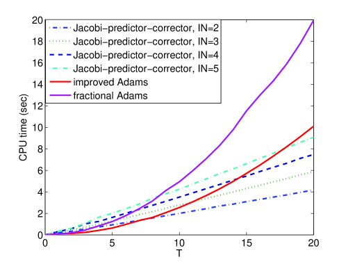
Figure 1. The CPU time needed to solve (5.1) when $\alpha=0.5,~{}h=1/40$ for the fractional Adams methods in [8], the Improved Adams methods in [4] and the Jacobi-predictor-corrector approach here when $IN=2,~{}3,~{}4,~{}5$.

Table 8 shows the CPU time (sec) and the steps $N$ needed to solve (5.1) when $\alpha=0.5$ with the maximum error $1.0\times 10^{-3}$, for the fractional Adams methods in [8], the Improved Adams methods in [4] and the Jacobi-predictor-corrector approach here when $IN=2,~{}3,~{}4,~{}5$. The consumed CPU time presented in Table 8 shows that the fractional Adams methods generates the numerical solution with the same accuracy as the other two methods, but uses much less CPU time. This advantage is more obvious as the terminate time goes long. It further demonstrates the quickness and efficiency of the Jacobi-predictor-corrector method.

Table 8. The CPU time (sec) and the steps $N$ needed to solve (5.1) when $\alpha=0.5$ with the maximum error $1.0\times 10^{-3}$, for the fractional Adams methods in [8], the Improved Adams methods in [4] and the Jacobi-predictor-corrector approach here when $IN=2,~{}3,~{}4,~{}5$.

		terminal time
methods		$T=0.5$		$T=1.0$		$T=1.5$		$T=2.0$
		$N$	CPU time (sec)	$N$	CPU time (sec)	$N$	CPU time (sec)	$N$	CPU time (sec)
fractional Adams		17	6.25 1e -2	432	5.72 1e+0	3240	3.20 1e+2	14200	6.26 1e+3
Improved Adams		14	3.13 1e -2	204	7.97 1e -1	945	1.41 1e+1	2831	1.29 1e+2
Jacobi-	$IN=2$	11	9.34 1e -2	119	6.09 1e -1	492	2.52 1e+0	1456	7.75 1e+0
predictor-	$IN=3$	7	1.56 1e -2	34	1.41 1e -1	89	5.16 1e -1	117	1.13 1e+0
corrector	$IN=4$	5	1.56 1e -2	18	7.81 1e -2	34	1.72 1e -1	51	2.97 1e -1
methods	$IN=5$	5	3.13 1e -2	13	4.69 1e -2	23	1.09 1e -1	33	1.88 1e -1

5.2. Robustness of the algorithm

Here we study the following equation as an example to show the robustness of the algorithm,

$$D^{\alpha}_{\ast}x(t)=-x(t),~{}~{}~{}~{}~{}~{}x(0)=1,~{}~{}~{}x^{\prime}(0)=0~{}~{}(\textrm{if}~{}1<\alpha\leq 2).$$ (5.3)

It is well known that the exact solution of (5.3) is

$$x(t)=E_{\alpha}(-t^{\alpha}),$$ (5.4)

where

$$E_{\alpha}(z)=\sum_{k=0}^{\infty}\frac{z^{k}}{\Gamma(\alpha k+1)},~{}~{}~{}Re(\alpha)>0,z\in\mathbb{C},$$ (5.5)

is the Mittag-Leffler function of order $\alpha$. It is obvious that neither $x(t)$ nor $D^{\alpha}_{\ast}x(t)$ has a bounded first (second) derivative at $t=0$ when $0<\alpha\leq 1$ ($1<\alpha\leq 2$), so we deal with (5.3) as we discussed in Section 4.1. Here we take $T_{0}=0.1$, $JN=26$, $\tilde{JN}=2JN$, where $T_{0},~{}JN$ and $\tilde{JN}$ are defined as in Section 4.1, and the exact solutions are calculated using the function $``mlf.m"$ [19]. The convergent order is also simply verified in Table 9 and Table 10.

Table 9. The maximum errors for (5.3) when $t\in[0,1.1]$ and $IN=2$.

h	$\alpha=0.2$	CO	$\alpha=0.5$	CO	$\alpha=1.2$	CO	$\alpha=1.8$	CO
1/10	4.84 1e-3	-	2.30 1e-3	-	1.20 1e-4	-	3.72 1e-4	-
1/20	1.49 1e-3	1.70	5.10 1e-4	2.17	3.47 1e-5	1.79	1.06 1e-4	1.81
1/40	4.04 1e-4	1.88	1.02 1e-4	2.33	7.83 1e-6	2.15	2.62 1e-5	2.02
1/80	9.96 1e-5	2.02	1.89 1e-5	2.43	1.87 1e-6	2.07	6.35 1e-6	2.05
1/160	2.44 1e-5	2.03	3.95 1e-6	2.26	5.41 1e-7	1.79	1.62 1e-6	1.97

Table 10. The maximum errors for (5.3) when $t\in[0,1.1]$ and $IN=3$.

h	$\alpha=0.2$	CO	$\alpha=0.5$	CO	$\alpha=1.2$	CO	$\alpha=1.8$	CO
1/10	2.77 1e-3	-	7.30 1e-4	-	1.11 1e-5	-	1.64 1e-5	-
1/20	6.04 1e-4	2.20	1.14 1e-4	2.68	3.23 1e-6	1.78	3.00 1e-6	2.45
1/40	1.06 1e-4	2.51	1.43 1e-5	2.99	5.48 1e-7	2.56	4.64 1e-7	2.69
1/80	1.29 1e-5	3.04	1.40 1e-6	3.36	8.88 1e-8	2.63	5.91 1e-8	2.97
1/160	1.36 1e-6	3.25	3.78 1e-8	5.21	1.09 1e-8	3.03	7.84 1e-9	2.92

Further we compute (5.3) with a big time interval, $T=50$; the parameters $IN,~{}JN,~{}\tilde{JN}$ are taken the same as the above ones and $h$ is taken as $1/10$. The exact solutions and relative errors are shown in Fig. 3 with $\alpha=0.2$ and Fig. 3 with $\alpha=0.5$. It can be seen that the relative errors in the interval are less than $O(10^{-4})$ when time is long, which suggests that our method is suitable for the long-time computation.

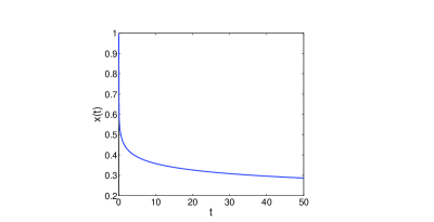
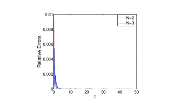
Figure 2. (a) Exact solution of (5.3) for $\alpha=0.2$; (b) Relative errors with $\alpha=0.2$, $h=1/10$, $IN=2$ or $3$.

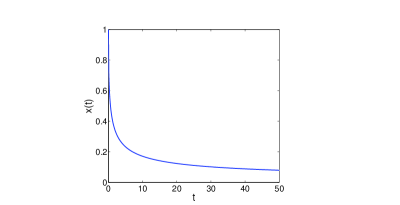
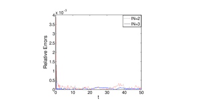
Figure 3. (a) Exact solution of (5.3) for $\alpha=0.5$; (b) Relative errors with $\alpha=0.5$, $h=1/10$, $IN=2$ or $3$.

6. Conclusion

We provide the Jacobi-predictor-corrector approach for the fractional ordinary differential equations; the basic idea is to take the Riemann-Liouville integral kernel as the Jacobi-weight function, and to realize the algorithm by doing the Jacobi-Gauss-Lobatto quadrature and polynomial interpolation. The convergent order is exactly equal to the number of interpolating nodes $IN$. The computational complexity is $O(N)$ for $\alpha\in(0,\infty)$, where $N$ is the total computational steps. This is the striking feature/advantage of the algorithm, since the computational complexity of numerically solving the fractional ordinary differential equation usually is $O(N^{2})$, caused by its nonlocal property; when $\alpha\in(0,2)$, it is possible to reduce the computational cost to $O(N\log N)$ by combining the short memory principle.

Acknowledgments. This research was supported by the Program for New Century Excellent Talents in University under Grant No. NCET-09-0438, the National Natural Science Foundation of China under Grant No. 10801067, and the Fundamental Research Funds for the Central Universities under Grant No. lzujbky-2010-63 and No. lzujbky-2012-k26. WHD thanks Chi-Wang Shu for the discussions and valuable comments.

Appendix

We display the Jacobi-Gauss-Lobatoo nodes and weighs in the reference interval $[-1,1]$ used in the numerical experiments in the following tables, where the weight function is $(1-s)^{\alpha}$, $\alpha=0.1$, $0.3$, $0.5$, $0.7$, $0.9$, $1.2$, $1.5$, $1.8$, respectively, and the number of the quadrature nodes $JN+1=27$.

Table 11.

$\alpha=0.1$		$\alpha=0.3$
nodes	weights	nodes	weights
-1.0000000000000000	0.0015793891284060	-1.0000000000000000	0.0018004451789191
-0.9892016529048960	0.0097486968513111	-0.9892836220495154	0.0111011132499144
-0.9639539701336150	0.0176099210456689	-0.9642264317182587	0.0200016826109024
-0.9247048615099546	0.0255586083473313	-0.9252701785814652	0.0289128339852526
-0.8720275885827603	0.0336423948344829	-0.8729795316392537	0.0378465851188033
-0.8066879161228238	0.0419097843832046	-0.8081088436911802	0.0468128223976810
-0.7296351534780572	0.0504145465068031	-0.7315934254809393	0.0558230223195378
-0.6419886593191621	0.0592179803160306	-0.6445363551226361	0.0648912240850699
-0.5450216478217176	0.0683915067416097	-0.5481926424422340	0.0740349165644332
-0.4401427133803333	0.0780200133502234	-0.4439511569824626	0.0832761166251512
-0.3288753760288977	0.0882063337718825	-0.3333146137264882	0.0926427678850384
-0.2128359531749780	0.0990774042058216	-0.2178779134712215	0.1021706112368920
-0.0937100816930866	0.1107929333210531	-0.0993051526697154	0.1119057485004456
0.0267717676524930	0.1235579229632447	0.0206943649229667	0.1219082421622975
0.1468594274088615	0.1376412507907670	0.1403907686322420	0.1322573016048666
0.2648084569648291	0.1534041057504351	0.2580585579193416	0.1430589703422321
0.3789054830602389	0.1713450510950583	0.3720014765729532	0.1544578938601842
0.4874930892080245	0.1921744216247991	0.4805769654678000	0.1666560217001116
0.5889938926263092	0.2169432942460124	0.5822198414675918	0.1799436799255219
0.6819334593243178	0.2472807617819305	0.6754648613490701	0.1947540530811646
0.7649617255263299	0.2858641340356679	0.7589678460750942	0.2117653286898140
0.8368726174182031	0.3374445171968009	0.8315250626755174	0.2321093791361104
0.8966215953237894	0.4113924209918509	0.8920905904778630	0.2578499674265770
0.9433409167504676	0.5293048192507985	0.9397914478954834	0.2932722023123962
0.9763527097958942	0.7555606909447271	0.9739404234643343	0.3493613894433857
0.9951835446365114	1.4176717079984273	0.9940482649436114	0.4687789976411144
1.0000000000000000	5.0539800138885518	1.0000000000000000	0.4664213940659055

Table 12.

$\alpha=0.5$		$\alpha=0.7$
nodes	weights	nodes	weights
-1.0000000000000000	0.0020525595970582	-1.0000000000000000	0.0023401106204443
-0.9893643555933919	0.0126420869565904	-0.9894438812775599	0.0143980191213123
-0.9644947993303408	0.0227208651492852	-0.9647591646875335	0.0258125839599000
-0.9258270443312571	0.0327129904967510	-0.9263756474471649	0.0370189772483234
-0.8739173433922172	0.0425872817104095	-0.8748413378464713	0.0479340538950119
-0.8095088697871018	0.0523089398061103	-0.8108884559986644	0.0584716242404765
-0.7335232176624819	0.0618432836433182	-0.7354251541586265	0.0685470018011806
-0.6470475078824108	0.0711562189729229	-0.6495229109880948	0.0780777884066716
-0.5513189009359872	0.0802144213662633	-0.5544013837390309	0.0869842827280500
-0.4477069175659654	0.0889854705911301	-0.4514111111711064	0.0951897677589023
-0.3376938533233919	0.0974379713316180	-0.3420143458160455	0.1026206972731357
-0.2228535755897699	0.1055416672643979	-0.2277642960175138	0.1092067627458629
-0.1048290089639729	0.1132675500578416	-0.1102830750128124	0.1148808056093876
0.0146913679757165	0.1205879635232249	0.0087613289573869	0.1195785218117537
0.1339976779295242	0.1274767027659907	0.1276787341676305	0.1232378787845395
0.2513831064264158	0.1339091080692547	0.2447807621576336	0.1257981209039414
0.3651683196413840	0.1398621532108058	0.3584048089141069	0.1271981640581311
0.4737254891175540	0.1453145279145870	0.4669376500627146	0.1273740449364915
0.5755015796722314	0.1502467141498365	0.5688383448113328	0.1262548372106364
0.6690405673158345	0.1546410560090228	0.6626601132252578	0.1237559426680637
0.7530042693246988	0.1584818229166975	0.7470708756553147	0.1197675894104367
0.8261914884659855	0.1617552659442731	0.8208721610920136	0.1141338609152897
0.8875551974923557	0.1644496670298319	0.8830161106263974	0.1066110258518362
0.9362175180611009	0.1665553809272196	0.9326203125145781	0.0967739548306226
0.9714822797862176	0.1680648697345029	0.9689801330973330	0.0837631042002331
0.9928449797512120	0.1689727298783471	0.9915771271381129	0.0653397616047768
1.0000000000000000	0.0846378557289007	1.0000000000000000	0.0196518498509760

Table 13.

$\alpha=0.9$		$\alpha=1.2$
nodes	weights	nodes	weights
-1.0000000000000000	0.0026680954862362	-1.0000000000000000	0.0032485813206930
-0.9895222260184334	0.0163990211169060	-0.9896375857934652	0.0199364618399667
-0.9650196167842330	0.0293282050572500	-0.9654031458102729	0.0355265819180070
-0.9269161710244489	0.0418988082171859	-0.9277121945697792	0.0504662938531113
-0.8757518197224115	0.0539656088052377	-0.8770928511031259	0.0644948884276532
-0.8122480503073657	0.0653836420874911	-0.8142509047810206	0.0773638096423790
-0.7372998407745818	0.0760144717348032	-0.7400620590862488	0.0888474771253680
-0.6519633346267486	0.0857281246221285	-0.6555600135812010	0.0987484771441300
-0.5574410233343691	0.0944045439109477	-0.5619221255221779	0.1069017533569795
-0.4550648215271042	0.1019348490180515	-0.4604530253538590	0.1131780974268036
-0.3462773061846129	0.1082224273322169	-0.3525664467804354	0.1174869327523327
-0.2326113924086162	0.1131838455110155	-0.2397655327004557	0.1197783563983938
-0.1156687346912121	0.1167495593531492	-0.1236218938939909	0.1200444135582023
0.0029028410706502	0.1188643960701240	-0.0057537131214067	0.1183195966655319
0.1214325564431927	0.1194877759976240	0.1121967999388062	0.1146805830124639
0.2382502228570740	0.1185936294194118	0.2285862886357495	0.1092452502518708
0.3517097756999029	0.1161699441834089	0.3417931453037846	0.1021710400770435
0.4602124683760809	0.1122178437862630	0.4502401041519408	0.0936527803497127
0.5622293993378423	0.1067500287515353	0.5524162161956613	0.0839201325248429
0.6563230543010921	0.0997882844987957	0.6468978998418504	0.0732349201079911
0.7411675592086939	0.0913594924131627	0.7323687733098204	0.0618887495635877
0.8155673560609422	0.0814889890869870	0.8076379911244389	0.0502016389583398
0.8784740302618931	0.0701886634133376	0.8716568246106763	0.0385230330239028
0.9290010193400755	0.0574330648431000	0.9235332376746080	0.0272382282726720
0.9664358148554766	0.0431024991510826	0.9625441648076186	0.0167880196253709
0.9902477964312976	0.0268013946767667	0.9881446058894564	0.0077265395634170
1.0000000000000000	0.0052794393153508	1.0000000000000000	0.0008846215676251

Table 14.

$\alpha=1.5$		$\alpha=1.8$
nodes	weights	nodes	weights
-1.0000000000000000	0.0039558421325122	-1.0000000000000000	0.0048176566867522
-0.9897504320058830	0.0242407262612330	-0.9898608459541634	0.0294787408291468
-0.9657783446854108	0.0430450442150069	-0.9661454822450298	0.0521665283985357
-0.9284910158577785	0.0608075612568833	-0.9292531881022244	0.0732935305513724
-0.8784051049048023	0.0771197426976410	-0.8796895020922768	0.0922636940579904
-0.8162111679198959	0.0916086237361090	-0.8181301941668921	0.1085561087536052
-0.7427661984333459	0.1039548961583067	-0.7454140912397981	0.1217534509743617
-0.6590821003162865	0.1139030192180424	-0.6625319256813679	0.1315582543475505
-0.5663118098346140	0.1212688126551674	-0.5706128999526579	0.1378033510671248
-0.4657334305951538	0.1259447610428847	-0.4709093210906420	0.1404566089311143
-0.3587326320143288	0.1279029357867882	-0.3647795460854125	0.1396198574132639
-0.2467835618430933	0.1271954603677246	-0.2536694784396956	0.1355220825893431
-0.1314285381791132	0.1239525097131300	-0.1390928704191656	0.1285072066852624
-0.0142568016179130	0.1183779081926168	-0.0226107001846948	0.1190169991802236
0.1031173793924301	0.1107424642216554	0.0941900949493554	0.1075698748132034
0.2190769482282871	0.1013752491912932	0.2097182393627444	0.0947365082759497
0.3320243383882507	0.0906530919063302	0.3223997996747073	0.0811133270750175
0.4404034835594873	0.0789886148348753	0.4306996300173916	0.0672950260065822
0.5427212564354959	0.0668171834999999	0.5331422907681873	0.0538472733927563
0.6375680414418941	0.0545831738546201	0.6283321577931673	0.0412807461037388
0.7236371592440043	0.0427259833787319	0.7149724532569940	0.0300275324422679
0.7997428790488688	0.0316662190978989	0.7918829524158366	0.0204207704286011
0.8648367821754457	0.0217924888159768	0.8580161681069255	0.0126781227682169
0.9180222971008329	0.0134491973972607	0.9124719559264060	0.0068892709351844
0.9585674487321285	0.0069256857723223	0.9545111721119047	0.0030068635217618
0.9859178863652559	0.0024466760492113	0.9835752524825214	0.0008386286076415
1.0000000000000000	0.0001742117099051	1.0000000000000000	0.0000387924881512

References

- [1] C. Canuto, M.Y. Hussaini, A. Quarteroni and T.A. Zang, Spectral Methods Fundamentals in Single Domains, Springer-Verlag, Berlin, 2006.
- [2] Y.P. Chen and T. Tang, Convergence analysis of the Jacobi spectral-collection methods for Volterra integral equations with a weakly singular kernel, Math. Comp., 79 (2010), 147-167.
- [3] V. Daftardar-Gejji and A. Babakhani, Analysis of a system of fractional differential equations, J. Math. Anal. Appl., 293 (2004), 511-522.
- [4] W.H. Deng, Numerical algorithm for the time fractional Fokker-Planck equation, J. Comp. Phys., 227 (2007), 1510-1522.
- [5] W.H. Deng, Short memory principle and a predictor-corrector aproach for fractional differential equations, J. Comput. Appl. Math., 206 (2007), 174-188.
- [6] W.H. Deng, Smoothness and stability of the solutions for nonlinear fractional differential equations, Nonl. Anal.: TMA, 72 (2010), 1768-1777.
- [7] K. Diethelm and N.J. Ford, Analysis of fractional differential equations, J. Math. Anal. Appl., 265 (2002), 229-248.
- [8] K. Diethelm, N.J. Ford and A.D. Freed, A predictor-corrector approach for the numerical solution of fractional differential eqations, Nonlinear Dynam., 29 (2002), 3-22.
- [9] K. Diethelm, N.J. Ford and A.D. Freed, Detailed error analysis for a fractional Adams method, Nonlinear Dynam., 36 (2004), 31-52.
- [10] N.J. Ford and A.C. Simpson, The numerical solution of fractional differential equations: speed versus accuracy, Numer. Algorithms, 26 (2001), 333-346.
- [11] B.Y. Guo, J. Shen and L. Wang, Optimal spectral-Galerkin methods using generalized Jacobi polynomials, J. Sci. Comput., 27 (2006), 305-322.
- [12] B.Y. Guo and L. Wang, Jacobi interpolation approximations and their applications to singular diferential equations, Adv. Comput. Math., 14 (2001), 227-276.
- [13] B.Y. Guo and L. Wang, Jacobi approximations in non-uniformly Jacobi-weighted Sobolev spaces, J. Approx. Theory, 128 (2004), 1-41.
- [14] J.S. Hesthaven, S. Gottlieb and D. Gottlieb, Spectral Methods for Time-Dependent Problems, Cambridge University Press, Cambrigde, 2007.
- [15] I. Podlubny, Fractional Differential Equations, Academic Press, New York, 1999.
- [16] A. Quarteroni, R. Sacco and F. Saleri, Numerical Mathematics, Springer-Verlag, New York, 2000.
- [17] J. Shen and T. Tang, Spectral and High-Order Methods with Applications, Science Press, Beijing, 2006.
- [18] Z.S. Wan, B.Y. Guo and Z. Q. Wang, Jacobi pseudospectral method for fourth order problems, J. Comp. Math. 24 (2006), 481-500.
- [19] http://www.mathworks.com/matlabcentral/fileexchange/8738