A New Poisson Noise Filter based on Weights Optimization

Abstract

We propose a new image denoising algorithm when the data is contaminated by a Poisson noise. As in the Non-Local Means filter, the proposed algorithm is based on a weighted linear combination of the observed image. But in contract to the latter where the weights are defined by a Gaussian kernel, we propose to choose them in an optimal way. First some ”oracle” weights are defined by minimizing a very tight upper bound of the Mean Square Error. For a practical application the weights are estimated from the observed image. We prove that the proposed filter converges at the usual optimal rate to the true image. Simulation results are presented to compare the performance of the presented filter with conventional filtering methods.

1 Introduction

In a variety of applications, ranging from nuclear medicine to night vision and from astronomy to traffic analysis, data are collected by counting a series of discrete events, such as photons hitting a detector or vehicles passing a sensor. Many such problems can be viewed as the recovery of the intensity from the indirect Poisson data. The measurements are often inherently noisy due to low count levels, and we wish to reconstruct salient features of the underlying phenomenon from these noisy measurements as accurately as possible.

There are many types of methods to reconstruct the image contaminated by the Poisson noise. The most popular method is performed through a Variance Stabilizing Transform (VST) with the following three-step procedure. First, the variance of the Poisson distribution is stabilized by applying a VST. So that the transformed data are approximately homoscedastic and Gaussian. The VST can be an Anscombe root transformation (Anscombe (ANSCOMBE1948TRANSFORMATION, ) and Borovkov (borovkov2000estimates, )), multiscal VSTs (Bardsley and Luttman (ZHANG2008WAVELETS, )), Conditional Variance Stabilization (CVS) (Jansen (jansen2006multiscale, )), or Haar-Fisz transformation (Fryzlewicz and Nason (FRYZLEWICZ2007GOES, ; FRYZLEWICZ2004HAAR, )). Second, the noise is removed using a conventional denoising algorithm for additive Gaussian white noise, see for example Buades, Coll and Morel (2005 (buades2005review, )), Kervrann (2006 (kervrann2006optimal, )), Aharon and Elad and Bruckstein (2006 (aharon2006rm, )), Hammond and Simoncelli (2008 (hammond2008image, )), Polzehl and Spokoiny (2006 (polzehl2006propagation, )), Hirakawa and Parks (2006 (hirakawa2006image, )), Mairal, Sapiro and Elad (2008 (mairal2008learning, )), Portilla, Strela, Wainwright and Simoncelli (2003 (portilla2003image, )), Roth and Black (2009 (roth2009fields, )), Katkovnik, Foi, Egiazarian, and Astola (2010 (Katkovnik2010local, )), Dabov, Foi, Katkovnik and Egiazarian (2006 (buades2009note, )), Abraham, Abraham, Desolneux and Li-Thiao-Te (2007 (Abraham2007significant, )), and Jin, Grama and Liu (2011 (JinGramaLiuowf, )). Third, an inverse transformation is applied to the denoised signal, obtaining the estimate of the signal of interest. Makitalo and Foi (2009 (MAKITALO2009INVERSION, ) and 2011 (makitalo2011optimal, )) focus on this last step, and introduce the Exact Unbiased Inverse (EUI) approach. Zhang, Fadili, and Starck (2008 (ZHANG2008WAVELETS, )), Lefkimmiatis, Maragos, and Papandreou (2009 (lefkimmiatis2009bayesian, )), Luisier, Vonesch, Blu and Unser (2010 (luisier2010fast, )) improved both the stabilization and the inverse transformation.

Regularization based on a total variation seminorm has also attracted significant attention, see for example Beck and Teboulle (2009 (beck2009fast, )), Bardsley and Luttman (2009 (bardsley2009total, )), Setzer, Steidl and Teuber (2010 (setzer2010deblurring, )). Nowak and Kolaczyk (1998 (nowak1998multiscale, ) and 2000 (nowak2000statistical, )) have investigated reconstruction algorithms specifically designed for the Poisson noise without the need of VSTs.

In this paper, we introduce a new algorithm to restore the Poisson noise without using VST’s. We combine the special properties of the Poisson distribution and the idea of Optimal Weights Filter (JinGramaLiuowf, ) for removing efficiently the Poisson noise. The use of the proposed filter is justified both from the theoretical point of view by convergence theorems, and by simulations which show that the filter is very effective.

The paper is organized as follows. Our main results are presented in Section 2 where we construct an adaptive estimator and give an estimation of its rate of convergence. In Section 3, we present our simulation results with a brief analysis. Proofs of the main results are deferred to Section 4.

2 Construction of the estimator and its convergence

2.1 The model and the notations

We suppose that the original image of the object being photographed is a integrable two-dimensional function $f(x)$, $x\in(0,1]\times(0,1]$. Let the mean value of $f$ in a set $\mathbf{B}_{x}$ be

$$\Lambda(\mathbf{B}_{x})=N^{2}\int\limits_{\mathbf{B}_{x}}f(t)dt.$$

Typically we observe a discrete data set of counts $\mathbf{Y}=\{\mathcal{N}(\mathbf{B}_{x})$}, where $\mathcal{N}(\mathbf{B}_{x})$ is a Poisson random variable of intensity $\Lambda(\mathbf{B_{x}})$. We consider that if $\mathbf{B}_{x}\cap\mathbf{B}_{y}=\emptyset,$ then $\mathcal{N}(\mathbf{B}_{x})$ is independent of $\mathcal{N}(\mathbf{B}_{y})$. For a positive integer $N$ the uniform $N\times N$ grid on the unit square is defined by

$$\mathbf{I}=\left\{\frac{1}{N},\frac{2}{N},\cdots,\frac{N-1}{N},1\right\}^{2}.$$ (1)

Each element $x$ of the grid $\mathbf{I}$ is called pixel. The number of pixels is $n=N^{2}.$ Suppose that $x=(x^{(1)},x^{(2)})\in\mathbf{I}$, and $\mathbf{B}_{x}=(x^{(1)}-1/N,x^{(1)}]\times(x^{(2)}-1/N,x^{(2)}]$. Then $\{\mathbf{B}_{x}\}_{x\in\mathbf{I}}$ is a partition of the square $(0,1]\times(0,1]$. The image function $f$ is considered to be constant on each $\mathbf{B}_{x}$, $x\in\mathbf{I}$. Hence we get a discrete function $f(x)=\Lambda(\mathbf{B}_{x})$, $x\in\mathbf{I}$. The denoising aims at estimating the underlying intensity profile $f(x)$. In the sequence we shall use the following important property of the Poisson distribution:

$$\mathbb{E}(\mathcal{N}(\mathbf{B}_{x}))=\mathbb{V}ar(\mathcal{N}(\mathbf{B}_{x}))=f(x).$$ (2)

Actually the Poisson noise model can be viewed as the following additive noise model

$$Y(x)=f(x)+\epsilon(x),$$ (3)

where

$$\epsilon(y)=Y(x)-f(x).$$ (4)

may be considered as an additive heteroscedastic noise related to the Poisson model. Due to (2), we have $\mathbb{E}(\epsilon(y))=0$ and $\mathbb{V}ar(\epsilon(y))=\mathbb{V}ar(Y(y))=f(x)$.

Let us set some notations to be used throughout the paper. The Euclidean norm of a vector $x=\left(x_{1},...,x_{d}\right)\in\mathbf{R}^{d}$ is denoted by $\left\|x\right\|_{2}=\left(\sum_{i=1}^{d}x_{i}^{2}\right)^{\frac{1}{2}}.$ The supremum norm of $x$ is denoted by $\|x\|_{\infty}=\sup_{1\leq i\leq d}\left|x_{i}\right|.$ The cardinality of a set $\mathbf{A}$ is denoted $\mathrm{card}\,\,\mathbf{A}$. For any pixel $x_{0}\in\mathbf{I}$ and a given $h>0,$ the square window

$$\mathbf{U}_{x_{0},h}=\left\{x\in\mathbf{I:\;}\|x-x_{0}\|_{\infty}\leq h\right\}$$ (5)

is called search window at $x_{0}.$ We naturally take $h$ as a multiple of $\frac{1}{N}$ ($h=\frac{k}{N}$ for some $k\in\{1,2,\cdots,N\}$). The size of the square search window $\mathbf{U}_{x_{0},h}$ is the positive integer number

$$M=(2Nh+1)^{2}=\mathrm{card}\,\ \mathbf{U}_{x_{0},h}.$$

For any pixel $x\in\mathbf{U}_{x_{0},h}$ and a given $\eta>0$. Consider a second square window $\mathbf{U}_{x,\eta}$ of size

$$m=(2N\eta+1)^{2}=\mathrm{card\ }\mathbf{U}_{x_{0},\eta}.$$

We shall call $\mathbf{U}_{x,\eta}$ local patches and $\mathbf{U}_{x,h}$ search windows. Finally, the positive part of a real number $a$ is denoted by $a^{+}$:

$$a^{+}=\left\{\begin{array}[]{cc}a&\text{if }a\geq 0,\\ 0&\text{if }a<0.\end{array}\right.$$

2.2 Construction of the estimator

Let $h>0$ be fixed. For any pixel $x_{0}\in\mathbf{I}$ consider a family of weighted estimates $\widetilde{f}_{h,w}(x_{0})$ of the form

$$\widetilde{f}_{h,w}(x_{0})=\sum_{x\in\mathbf{U}_{x_{0},h}}w(x)Y(x),$$ (6)

where the unknown weights satisfy

$$w(x)\geq 0\;\;\;\text{and\ \ \ }\sum_{x\in\mathbf{U}_{x_{0},h}}w(x)=1.$$ (7)

The usual bias and variance decomposition of the Mean Square Error gives

$$\mathbb{E}\left(\widetilde{f}_{h,w}(x_{0})-f(x_{0})\right)^{2}=Bias^{2}+Var,$$ (8)

where

$$Bias^{2}=\left(\sum_{x\in\mathbf{U}_{x_{0},h}}w(x)\left(f(x)-f(x_{0})\right)\right)^{2}$$

and

$$Var=\sum_{x\in\mathbf{U}_{x_{0},h}}w(x)^{2}f(x).$$

The decomposition (8) is commonly used to construct asymptotically minimax estimators over some given classes of functions in the nonparametric function estimation. With our approach the bias term $Bias^{2}$ will be bounded in terms of the unknown function $f$ itself. As a result we obtain some ”oracle” weights $w$ adapted to the unknown function $f$ at hand, which will be estimated further using data patches from the image $Y.$

First, we shall address the problem of determining the ”oracle” weights. With this aim denote

$$\rho(x)=\rho_{f,x_{0}}\left(x\right)=\left|f(x)-f(x_{0})\right|.$$ (9)

Note that the value of $\rho_{f,x_{0}}\left(x\right)$ characterizes the variation of the image brightness of the pixel $x$ with respect to the pixel $x_{0}.$ From the decomposition (8), we easily obtain a tight upper bound in terms of the vector $\rho_{f,x_{0}}:$

$$\mathbb{E}\left(\widetilde{f}_{h}(x_{0})-f(x_{0})\right)^{2}\leq g_{\rho_{f,x_{0}}}(w)=g_{\rho}(w),$$ (10)

where

$$g_{\rho}(w)=\left(\sum_{x\in\mathbf{U}_{x_{0},h}}w(x)\rho(x)\right)^{2}+\sum_{x\in\mathbf{U}_{x_{0},h}}w(x)^{2}f(x).$$ (11)

From the following theorem we can obtain the form of the weights $w$ which minimize the function $g_{\rho}(w)$ under the constraints (7) in terms of $\rho\left(x\right).$ For the sake of generality, we shall formulate the result for an arbitrary non-negative function $\rho(x)$, $x\in\mathbf{U}_{x,h}$, not necessarily defined by (9).

Introduce into consideration the strictly increasing function

$$M_{\rho}\left(t\right)=\sum_{x\in\mathbf{U}_{x_{0},h}}\frac{1}{f(x)}\rho(x)(t-\rho(x))^{+},\ \ \ t\geq 0.$$ (12)

Let $K_{\text{tr}}$ be the usual triangular kernel:

$$K_{\text{tr}}\left(t\right)=\left(1-\left|t\right|\right)^{+},\quad t\in\mathbf{R}^{1}.$$ (13)

Theorem 2.1

Let $\rho\left(x\right),$ $x\in\mathbf{U}_{x_{0},h}$ be an arbitrary similarity function and let $g_{\rho}(w)$ be given by (11). Suppose that $f(x)>0$ for all $x\in\mathbf{U}_{x_{0},h}$. Then there are unique weights which minimize $g_{\rho}(w)$ subject to (7), given by

$$w_{\rho}(x)=\frac{K_{\text{tr}}\left(\frac{\rho(x)}{a}\right)/f(x)}{\sum_{y\in\mathbf{U}_{x_{0},h}}K_{\text{tr}}\left(\frac{\rho(y)}{a}\right)/f(y)},$$ (14)

where $a>0$ is the unique solution of the equation

$$M_{\rho}\left(a\right)=1.$$ (15)

The proof of Theorem 2.1 is deferred to Section 4.1.

Remark 1

The bandwidth $a>0$ is the solution of

$$\sum_{x\in\mathbf{U}_{x_{0},h}}\frac{1}{f(x)}\rho(x)({a}-\rho(x))^{+}=1,$$

and can be calculated as follows. We sort the set $\{\rho(x)\,|\,x\in\mathbf{U}_{x_{0},h}\}$ in the ascending order $0=\rho_{1}\leq\rho_{2}\leq\cdots\leq\rho_{M}<\rho_{M+1}=+\infty$, where $M=\mathrm{card}\,\,\mathbf{U}_{x_{0},h}$. Let $f_{i}$ be the corresponding value of $f(x)$ (we have $f_{i}=f(x)$ if $\rho_{i}=\rho(x)$, $x\in\mathbf{U}_{x_{0},h}$). Let

$$a_{k}=\frac{1+\sum\limits_{i=1}^{k}\rho_{i}^{2}/f_{i}}{\sum\limits_{i=1}^{k}\rho_{i}/f_{i}},\quad 1\leq k\leq M,$$ (16)

and

$$k^{\ast} = \max\{1\leq k\leq M\,|\,a_{k}\geq\rho_{k}\}$$ (17)

$$= \min\{1\leq k\leq M\,|\,a_{k}<\rho_{k}\}-1,$$

with the convention that $a_{k}=\infty$ if $\rho_{k}=0$ and that $\min\varnothing=M+1$. The bandwidth $a>0$ can be expressed as ${a}=a_{k^{\ast}}$. Moreover, $k^{\ast}$ is also the unique integer $k\in\{1,\cdots,M\}$ such that $a_{k}\geq\rho_{k}$ and $a_{k+1}<\rho_{k+1}$ if $k<M$.

The proof of Remark 1 can be found in (JinGramaLiuowf, ).

Let $\rho\left(x\right),$ $x\in\mathbf{U}_{x_{0},h},$ be an arbitrary non-negative function and let $w_{\rho}$ be the optimal weights given by (14). Using these weights $w_{\rho}$ we define the family of estimates

$$f_{h}^{\ast}(x_{0})=\sum_{x\in\mathbf{U}_{x_{0},h}}w_{\rho}(x)Y(x)$$ (18)

depending on the unknown function $\rho.$ The next theorem shows that one can pick up an useful estimate from the family $f_{h}^{\ast}$ if the function $\rho$ is close to the ”true” function $\rho_{f,x_{0}}(x)=\left|f\left(x\right)-f\left(x_{0}\right)\right|,$ i.e. if

$$\rho\left(x\right)=\left|f\left(x\right)-f\left(x_{0}\right)\right|+\delta_{n},$$ (19)

where $\delta_{n}\geq 0$ is a small deterministic error. We shall prove the convergence of the estimate $f_{h}^{\ast}$ under the local Hölder condition

$$|f(x)-f(y)|\leq L\|x-y\|_{\infty}^{\beta},\,\,\,\forall x,\,y\in\mathbf{U}_{x_{0},h+\eta},$$ (20)

where $\beta>0$ is a constant, $h>0,$ $\eta>0$ and $x_{0}\in\mathbf{I}.$

In the following, $c_{i}>0$ $(i\geq 1)$ denotes a positive constant, and $O(a_{n})$ $(n\geq 1)$ denotes a sequence bounded by $c\cdot a_{n}$ for some constant $c>0$ and all $n\geq 1$. All the constants $c_{i}>0$ and $c>0$ depend only on $L$ and $\beta$; their values can be different from line to line. Let

$$\Gamma\geq\max\{f(x):x\in\mathbf{I}\}$$ (21)

be an upper bound of the image $f$.

Theorem 2.2

Assume that $h\geq c_{0}n^{-\alpha}$ with $0\leq\alpha<\frac{1}{2\beta+2}$ and $c_{0}>0,$ or that $h=c_{0}n^{-\frac{1}{2\beta+2}}$ with $c_{0}>c_{1}=\left(\Gamma\frac{\left(\beta+2\right)\left(2\beta+2\right)}{8L^{2}\beta}\right)^{\frac{1}{2\beta+2}}.$ Suppose also that the function $f>0$ satisfies the local Hölder condition (20). Let $f_{h}^{\ast}(x_{0})$ be given by (18), where the weights $w_{\rho}$ are defined by (14) and (15) with $\rho\left(x\right)=\left|f\left(x\right)-f\left(x_{0}\right)\right|+\delta_{n}$ and $\delta_{n}=O\left(n^{-\frac{\beta}{2+2\beta}}\right).$ Then

$$\mathbb{E}\left(f_{h}^{\ast}(x_{0})-f(x_{0})\right)^{2}=O\left(n^{-\frac{2\beta}{2+2\beta}}\right).$$ (22)

For the proof of this theorem see Section 4.2.

Recall that the bandwidth $h$ of order $n^{-\frac{1}{2+2\beta}}$ is required to have the optimal minimax rate of convergence $O\left(n^{-\frac{2\beta}{2+2\beta}}\right)$ of the Mean Square Error for estimating the function $f$ of local Hölder smoothness $\beta$ (cf. e.g. FanGijbels1996 ). To better understand the adaptivity property of the oracle $f_{h}^{\ast}(x_{0}),$ assume that the image $f$ at $x_{0}$ has local Hölder smoothness $\beta$ (see (Wh, )) and that $h\geq c_{0}n^{-\alpha}$ with $0\leq\alpha<\frac{1}{2\beta+2},$ which means that the radius $h>0$ of the search window $U_{x_{0},h}$ has been chosen larger than the “standard” $n^{-\frac{1}{2\beta+2}}.$ Then, by Theorem 2.2, the rate of convergence of the oracle is still of order $n^{-\frac{\beta}{2+2\beta}}$. If we choose a sufficiently large search window $U_{x_{0},h},$ then the oracle $f_{h}^{\ast}(x_{0})$ will have a rate of convergence which depends only on the unknown maximal local smoothness $\beta$ of the image $f.$ In particular, if $\beta$ is very large, then the rate will be close to $n^{-1/2},$ which ensures a good estimation of the flat regions in cases where the regions are indeed flat. More generally, since Theorem 2.2 is valid for arbitrary $\beta,$ it applies for the maximal local Hölder smoothness $\beta_{x_{0}}$ at $x_{0},$ therefore the oracle $f_{h}^{\ast}(x_{0})$ will exhibit the best rate of convergence of order $n^{-\frac{2\beta_{x_{0}}}{2+2\beta_{x_{0}}}}$ at $x_{0}.$ In other words, the procedure adapts to the best rate of convergence at each point $x_{0}$ of the image.

We justify by simulation results that the difference between the oracle $f_{h}^{\ast}$ computed with $\rho(x)=\rho_{f,x_{0}}(x)=\left|f\left(x\right)-f\left(x_{0}\right)\right|,$ and the true image $f$, is extremely small (see Table 1). This shows that, at least from the practical point of view, it is justified to optimize the upper bound $g_{\rho_{f,x_{0}}}(w)$ instead of optimizing the Mean Square Error $\mathbb{E}\left(f^{\ast}_{h}(x_{0})-f(x_{0})\right)^{2}$ itself.

The estimate $f_{h}^{*}$ with the choice $\rho\left(x\right)=\rho_{f,x_{0}}\left(x\right)$ will be called oracle filter. In particular for the oracle filter $f_{h}^{\ast},$ under the conditions of Theorem 2.2, we have

$$\mathbb{E}\left(f_{h}^{\ast}(x_{0})-f(x_{0})\right)^{2}\leq g_{\rho}\left(w_{\rho}\right)\leq cn^{-\frac{2\beta}{2+2\beta}}.$$

Now, we turn to the study of the convergence of the Optimal Weights Filter. Due to the difficulty in dealing with the dependence of the weights we shall consider a slightly modified version of the proposed algorithm: we divide the set of pixels into two disjoint parts, so that the weights are constructed from one part, and the estimation of the target function is a weighted mean along the other part. More precisely, we proceed as follows. Assume that $x_{0}\in\mathbf{I}$. Denote

$$\mathbf{I}^{\prime}_{x_{0}}=\left\{x_{0}+\left(\frac{i}{N},\frac{j}{N}\right)\in\mathbf{I}:i+j\text{ is pair }\right\},$$

and $\mathbf{I}^{\prime\prime}_{x_{0}}=\mathbf{I}\diagdown\mathbf{I}^{\prime}_{x_{0}}.$ Denote $\mathbf{U}_{x_{0},h}^{\prime}=\mathbf{U}_{x_{0},h}\cap\mathbf{I}^{\prime}_{x_{0}}$ and $\mathbf{U}_{x,\eta}^{\prime\prime}=\mathbf{U}_{x,\eta}\cap\mathbf{I}^{\prime\prime}_{x_{0}}.$ Since $\mathbf{E}|Y(x)-Y(x_{0})|^{2}=|f(x)-f(x_{0})|^{2}+f(x_{0})+f(x)$, an obvious estimate of $\mathbf{E}\left|Y(x)-Y(x_{0})\right|^{2}$ is given by

$$\frac{1}{\mathrm{card}\,\mathbf{U}^{\prime\prime}_{x_{0},\eta}}\sum_{y\in\mathbf{U}^{\prime\prime}_{x_{0},\eta}}\left|Y(y)-Y(Ty)\right|^{2},$$

where $T=T_{x_{0},x}$ is the translation mapping: $Ty=x+(y-x_{0})$. Define an estimated similarity function $\widehat{\rho}_{x_{0}}$ by

$$\widehat{\rho}_{x_{0}}(x)=\left(\left(\frac{1}{\mathrm{card}\,\mathbf{U}^{\prime\prime}_{x_{0},\eta}}\sum_{y\in{\mathbf{U}^{\prime\prime}_{x_{0},\eta}}}|Y(y)-Y(Ty)|^{2}\right)^{1/2}-\sqrt{2\overline{f}(x_{0})}\right)^{+},$$ (23)

where

$$\overline{f}(x_{0})=\frac{1}{\mathrm{card}\,\mathbf{U}^{\prime\prime}_{x_{0},\eta}}\sum_{y\in{\mathbf{U^{\prime\prime}}_{x_{0},h}}}Y(y).$$

The Optimal Weights Poisson Noise Filter (OWPNF) proposed in this paper is defined by

$$\widehat{f}_{h}(x_{0})=\sum_{x\in\mathbf{U}_{x_{0},h}^{\prime}}\widehat{w}(x)Y(x),$$ (24)

where

$$\widehat{w}=\arg\min_{w}\left(\sum_{x\in\mathbf{U}_{x_{0},h}^{\prime}}w(x)\widehat{\rho}_{x_{0}}(x,x_{0})\right)^{2}+\overline{f}(x_{0})\sum_{x\in\mathbf{U}_{x_{0},h}^{\prime}}w^{2}(x).$$ (25)

In the next theorem, we prove that with the choice $h=c_{0}n^{-\frac{1}{2\beta+2}}$ and $\eta=c_{2}n^{-\frac{1}{2\beta+2}},$ the Mean Square Error of the estimator $\widehat{f}_{h}(x_{0})$ converges nearly at the rate $n^{-\frac{2\beta}{2\beta+2}}$ which is the usual optimal rate of convergence for a given Hölder smoothness $\beta>0$ (see e.g. Fan and Gijbels (1996 (FanGijbels1996, ))).

Theorem 2.3

Assume that $h=c_{0}n^{-\frac{1}{2\beta+2}}$ with $c_{0}>c_{1}=\left(\Gamma\frac{\left(\beta+2\right)\left(2\beta+2\right)}{8L^{2}\beta}\right)^{\frac{1}{2\beta+2}}$, and that $\eta=c_{2}n^{-\frac{1}{2\beta+2}}.$ Suppose that the function $f(x)\geq\frac{1}{\ln n}$ satisfies the local Hölder condition (20). Then

$$\mathbb{E}(\widehat{f}_{h}(x_{0})-f(x_{0}))^{2}=O\left(n^{-\frac{2\beta}{2\beta+2}}\ln^{2}n\right).$$ (26)

For the proof of this theorem see Section 4.3.

3 Simulation

For simulations we use the following usual set of $256\times 256$ images: Spots$[0.08,4.99]$, Galaxy$[0,5]$, Ridges$[0.05,0.85]$, Barbara$[0.93,15.73]$ and Cells $[0.53,16.93]$ (see the first row of Figure 1). All the images are included in the package ”Denoising software for Poisson data” which can be downloaded at http://www.cs.tut.fi/ foi/invansc/. We first do the simulations with the oracle filter which shows excellent visual quality of the reconstructed image. We next present our denoising algorithm and the numerical results which are compared with related recent works ((makitalo2011optimal, ) and (ZHANG2008WAVELETS, )). Each of the aforementioned articles proposes an algorithm specifically designed for Poisson noise removal (EUI+BM3D, MS-VST + $7/9$ and MS-VST + B3 respectively).

We evaluate the performance of a denoising filter $\widehat{f}$ by using the Normalized Mean Integrated Square Error (NMISE) defined by

$$NMISE=\frac{1}{n^{\ast}}\sum_{f(x)>0,x\in\mathbf{I}}\left(\frac{(\widehat{f}(x)-f(x))^{2}}{f(x)}\right),$$

where $\widehat{f}(x)$ are the estimated intensities, $f(x)$ are the respective true vales, and $n^{\ast}=\mathrm{card}\,\{f(x):f(x)>0,x\in\mathbf{I}\}$.

3.1 Oracle Filter

In this section we present the denoising algorithm called Oracle Filter, and show its performance on some test images.

 

Algorithm: Oracle Filter

 

Repeat for each $x_{0}\in\mathbf{I}$

Let $a=1$ (give the initial value of a)

compute$\;{\rho}(x_{i})$ by (27)

reorder ${\rho}(x_{i})$ as increasing sequence

loop from $k=1$ to $M$

if $\sum_{i=1}^{k}{\rho}(x_{i})>0$

if $\frac{1+\sum_{i=1}^{k}{\rho}^{2}(x_{i})/f(x_{i})}{\sum_{i=1}^{k}\rho(x_{i})/f(x_{i})}\geq{\rho}(x_{k})$ then $a=\frac{1+\sum_{i=1}^{k}{\rho}^{2}(x_{i})/f(x_{i})}{\sum_{i=1}^{k}\rho(x_{i})/f(x_{i})}\geq{\rho}(x_{k})$

else quit loop

else continue loop

end loop

compute $w(x_{i})=\frac{(a-{\rho}(x_{i}))^{+}/f(x_{i})}{\sum_{x_{i}\in\mathbf{U}_{x_{0},h}}(a-{\rho}(x_{j}))^{+}/f(x_{j})}$

compute $f_{h}^{\ast}(x_{0})=\sum_{x_{i}\in\mathbf{U}_{x_{0},h}}w(x_{i})Y(x_{i})$.

 

We calculate the optimal weights from the original image and compute the oracle estimate from the observed image contaminated by the Poisson noise. For choosing the convenient size of the search windows, we do numerical experiments with different window sizes (see Table 1). The results show that the difference between the oracle estimator $f_{h}^{\ast}$ and the true value $f$ is extremely small. In Figure 1, the second row illustrates the visual quality of the restored images by the Oracle Filter with $M=19\times 19$. We can see that almost all the details have been retained.

Table 1: NMISE values when oracle estimator $f_{h}^{\ast}$ is applied with different values of $M$.

Size	$7\times 7$	$9\times 9$	$11\times 11$	$13\times 13$	$15\times 15$	$17\times 17$	$19\times 19$
Spots[0.08,4.99]	0.0302	0.0197	0.0166	0.0139	0.0112	0.0098	0.0104
Galaxy[0,5]	0.0284	0.0208	0.0165	0.0144	0.0122	0.0107	0.0093
Ridges[0.05,0.85]	0.0239	0.0178	0.0131	0.0109	0.0098	0.0085	0.0074
Barbara[0.93,15.73]	0.0510	0.0399	0.0304	0.0248	0.0208	0.0195	0.0174
Cells[0.53,16.93]	0.0422	0.0323	0.0257	0.0216	0.0191	0.0164	0.0146

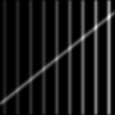
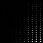
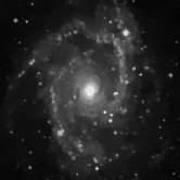
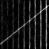
(a) Spots	(b) Galaxy	(c) Ridges	(d) Barbara	(e) Cells

Figure 1: The first row is the test images original, and the second row is the images restored by Oracle Filter with $M=19\times 19$.

3.2 Performance of the Optimal Weights Poisson Noise Filter

Throughout the simulations, we use the following algorithm for computing the Optimal Weights Poisson Noise Filter $\widehat{f}_{h}(x_{0}).$ The input values of the algorithm are $Y\left(x\right),$ $x\in\mathbf{I}$ (the image) and two numbers $m=\left(2N\eta+1\right)\times\left(2N\eta+1\right)$ and $M=\left(2Nh+1\right)\times\left(2Nh+1\right)$. In order to improve the results we introduce a smoothed version of the estimated similarity distance

$$\widehat{\rho}_{\kappa,x_{0}}(x)=\left(\sqrt{\sum_{y\in\mathbf{U}_{x_{0},\eta}}\kappa\left(y\right)\left|(Y(y)-Y(Ty)\right|^{2}}-\sqrt{2\overline{f}(x_{0})}\right)^{+},$$ (27)

where

$$\kappa\left(y\right)=\frac{K(y)}{\sum_{y^{\prime}\in\mathbf{U}_{x_{0},\eta}}K(y^{\prime})}.$$ (28)

As smoothing kernels $K(y)$ we can use the Gaussian kernel

$$K_{g}(y,h)=\exp\left(-\frac{N^{2}\|y-x_{0}\|_{2}^{2}}{2h^{2}}\right),$$ (29)

the following kernel: for $y\in\mathbf{U}_{x_{0},\eta}$,

$$K_{0}\left(y\right)=\sum_{k=\max(1,j)}^{N\eta}\frac{1}{(2k+1)^{2}}$$ (30)

if $\|y-x_{0}\|_{\infty}=\frac{j}{N}$ for some $j\in\{0,1,\cdots,N\eta\}$, and the rectangular kernel

$$K_{r}\left(y\right)=\left\{\begin{array}[]{ll}\frac{1}{\mathrm{card}\,\mathbf{U}_{x_{0},\eta}},&y\in\mathbf{U}_{x_{0},\eta},\\ 0,&\text{otherwise.}\end{array}\right.$$ (31)

The best numerical results are obtained using $K(y)=K_{0}(y)$ in the definition of $\widehat{\rho}_{\kappa,x_{0}}$. Also note that throughout the paper, we symmetrize the image near the frontier.

We present below the denoising algorithm which realizes OWPNF and shows its performance on some test images.

 

Algorithm: Optimal Weights Poisson Noise Filter (OWPNF)

 

First step:

Repeat for each $x_{0}\in\mathbf{I}$

Let $a=1$ (give the initial value of a)

compute$\;\widehat{\rho}_{\kappa,x_{0}}(x_{i})$ by (27)

reorder $\widehat{\rho}_{\kappa,x_{0}}(x_{i})$ as increasing sequence

loop from $k=1$ to $M$

if $\sum_{i=1}^{k}\widehat{\rho}_{\kappa,x_{0}}(x_{i})>0$

if $\frac{\overline{f}(x_{0})+\sum_{i=1}^{k}\widehat{\rho}_{\kappa,x_{0}}^{2}(x_{i})}{\sum_{i=1}^{k}\widehat{\rho}_{\kappa}(x_{i})}\geq\widehat{\rho}_{\kappa,x_{0}}(x_{k})$ then $a=\frac{\overline{f}(x_{0})+\sum_{i=1}^{k}\widehat{\rho}_{\kappa,x_{0}}^{2}(x_{i})}{\sum_{i=1}^{k}\widehat{\rho}_{\kappa}(x_{i})}$

else quit loop

else continue loop

end loop

compute $w(x_{i})=\frac{(a-\widehat{\rho}_{\kappa,x_{0}}(x_{i}))^{+}}{\sum_{x_{i}\in\mathbf{U}_{x_{0},h}}(a-\widehat{\rho}_{\kappa,x_{0}}(x_{j}))^{+}}$

compute $\widehat{f}^{\prime}(x_{0})=\sum_{x_{i}\in\mathbf{U}_{x_{0},h}}w(x_{i})Y(x_{i})$.

Second step:

For each $x_{0}\in\mathbf{I}$, compute $\gamma(x_{0})=\frac{1}{M}\sum_{x\in\mathbf{U}_{x_{0},h}}\widehat{f}^{\prime}(x)$

If $\gamma(x_{0})\leq 5$

compute $\widehat{f}(x_{0})=\frac{\sum_{\|x-x_{0}\|\leq d/N}K_{g}(x,H)\widehat{f}^{\prime}(x)}{\sum_{\|x-x_{0}\|\leq d/N}K_{g}(x,H)}$

else $\widehat{f}(x_{0})=\widehat{f}^{\prime}(x_{0}).$

 

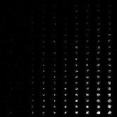
NMISE=0.0739	NMISE=0.0618	NMISE=0.0368	NMISE=0.1061	NMISE=0.0855
$M=19\times 19$	$M=15\times 15$	$M=9\times 9$	$M=15\times 15$	$M=11\times 11$
$m=13\times 13$	$m=5\times 5$	$m=19\times 19$	$m=21\times 21$	$m=17\times 17$
(a) Spots	(b) Galaxy	(c) Ridges	(d) Barbara	(e) Cells

Figure 2: These images restored by the first step of our algorithm.

Note that the presented algorithm is divided into two steps: in the first step we reconstruct the image by OWPNF from noisy data; in the second step, we smooth the image by a Gaussian kernel. This is explained by the fact that images with brightness between $0$ and $255$ (like Barbara) are well denoised by the first step, but for the low count levels images, the restored images by OWPNF are not smooth enough (see Figure 2). For these types of images, we introduce an additional smoothing using a Gaussian kernel (see the second step of the algorithm).

Our numerical experiments are done in the same way as in (ZHANG2008WAVELETS, ) and (MAKITALO2009INVERSION, ) to produce comparable results; we also use the same set of test images (all of $256\times 256$ in size): Spots $[0.08,4.99]$, Galaxy $[0,5]$, Ridges $[0.05,0.85]$, Barbara $[0.93,15.73]$, and Cells $[0.53,16.93]$. The authors of (ZHANG2008WAVELETS, ) and (MAKITALO2009INVERSION, ) kindly provided us with their programs and the test images.

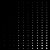
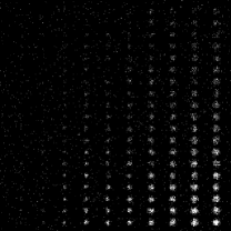
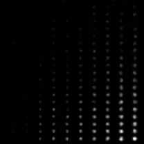
(a) Original image	(b) Noisy image	(c) OWF
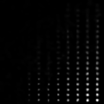
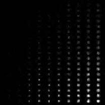
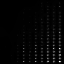
(d) EUI+BM3D	(e) MS-VST + $7/9$	(f) MS-VST + B3

Figure 3: Denoising an image of simulated spots of different radii (image size: $256\times 256$). (a) simulated sources (amplitudes $\in[0.08,4.99]$; background $=0.03$); (b) observed counts; (c) Optimal Weights Filter ($M=19\times 19$, $m=13\times 13$, $d=2$ and $H=1,$ $NMISE=0.0259$); (d) Exact unbiased inverse + BM3D ($NMISE=0.0358$) (e) MS-VST + $7/9$ biorthogonal wavelet ($J=5$, $FPR=0.01$,$N_{max}=5$ iterations, $NMISE=0.0602$); (f) MS-VST + B3 isotropic wavelet ($J=5$, $FPR=0.01$, $N_{max}=5$ iterations, $NMISE=0.81$).

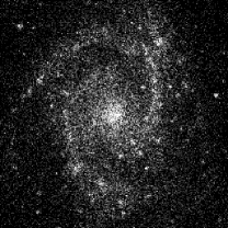
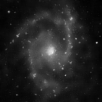
(a) Original image	(b) Noisy image	(c) OWF
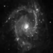
(d) EUI+BM3D	(e) MS-VST + $7/9$	(f) MS-VST + B3

Figure 4: Denoising a galaxy image (image size: $256\times 256$). (a) galaxy image (intensity $\in[0,5]$); (b) observed counts; (c) Optimal Weights Filter ($M=15\times 15$, $m=5\times 5$, $d=2$ and $H=1$, $NMISE=0.0285$); (d) Exact unbiased inverse + BM3D ($NMISE=0.0297$) (e) MS-VST + $7/9$ biorthogonal wavelet ($J=5$, $FPR=0.0001$, $N_{max}=5$ iterations, $NMISE=0.0357$); (f) MS-VST + B3 isotropic wavelet ($J=3$, $FPR=0.0001$, $N_{max}=10$ iterations, $NMISE=0.0338$).

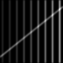
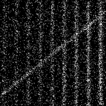
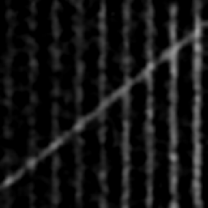
(a) Original image	(b) Noisy image	(c) OWF
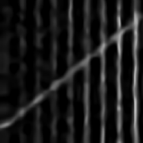
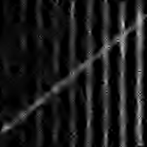
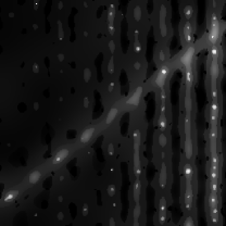
(d) EUI+BM3D	(e) MS-VST + $7/9$	(f) MS-VST + B3

Figure 5: Poisson denoising of smooth ridges (image size: $256\times 256$). (a) intensity image (the peak intensities of the $9$ vertical ridges vary progressively from $0.1$ to $0.5$; the inclined ridge has a maximum intensity of $0.3$; background $=0.05$); (b) Poisson noisy image; (c) Optimal Weights Filter ($M=9\times 9$, $m=19\times 19$, $d=3$ and $H=2$, $NMISE=0.0162$); (d) Exact unbiased inverse + BM3D ($NMISE=0.0121$); (e) MS-VST + $7/9$ biorthogonal wavelet ($J=5$, $FPR=0.001$, $N_{max}=5$ iterations, $NMISE=0.0193$); (f) MS-VST + B3 isotropic wavelet ($J=3$, $FPR=0.00001$, $N_{max}=10$ iterations, $NMISE=0.0416$).

(a) Original image	(b) Noisy image	(c) OWF
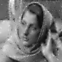
(d) EUI+BM3D	(e) MS-VST + $7/9$	(f) MS-VST + B3

Figure 6: Poisson denoising of the Barbara image (image size: $256\times 256$). (a) intensity image (intensity $\in[0.93,15.73])$; (b) Poisson noisy image; (c) Optimal Weights Filter ($M=15\times 15$, $m=21\times 21$ and $d=0$, $NMISE=0.1061$); (d) Exact unbiased inverse + BM3D ($NMISE=0.0863$) (e) MS-VST + $7/9$ biorthogonal wavelet ($J=4$, $FPR=0.001$, $N_{max}=5$ iterations, $NMISE=0.2391$); (f) MS-VST + B3 isotropic wavelet ($J=5$, $FPR=0.001$, $N_{max}=5$ iterations, $NMISE=0.3777$).

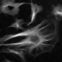
(a) Original image	(b) Noisy image	(c) OWF
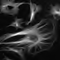
(d) EUI+BM3D	(e) MS-VST + $7/9$	(f) MS-VST + B3

Figure 7: Poisson denoising of fluorescent tubules (image size: $256\times 256$). (a) intensity image (intensity $\in[0.53,16.93])$; (b) Poisson noisy image; (c) Optimal Weights Filter ($M=11\times 11$, $m=17\times 17$, $d=1$ and $H=0.6$, $NMISE=0.0794$); (d) Exact unbiased inverse + BM3D ($NMISE=0.0643$) (e) MS-VST + $7/9$ biorthogonal wavelet ($J=5$, $FPR=0.0001$,$N_{max}=5$ iterations, $NMISE=0.0909$); (f) MS-VST + B3 isotropic wavelet ($J=5$, $FPR=0.001$, $N_{max}=10$ iterations, $NMISE=0.1487$).

Figures 3- 7 illustrate the visual quality of the denoised images using OWPNF,EUI+BM3D (makitalo2011optimal, ), MS-VST + $7/9$ (ZHANG2008WAVELETS, ), MS-VST + B3 (ZHANG2008WAVELETS, ) and PH-HMP (lefkimmiatis2009bayesian, ).

Table 2 shows the NMISE values of images reconstructed by OWPNF, EUI+BM3D, MS-VST + $7/9$, and MS-VST + B3. For Spots $[0.08,4.99]$ and Galaxy $[0,5]$, our results are the best; for Ridges $[0.05,0.85]$, Barbara $[0.93,15.73]$, and Cells $[0.53,16.93]$, the method EUI+BM3D gives the best results, but our method is also very competitive.

Algorithm	Our	EUI	MS-VST	MS-VST	PH-HMT
Algorithm	algorithm	+BM3D	+ $7/9$	+ B3
Spots$[0.08,4.99]$	$\mathbf{0.0259}$	$0.0358$	$0.0602$	$0.0810$	$0.048$
Galaxy$[0,5]$	$\mathbf{0.0285}$	$0.0297$	$0.0357$	$0.0338$	$0.030$
Ridges$[0.05,0.85]$	$0.0162$	$\mathbf{0.0121}$	$0.0193$	$0.0416$	$-$
Barbara$[0.93,15.73]$	$0.1061$	$\mathbf{0.0863}$	$0.2391$	$0.3777$	$0.159$
Cells$[0.53,16.93]$	$0.0794$	$\mathbf{0.0643}$	$0.0909$	$0.1487$	$0.082$

Table 2: Comparison between Optimal Weights Filter, MS-VST + $7/9$, and MS-VST + B3.

4 Proofs of the main results

4.1 Proof of Theorem 2.1

We begin with some preliminary results. The following lemma is similar to Theorem 1 of Sacks and Ylvisaker (Sacks1978linear, ) where, however, the inequality constraints are absent.

Lemma 1

Let $g_{\rho}(w)$ be defined by (11). Then there are unique weights $w_{\rho}$ which minimize $g_{\rho}(w)$ subject to (7), given by

$$w_{\rho}(x)=\frac{1}{f(x)}(b-\lambda\rho(x))^{+},$$ (32)

where $b$ and $\lambda$ are uniquely determined by the following two equations:

$$\sum_{x\in\mathbf{U}_{x_{0},h}}\frac{1}{f(x)}(b-\lambda\rho(x))^{+} = 1,$$ (33)

$$\sum_{x\in\mathbf{U}_{x_{0},h}}\frac{1}{f(x)}(b-\lambda\rho(x))^{+}\rho(x) = \lambda.$$ (34)

Proof

Consider the Lagrange function

$$G(w,b_{0},b)=g_{\rho}(w)-2b\left(\sum_{x\in\mathbf{U}_{x_{0},h}}w(x)-1\right)-2\sum_{x\in\mathbf{U}_{x_{0},h}}b(x)w(x),$$

where $b_{0}\in\mathbb{R}$ and $b\in\mathbb{R}^{\mathrm{card}\,\left(\mathbf{U}_{x_{0},h}\right)}$ is a vector with components $b(x)\geq 0,$ $x\in\mathbf{U}_{x_{0},h}.$ Let $w_{\rho}$ be a minimizer of $g_{\rho}\left(w\right)$ under the constraints (7). By standard results (cf. Theorem 2.2 of Rockafellar (1993 (rockafellar1993lagrange, )); see also Theorem 3.9 of Whittle (1971 (Wh, ))), there are Lagrange multipliers $b_{0}\in\mathbb{R}$ and $b(x)\geq 0,$ $x\in\mathbf{U}_{x_{0},h}$ such that the following Karush-Kuhn-Tucker conditions hold: for any $x\in\mathbf{U}_{x_{0},h},$

$$\frac{\partial}{\partial w\left(x\right)}G\left(w\right)\bigg{|}_{w=w_{\rho}}=2\lambda\rho(x)+2f(x)w_{\rho}(x)-2b-2b(x)=0,$$ (35)

with

$$\lambda=\sum_{y\in\mathbf{U}_{x_{0},h}}w_{\rho}(y)\rho(y),$$ (36)

and

$$\frac{\partial}{\partial b_{0}}G\left(w\right)\bigg{|}_{w=w_{\rho}} = \sum_{y\in\mathbf{U}_{x_{0},h}}w_{\rho}(y)-1=0,$$ (37)

$$\frac{\partial}{\partial b\left(x\right)}G\left(w\right)\bigg{|}_{w=w_{\rho}} = w_{\rho}(x)\;\left\{\begin{array}[]{cc}=0,&\text{if }b\left(x\right)>0,\\ \geq 0,&\text{if }b\left(x\right)=0.\end{array}\right.$$ (40)

(Notice that the gradients of the equality constraint function $h\left(w\right)=\sum_{x\in\mathbf{U}_{x_{0},h}}$ $w(x)-1$ and of the active inequality constraints $h_{x}\left(w\right)=w\left(x\right),$ $x\in\mathbf{U}_{x_{0},h},$ are always linearly independent, since the number of inactive inequality constraints is strictly less than $\mathrm{card}\,~{}\mathbf{U}_{x_{0},h}.$)

If $b\left(x\right)=0,$ then by (40) we have $w_{\rho}\left(x\right)\geq 0,$ so that by (35) we obtain $b-\lambda\rho(x)=f(x)w_{\rho}(x)\geq 0$ and

$$w_{\rho}(x)=\frac{(b-\lambda\rho(x))^{+}}{f(x)}.$$

If $b\left(x\right)>0,$ then by (37) we have $w_{\rho}\left(x\right)=0.$ Taking into account (35) we obtain

$$b-\lambda\rho(x)=-b(x)\leq 0,$$ (41)

so that

$$w_{\rho}(x)=0=\frac{(b-\lambda\rho(x))^{+}}{f(x)}.$$

As to conditions (33) and (34), they follow immediately from the constraint (37) and the equation (36).

Since the system (33) and (34) has a unique solution (this can be verified by substituting $\frac{b}{\lambda}=a$), the minimizer of $g_{\rho}\left(w\right)$ is also unique. The assertion of the Lemma is proved.

Now we turn to the proof of Theorem 2.1. Applying Lemma 1 with $a=b/\lambda$, we see that the unique optimal weights $w_{\rho}$ minimizing $g_{\rho}(w)$ subject to (7), are given by

$$w_{\rho}=\frac{\lambda}{f(x)}(a-\rho(x))^{+}.$$ (42)

Since the function

$$M_{\rho}(t)=\sum_{x\in\mathbf{U}_{x_{0},h}}\frac{1}{f(x)}(t-\rho(x))^{+}\rho(x)$$

is strictly increasing and continuous with $M_{\rho}(0)=0$ and $\lim\limits_{t\rightarrow\infty}M_{\rho}(a)=+\infty,$ the equation

$$M_{\rho}(a)=1$$

has a unique solution on $(0,\infty)$. The equation (34) together with (42) imply (14).

4.2 Proof of Theorem 2.2

First assume that $\rho\left(x\right)=\rho_{f,x_{0}}(x)=\left|f\left(x\right)-f\left(x_{0}\right)\right|.$ Recall that $g_{\rho}$ and $w_{\rho}$ were defined by (11) and (14). Using the Hölder condition (20) we have, for any $w$,

$$g_{\rho}(w_{\rho})\leq g_{\rho}(w)\leq\overline{g}(w),$$

where

$$\overline{g}(w)=\left(\sum_{x\in\mathbf{U}_{x_{0},h}}w(x)L\|x-x_{0}\|_{\infty}^{\beta}\right)^{2}+\Gamma\sum_{x\in\mathbf{U}_{x_{0},h}}w^{2}(x)$$ (43)

and $\Gamma$ is a constant satisfying (21). Denote $\overline{w}=\arg\min_{w}\overline{g}(w)$. Since $w_{\rho}$ minimize $g_{\rho}(w)$ and $\rho(x)\leq L\|x-x_{0}\|_{\infty}^{\beta}$, we get

$$g_{\rho}(w_{\rho})\leq g_{\rho}(\overline{w})\leq\overline{g}(\overline{w}).$$

By Theorem 2.1,

$$\overline{w}(x)=\left(\overline{a}-L\|x-x_{0}\|_{\infty}^{\beta}\right)^{+}\Big{/}\sum\limits_{x^{\prime}\in\mathbf{U}_{x_{0},h}}\left(\overline{a}-L\|x^{\prime}-x_{0}\|_{\infty}^{\beta}\right)^{+},$$ (44)

where $\overline{a}>0$ is the unique solution on $(0,\infty)$ of the equation $\overline{M}_{h}(\overline{a})=1$, where

$$\overline{{M}}_{h}\left(t\right)=\sum_{x\in\mathbf{U}_{x_{0},h}}\frac{1}{\Gamma}L\|x-x_{0}\|_{\infty}^{\beta}(t-L\|x-x_{0}\|_{\infty}^{\beta})^{+}>0.$$ (45)

Now Theorem 2.2 is a consequence of the following lemma.

Lemma 2

Assume that $\rho(x)=L\|x-x_{0}\|_{\infty}^{\beta}$ and that $h\geq c_{0}n^{-\alpha}$ with $0\leq\alpha<\frac{1}{2\beta+2}$, or $h=c_{0}n^{-\frac{1}{2\beta+2}}$ with $c_{0}\geq c_{1}\left(L,\beta\right)=\left(\frac{(2\beta+2)(\beta+2)\Gamma}{8L^{2}}\right)^{\frac{1}{2\beta+2}}.$ Then

$$\overline{a}=c_{3}n^{-\beta/(2\beta+2)}(1+o(1))$$ (46)

and

$$\overline{g}(\overline{w})\leq c_{4}n^{-\frac{2\beta}{2+2\beta}}(1+o(1)),$$ (47)

where $c_{3}$ and $c_{4}$ are constants depending only on $\beta$ and $L$.

Proof

We first prove (46) in the case where $h=1$ i.e. $\mathbf{U}_{x_{0},h}=\mathbf{I}$. In this case by the definition of $\overline{a},$ we have

$$\overline{M}_{1}\left(\overline{a}\right)=\sum\limits_{x\in\mathbf{I}}\frac{1}{\Gamma}(\overline{a}-L\|x-x_{0}\|_{\infty}^{\beta})^{+}L\|x-x_{0}\|_{\infty}^{\beta}=1.$$ (48)

Let $\overline{h}=\left(\overline{a}/L\right)^{1/\beta}$. Then $a-L\|x-x_{0}\|_{\infty}^{2}\geq 0$ if and only if $\|x-x_{0}\|\leq\overline{h}$. So from (48) we get

$$L^{2}\overline{h}^{\beta}\sum_{\|x-x_{0}\|_{\infty}\leq\overline{h}}\|x-x_{0}\|_{\infty}^{\beta}-L^{2}\sum_{\|x-x_{0}\|_{\infty}\leq\overline{h}}\|x-x_{0}\|_{\infty}^{2\beta}=\Gamma.$$ (49)

By the definition of the neighborhood $\mathbf{U}_{x_{0},\overline{h}}$, it is easily seen that

$$\sum_{\|x-x_{0}\|_{\infty}\leq\overline{h}}\|x-x_{0}\|_{\infty}^{\beta}=8N^{-\beta}\sum_{k=1}^{N\overline{h}}k^{\beta+1}=8N^{2}\frac{\overline{h}^{\beta+2}}{\beta+2}\left(1+o\left(1\right)\right)$$

and

$$\sum_{\|x-x_{0}\|_{\infty}\leq\overline{h}}\|x-x_{0}\|_{\infty}^{2\beta}=8N^{-2\beta}\sum_{k=1}^{N\overline{h}}k^{2\beta+1}=8N^{2}\frac{\overline{h}^{2\beta+2}}{2\beta+2}\left(1+o\left(1\right)\right).$$

Therefore, (49) implies

$$\frac{8L^{2}\beta}{\left(\beta+2\right)\left(2\beta+2\right)}N^{2}\overline{h}^{2\beta+2}(1+o{(1)})=\Gamma,$$

from which we infer that

$$\overline{h}=c_{1}n^{-\frac{1}{2\beta+2}}(1+o(1))$$ (50)

with $c_{1}=\left(\Gamma\frac{\left(\beta+2\right)\left(2\beta+2\right)}{8L^{2}\beta}\right)^{\frac{1}{2\beta+2}}.$ From (50) and the definition of $\overline{h}$, we obtain

$$\overline{a}=L\overline{h}^{\beta}=Lc_{1}^{\beta}n^{-\frac{\beta}{2\beta+2}}(1+o(1)),$$

which proves (46) in the case where $h=1$.

We next prove (50), which implies(46), under the conditions of the lemma. First, notice that if $\overline{h}\leq h\leq 1$, then $\overline{M}_{h}(t)=\overline{M}_{1}(t)$, $\forall t>0$. If $h\geq c_{0}n^{-\alpha},$ where $0\leq\alpha<\frac{1}{2\beta+2},$ then it is clear that $h\geq\overline{h},$ for $n$ sufficiently large. Therefore $\overline{M}_{h}\left(\overline{a}\right)=\overline{M}_{1}\left(\overline{a}\right)$, thus we arrive at the equation (48), from which we deduce (50). If $h\geq c_{0}n^{-\frac{1}{2\beta+2}}$ and $c_{0}\geq c_{1},$ then again $h\geq\overline{h}$ for $n$ sufficiently large. Therefore, $\overline{M}_{h}\left(\overline{a}\right)=\overline{M}_{1}\left(\overline{a}\right)$, and we arrive again at (50).

We finally prove (47). Denote for brevity

$$G_{h}=\sum_{\|x-x_{0}\|_{\infty}\leq h}(\overline{h}^{\beta}-\|x-x_{0}\|_{\infty}^{\beta})^{+}.$$

Since $h\geq\overline{h},$ for $n$ sufficiently large, we have $\overline{{M}}_{h}\left(\overline{a}\right)=\overline{{M}}_{\overline{h}}\left(\overline{a}\right)=1$ and $G_{h}=G_{\overline{h}}.$ Therefore by (43), (44) and (45), we get

$$\overline{g}(\overline{w}) = {\Gamma}\frac{\overline{M}_{\overline{h}}\left(\overline{a}\right)+\sum_{\|x-x_{0}\|_{\infty}\leq\overline{h}}\left(\left(\overline{a}-L\|x-x_{0}\|_{\infty}^{\beta}\right)^{+}\right)^{2}}{L^{2}G_{\overline{h}}^{2}}=\frac{{\Gamma}}{L}\frac{\overline{a}}{G_{\overline{h}}}.$$

Since

$$G_{h} =\sum_{\|x-x_{0}\|_{\infty}\leq\overline{h}}(\overline{h}^{\beta}-\|x-x_{0}\|_{\infty}^{\beta})$$

$$=\overline{h}^{\beta}\sum_{1\leq k\leq N\overline{h}}8k-\frac{8}{N^{\beta}}\sum_{1\leq k\leq N\overline{h}}k^{\beta+1}$$

$$=\frac{4\beta}{\beta+2}N^{2}\overline{h}^{\beta+2}\left(1+o\left(1\right)\right)$$

$$=\frac{4\beta}{\left(\beta+2\right)L^{1/\beta}}N^{2}\overline{a}^{\left(\beta+2\right)/\beta}\left(1+o\left(1\right)\right),$$

we obtain

$$\overline{g}\left(\overline{w}\right)=\Gamma\frac{\left(\beta+2\right)}{4\beta}L^{1/\beta-1}\frac{\overline{a}^{-\frac{2}{\beta}}}{N^{2}}\left(1+o\left(1\right)\right)\leq c_{4}n^{-\frac{2\beta}{2\beta+2}}\left(1+o\left(1\right)\right),$$

where $c_{4}$ is a constant depending on $\beta$ and $L$.

Proof of Theorem 2.2. As $\rho\left(x\right)=\left|f\left(x\right)-f\left(x_{0}\right)\right|+\delta_{n},$ we have

$$\begin{split}\left(\sum_{x\in\mathbf{U}_{x_{0},h}}w(x)\rho(x)\right)^{2}&\leq\left(\sum_{x\in\mathbf{U}_{x_{0},h}}w(x)|f(x)-f(x_{0})|+\delta_{n}\right)^{2}\\ &\leq 2\left(\sum_{x\in\mathbf{U}_{x_{0},h}}w(x)|f(x)-f(x_{0})|\right)^{2}+2\delta_{n}^{2}.\end{split}$$

Since $f(x)\leq\Gamma,$ with $g_{\rho}$ and $\overline{g}$ by (11) and (43), we get

$$g_{\rho}(w)\leq 2\overline{g}(w)+2\delta_{n}^{2}.$$

So

$$g_{\rho}(w_{\rho})\leq g_{\rho}(\overline{w})\leq 2\overline{g}(\overline{w})+2\delta_{n}^{2}.$$

Therefore, by Lemma 2 and the condition that $\delta_{n}=O\left(n^{-\frac{\beta}{2\beta+2}}\right)$, we obtain

$$g_{\rho}(w_{\rho})=O\left(n^{-\frac{2\beta}{2\beta+2}}\right).$$

This together with (10) give (22).

4.3 Proof of Theorem 2.3

Let $M^{\prime}=\mathrm{card}\,\mathbf{U}_{x_{0},h}^{\prime}=(2Nh+1)^{2}/2$, $m^{\prime}=\mathrm{card}\,\mathbf{U}^{\prime\prime}_{x_{0},\eta}=(2N\eta+1)^{2}/2$. Denote $\Delta_{x_{0},x}\left(y\right)=f(y)-f(Ty)$ and $\eta\left(y\right)=\epsilon(y)-\epsilon(Ty)$, where $\epsilon$ is defined by (4). It is easy to see that

$$\frac{1}{m^{\prime}}\sum_{y\in\mathbf{U}^{\prime\prime}_{x_{0},\eta}}\left(Y(y)-Y(Ty)\right)^{2}=\frac{1}{m^{\prime}}\sum_{y\in\mathbf{U}^{\prime\prime}_{x_{0},\eta}}\Delta^{2}_{x_{0},x}\left(y\right)+\frac{1}{m^{\prime}}S(x)+\overline{f}(x_{0})+\overline{f}(x),$$

where $S(x)=S_{2}(x)-S_{1}(x),$ with

$$S_{1}(x) = 2\sum_{y\in\mathbf{U}^{\prime\prime}_{x_{0},\eta}}\Delta_{x_{0},x}\left(y\right)\eta\left(y\right),$$

$$S_{2}(x) = \sum_{y\in\mathbf{U}^{\prime\prime}_{x_{0},\eta}}\left(\eta^{2}\left(y\right)-\overline{f}(x_{0})-\overline{f}(x)\right).$$

Denote

$$V=\frac{1}{m^{\prime}}\sum_{y\in\mathbf{U}^{\prime\prime}_{x_{0},\eta}}\Delta^{2}_{x_{0},x}\left(y\right)+\frac{1}{m^{\prime}}S(x).$$

Then

$$\begin{split}\widehat{\rho}_{x_{0}}(x)&=\left(\sqrt{V+\overline{f}(x_{0})+\overline{f}(x)}-\sqrt{2\overline{f}(x_{0})}\right)^{+}\\ &\leq\left|\sqrt{V+\overline{f}(x_{0})+\overline{f}(x)}-\sqrt{2\overline{f}(x_{0})}\right|.\end{split}$$ (51)

Using one-term Taylor expansion, we obtain

$$\begin{split}&\left|\sqrt{V+\overline{f}(x_{0})+\overline{f}(x)}-\sqrt{2\overline{f}(x_{0})}\right|\\ &\leq\frac{|V|}{(\overline{f}(x_{0})+\overline{f}(x)+\theta V)^{1/2}}+\left|\sqrt{\overline{f}(x_{0})+\overline{f}(x)}-\sqrt{2\overline{f}(x_{0})}\right|\\ &\leq\frac{\frac{1}{m^{\prime}}\sum_{y\in\mathbf{U}^{\prime\prime}_{x_{0},\eta}}\Delta^{2}_{x_{0},x}(y)+\frac{1}{m^{\prime}}|S(x)|}{(\overline{f}(x_{0})+\overline{f}(x)+\theta V)^{1/2}}+\left|\frac{\overline{f}(x)-\overline{f}(x_{0})}{\sqrt{\overline{f}(x_{0})+\overline{f}(x)}+\sqrt{2\overline{f}(x_{0})}}\right|.\end{split}$$ (52)

Since $f(x)\geq 1/\ln n$, $x\in\mathbf{I}$, (51) and (52) imply that

$$\widehat{\rho}_{x_{0}}(x)\leq\frac{L^{2}h^{2\beta}+\frac{1}{m^{\prime}}|S(x)|}{(2/\ln n+\theta V)^{1/2}}+c_{3}h\sqrt{\ln n}.$$ (53)

We shall use three lemmas to finish the Proof of Theorem 2.3.

The following lemma can be deduced form the results in Borovkov (borovkov2000estimates, ), see also Merlevede, Peligrad and Rio (merlev de2010bernstein, ).

Lemma 3

If, for some $\delta>0,\gamma\in(0,1)$ and $K>1$ we have

$$\sup\mathbb{E}\exp\left(\delta\left|X_{i}\right|^{\gamma}\right)\leq K,\;i=1,...,n,$$

then there are two positive constants $c_{1}$ and $c_{2}$ depending only on $\delta,$ $\gamma$ and $K$ such that, for any $t>0,$

$$\mathbb{P}\left(\sum_{i=1}^{n}X_{i}\geq t\right)\leq\exp\left(-c_{1}t^{2}/n\right)+n\exp\left(-c_{2}t^{\gamma}\right).$$

Lemma 4

Assume that $h=c_{0}n^{-\frac{1}{2\beta+2}}$ with $c_{0}>c_{1}=\left(\Gamma\frac{\left(\beta+2\right)\left(2\beta+2\right)}{8L^{2}\beta}\right)^{\frac{1}{2\beta+2}}$ and that $\eta=c_{2}n^{-\frac{1}{2\beta+2}}.$ Suppose that the function $f$ satisfies the local Hölder condition (20). Then there exists a constant $c_{4}>0$ depending only on $\beta$ and $L$, such that

$$\mathbb{P}\left\{\max_{x\in\mathbf{U}^{\prime}_{x_{0},h}}\widehat{\rho}_{x_{0}}(x)\geq c_{4}n^{-\frac{\beta}{2\beta+2}}\sqrt{\ln n}\right\}=O\left(n^{-\frac{2\beta}{2\beta+2}}\right).$$ (54)

Proof

Note that

$$\mathbb{E}e^{Y(y)}=\sum_{k=0}^{+\infty}e^{k}\frac{f^{k}(x)e^{-f(x)}}{k!}=ef(y)e^{(e-1)f(y)}\leq e\Gamma e^{(e-1)\Gamma}.$$

From this inequality we easily deduce that

$$\sup_{y}\mathbb{E}\left(e^{|Z(y)|^{1/2}}\right) \leq \sup_{y}\left(\mathbb{E}e^{Y(T_{x,x_{0}}y)+Y(y)+\sqrt{2(\Gamma^{2}+\Gamma)}}\right)$$

$$\leq \left(e\Gamma\right)^{2}e^{2(e-1)\Gamma+\sqrt{2(\Gamma^{2}+\Gamma)}},$$

where

$$Z(y)=2\Delta_{x_{0},x}\left(y\right)\eta\left(y\right)+\left(\eta^{2}\left(y\right)-\overline{f}(x_{0})-\overline{f}(x)\right).$$

By Lemma 3, we infer that there exists two positive constants $c_{5}$ and $c_{6}$ such that

$$\mathbb{P}\left(\frac{1}{m^{\prime}}|S(x)|\geq z/\sqrt{m^{\prime}}\right)\leq\exp(-c_{5}z^{2})+m^{\prime}\exp(-c_{6}(\sqrt{m^{\prime}}z)^{\frac{1}{2}}).$$ (55)

Substituting $z=\sqrt{\frac{1}{c_{5}}\ln m^{\prime}M^{\prime}}$ into the inequality (55), we see that for $m^{\prime}$ large enough,

$$\mathbb{P}\left(\frac{1}{m^{\prime}}\left|S(x)\right|\geq\frac{\sqrt{\frac{1}{c_{5}}\ln m^{\prime}M^{\prime}}}{\sqrt{m^{\prime}}}\right)\leq 2\exp\left(-\ln m^{\prime}M^{\prime}\right)=\frac{2}{m^{\prime}M^{\prime}}.$$

From this inequality we easily deduce that

$$\mathbb{P}\left(\max_{x\in\mathbf{U}_{x_{0},h}^{\prime}}\frac{1}{m^{\prime}}\left|S(x)\right|\geq\frac{\sqrt{\frac{1}{c_{5}}\ln m^{\prime}M^{\prime}}}{\sqrt{m^{\prime}}}\right)$$

$$\leq \sum_{x\in\mathbf{U}_{x_{0},h}^{\prime}}\mathbb{P}\left(\frac{1}{m^{\prime}}\left|S(x)\right|\geq\frac{\sqrt{\frac{1}{c_{5}}\ln m^{\prime}M^{\prime}}}{\sqrt{m^{\prime}}}\right)\leq\frac{2}{m^{\prime}}.$$

Taking $M^{\prime}=(2Nh+1)^{2}/2=c_{0}^{2}n^{\frac{2\beta}{2\beta+2}}/2$ and $m^{\prime}=(2N\eta+1)^{2}/2=c_{2}^{2}n^{\frac{2\beta}{2\beta+2}}/2$, we arrive at

$$\mathbb{P}\left(\mathbf{B}\right)\leq c_{7}n^{-\frac{2\beta}{2\beta+2}},$$ (56)

where $\mathbf{B}=\{\max_{x\in\mathbf{U}_{x_{0},h}^{\prime}}\frac{1}{m^{\prime}}\left|S(x)\right|\geq c_{8}n^{-\frac{\beta}{2\beta+2}}\sqrt{\ln n}\}$ and $c_{8}$ is a constant depending only on $\beta$ and $L$. Since on the set $\mathbf{B}$ we have

$$\left(\frac{2}{\ln n}+\theta V\right)^{1/2}<\frac{1}{\sqrt{\ln n}}$$ (57)

for $n$ large enough, combining (53), (56) and (57), we get (54).

Lemma 5

Suppose that the conditions of Theorem 2.3 are satisfied. Then

$$\mathbb{P}\left(\mathbb{E}\{|\widehat{f}_{h}(x_{0})-f(x_{0})|^{2}\big{|}Y(x),x\in\mathbf{I}^{\prime\prime}_{x_{0}}\}\geq c_{9}n^{-\frac{2\beta}{2\beta+2}}\ln n\right)=O(n^{-\frac{2\beta}{2\beta+2}}),$$

where $c_{9}>0$ is a constant depending only on $\beta$ and $L$.

Proof

Taking into account (23), (24) and the independence of $\epsilon(x)$, we have

$$\begin{split}&\mathbb{E}\{|\widehat{f}_{h}(x_{0})-f(x_{0})|^{2}\big{|}Y(x),x\in\mathbf{I}^{\prime\prime}_{x_{0}}\}\\ &\leq\left(\sum_{x\in\mathbf{U}_{x_{0},h(x)}^{\prime}}\widehat{w}(x)\rho(x)\right)^{2}+\overline{f}(x)\sum_{x\in\mathbf{U}_{x_{0},h(x)}^{\prime}}\widehat{w}^{2}(x).\end{split}$$ (58)

Since $\rho(x)<Lh^{\beta}$, from (58) we get

$$\begin{split}&\mathbb{E}\{|\widehat{f}_{h}(x_{0})-f(x_{0})|^{2}\big{|}Y(x),x\in\mathbf{I}^{\prime\prime}_{x_{0}}\}\\ &\leq\left(\sum_{x\in\mathbf{U}_{x_{0},h}^{\prime}}\widehat{w}(x)Lh^{\beta}\right)^{2}+\overline{f}(x)\sum_{x\in\mathbf{U}_{x_{0},h}^{\prime}}\widehat{w}^{2}(x)\\ &\leq\left(\left(\sum_{x\in\mathbf{U}_{x_{0},h}^{\prime}}\widehat{w}(x)\widehat{\rho}_{x_{0}}(x)\right)^{2}+\overline{f}(x)\sum_{x\in\mathbf{U}_{x_{0},h}^{\prime}}\widehat{w}^{2}(x)\right)+L^{2}h^{2\beta}.\end{split}$$

Recall that $\widehat{w}(x)$ stand for the optimal weights, defined by (25). Therefore

$$\begin{split}&\mathbb{E}\{|\widehat{f}_{h}(x_{0})-f(x_{0})|^{2}\big{|}Y(x),x\in\mathbf{I}^{\prime\prime}_{x_{0}}\}\\ &\leq\left(\left(\sum_{x\in\mathbf{U}_{x_{0},h}^{\prime}}{\overline{w}}_{1}(x)\widehat{\rho}_{x_{0}}(x)\right)^{2}+\overline{f}(x)\sum_{x\in\mathbf{U}_{x_{0},h}^{\prime}}{\overline{w}}_{1}^{2}(x)\right)+L^{2}h^{2\beta},\end{split}$$ (59)

where $\overline{w}_{1}=\arg\min\limits_{w}\overline{g}_{1}(w)$ with

$$\overline{g}_{1}(w)=\left(\sum_{x\in\mathbf{U}_{x_{0},h}^{\prime}}{w}(x)L\|x-x_{0}\|_{\infty}^{\beta}\right)^{2}+\Gamma\sum_{x\in\mathbf{U}_{x_{0},h}^{\prime}}{w}^{2}(x).$$

Since by Lemma 4,

$$\mathbb{P}\left\{\max_{x\in\mathbf{U}_{x_{0},h}}\widehat{\rho}_{x_{0}}(x)<c_{4}n^{-\frac{\beta}{2\beta+2}}\sqrt{\ln n}\right\}=1-O(n^{-\frac{2\beta}{2\beta+2}}),$$

the inequality (59) becomes

$$\begin{split}&\mathbb{P}\left(\mathbb{E}\{|\widehat{f}_{h}(x_{0})-f(x_{0})|^{2}\big{|}Y(x),x\in\mathbf{I}^{\prime\prime}_{x_{0}}\}<\overline{g}_{1}(\overline{w}_{1})+2c^{2}_{4}n^{-\frac{2\beta}{2\beta+2}}\ln n+L^{2}h^{2\beta}\right)\\ &=1-O(n^{-\frac{2\beta}{2\beta+2}}).\end{split}$$

Now, the assertion of the theorem is obtained easily if we note that $h^{2\beta}=c_{10}^{2\beta}n^{-\frac{2\beta}{2\beta+2}}$ and $\overline{g}_{1}(\overline{w}_{1})\leq c_{11}n^{-\frac{2\beta}{2\beta+2}},$ for some constant $c_{12}$ depending only on $\beta$ and $L$ (by Lemma 2 with $\mathbf{U}_{x_{0},h}^{\prime}$ instead of $\mathbf{U}_{x_{0},h}$).

Proof of Theorem 2.3. Using (58), the condition (20) and bound $f(x)\leq\Gamma$ we obtain

$$\mathbb{E}\left(|\widehat{f}_{h}(x_{0})-f(x_{0})|^{2}\big{|}Y(x),x\in\mathbf{I}^{\prime\prime}_{x_{0}},\right)\leq\overline{g}_{1}(\widehat{w})\leq c_{12},$$

for a constant $c_{14}>0$ depending only on $\beta$, $L$ and $\Gamma$. Applying Lemma 5, we have

$$\begin{split}\mathbb{E}&\left(|\widehat{f}_{h}(x_{0})-f(x_{0})|^{2}\big{|}Y(x),x\in\mathbf{I}^{\prime\prime}_{x_{0}},\right)\\ <&\mathbb{P}\left(E\{|\widehat{f}_{h}(x_{0})-f(x_{0})|^{2}\big{|}Y(x),x\in\mathbf{I}^{\prime\prime}_{x_{0}}\}<c_{9}n^{-\frac{2\beta}{2\beta+2}}\ln n\right)c_{9}n^{-\frac{2\beta}{2\beta+2}}\ln n\\ &+\mathbb{P}\left(E\{|\widehat{f}_{h}(x_{0})-f(x_{0})|^{2}\big{|}Y(x),x\in\mathbf{I}^{\prime\prime}_{x_{0}}\}\geq c_{9}n^{-\frac{2\beta}{2\beta+2}}\ln n\right)c_{12}\\ =&O\left(n^{-\frac{2\beta}{2\beta+2}}\ln n\right),\end{split}$$

where the constant in $O$ depending only on $\beta$, $L$ and $\Gamma$. Taking expectation proves Theorem 2.3.

References

- (1) Abraham, I., Abraham, R., Desolneux, A., and Li-Thiao-Te, S. : Significant edges in the case of non-stationary gaussian noise. Pattern recognition, 40(11):3277–3291 (2007)
- (2) Aharon, M., Elad, M., and Bruckstein, A. : -svd: An algorithm for designing overcomplete dictionaries for sparse representation. IEEE Trans. Signal Process., 54(11):4311–4322(2006)
- (3) Anscombe, F. : The transformation of poisson, binomial and negative-binomial data. Biometrika, 35(3/4):246–254(1948)
- (4) Bardsley, J. and Luttman, A. : Total variation-penalized poisson likelihood estimation for ill-posed problems. Adv. Comput. Math., 31(1):35–59(2009)
- (5) Beck, A. and Teboulle, M. : Fast gradient-based algorithms for constrained total variation image denoising and deblurring problems. IEEE Trans. Image Process., 18(11):2419–2434(2009)
- (6) Borovkov, A. : Estimates for the distribution of sums and maxima of sums of random variables without the cramer condition. Siberian Mathematical Journal, 41(5):811–848(2000)
- (7) Buades, A., Coll, B., and Morel, J. : A review of image denoising algorithms, with a new one. Multiscale Model. Simul., 4(2):490–530(2005)
- (8) Buades, T., Lou, Y., Morel, J., and Tang, Z. : A note on multi-image denoising. In Int. workshop on Local and Non-Local Approximation in Image Processing, pages 1–15(2009)
- (9) Fan, J. and Gijbels, I.: Local polynomial modelling and its applications. In Chapman & Hall, London (1996)
- (10) Fryzlewicz, P., Delouille, V., and Nason, G.: Goes-8 x-ray sensor variance stabilization using the multiscale data-driven haar–fisz transform. J. Roy. Statist. Soc. ser. C, 56(1):99–116 (2007)
- (11) Fryzlewicz, P. and Nason, G.: A haar-fisz algorithm for poisson intensity estimation. J. Comp. Graph. Stat., 13(3):621–638 (2004)
- (12) Hammond, D. and Simoncelli, E.: Image modeling and denoising with orientation-adapted gaussian scale mixtures. IEEE Trans. Image Process., 17(11):2089–2101 (2008)
- (13) Hirakawa, K. and Parks, T.: Image denoising using total least squares. IEEE Trans. Image Process., 15(9):2730–2742 (2006)
- (14) Jansen, M.: Multiscale poisson data smoothing. J. Roy. Statist. Soc. B, 68(1):27–48 (2006)
- (15) Jin, Q., Grama, I., and Liu, Q.: Removing gaussian noise by optimization of weights in non-local means. http://arxiv.org/abs/1109.5640.
- (16) Katkovnik, V., Foi, A., Egiazarian, K., and Astola, J.: From local kernel to nonlocal multiple-model image denoising. Int. J. Comput. Vis., 86(1):1–32 (2010)
- (17) Kervrann, C. and Boulanger, J.: Optimal spatial adaptation for patch-based image denoising. IEEE Trans. Image Process., 15(10):2866–2878 (2006)
- (18) Lefkimmiatis, S., Maragos, P., and Papandreou, G.: Bayesian inference on multiscale models for poisson intensity estimation: Applications to photon-limited image denoising. IEEE Trans. Image Process., 18(8):1724–1741 (2009)
- (19) Luisier, F., Vonesch, C., Blu, T., and Unser, M.: Fast interscale wavelet denoising of poisson-corrupted images. Signal Process., 90(2):415–427 (2010)
- (20) Mairal, J., Sapiro, G., and Elad, M.: Learning multiscale sparse representations for image and video restoration. SIAM Multiscale Modeling and Simulation, 7(1):214–241 (2008)
- (21) Makitalo, M. and Foi, A.: On the inversion of the anscombe transformation in low-count poisson image denoising. In Proc. Int. Workshop on Local and Non-Local Approx. in Image Process., LNLA 2009, Tuusula, Finland, pages 26–32. IEEE (2009)
- (22) Makitalo, M. and Foi, A.: Optimal inversion of the anscombe transformation in low-count poisson image denoising. IEEE Trans. Image Process., 20(1):99–109 (2011)
- (23) Merlevède, F., Peligrad, M., and Rio, E.: A bernstein type inequality and moderate deviations for weakly dependent sequences. Probab. Theory Related Fields (2010)
- (24) Nowak, R. and Kolaczyk, E.: A multiscale map estimation method for poisson inverse problems. In in 32nd Asilomar Conf. Signals, Systems, and Comp., volume 2, pages 1682–1686 (1998)
- (25) Nowak, R. and Kolaczyk, E.: A statistical multiscale framework for poisson inverse problems. IEEE Trans. Info. Theory, 46(5):1811–1825 (2000)
- (26) Polzehl, J. and Spokoiny, V.: Propagation-separation approach for local likelihood estimation. Probab. Theory Rel., 135(3):335–362 (2006)
- (27) Portilla, J., Strela, V., Wainwright, M., and Simoncelli, E.: Image denoising using scale mixtures of gaussians in the wavelet domain. IEEE Trans. Image Process., 12(11):1338–1351 (2003)
- (28) Rockafellar, R.: Lagrange multipliers and optimality. SIAM review, pages 183–238 (1993)
- (29) Roth, S. and Black, M.: Fields of experts. Int. J. Comput. Vision, 82(2):205–229 (2009)
- (30) Sacks, J. and Ylvisaker, D.: Linear estimation for approximately linear models. Ann. Stat., 6(5):1122–1137 (1978)
- (31) Setzer, S., Steidl, G., and Teuber, T. : Deblurring poissonian images by split bregman techniques. J. Visual Commun. Image Represent., 21(3):193–199 (2010)
- (32) Whittle, P. : Optimization under constraints: theory and applications of nonlinear programming. In Wiley-Interscience, New York (1971)
- (33) Zhang, B., Fadili, J., and Starck, J. : Wavelets, ridgelets, and curvelets for poisson noise removal. IEEE Trans. Image Process., 17(7):1093–1108 (2008)