Matching of analytical and numerical solutions for neutron stars of arbitrary rotation

Abstract

We demonstrate the results of an attempt to match the two-soliton analytical solution with the numerically produced solutions of the Einstein field equations, that describe the spacetime exterior of rotating neutron stars, for arbitrary rotation. The matching procedure is performed by equating the first four multipole moments of the analytical solution to the multipole moments of the numerical one. We then argue that in order to check the effectiveness of the matching of the analytical with the numerical solution we should compare the metric components, the radius of the innermost stable circular orbit ($R_{ISCO}$), the rotation frequency $\Omega\equiv\frac{d\phi}{dt}$ and the epicyclic frequencies $\Omega_{\rho},\;\Omega_{z}$. Finally we present some results of the comparison.

1 Introduction

Obtaining the geometry of the spacetime that surrounds a rotating distribution of mass in an exact form, is a problem of astrophysical relevance that remains unsolved. When modelling the astrophysical phenomena that we observe around rotating neutron stars, there are only a few choices we can make for the geometry we will use. We can either use one of the very well understood geometries of Schwarzschild or Kerr, which can only be used as very rough approximations, or we have to use a numerically obtained spacetime.

Although there are various groups (see [1], and for an extended list of numerical schemes see [2]), that have expertise in building relativistic models of astrophysical objects with adjustable physical characteristics and can construct the metric inside and outside such objects by solving numerically the full Einstein equations in stationary cases, having the metric of the spacetime in tabulated form with numerical values that correspond to the metric components at a selected grid is not always appropriate for studying the phenomena around the object.

Thus, an analytical solution that could describe the geometry around such an object would be useful. Fortunately, nowadays, there is a large variety of analytical solutions of vacuum Einstein equations, which could be used as candidate metrics to describe well the exterior space-time of axisymmetric astrophysical objects. Ernst [3] formulated the Einstein equations in the case of axisymmetric stationary space-times long time ago, while Manko et al. and Sibgatullin [4, 5, 6, 7, 8, 9] have used various analytical methods to produce such spacetimes parameterized by various parameters that have a different physical context depending on the type of each solution.

Such an analytical solution, appropriately matched to a neutron star, could be used to describe the stationary properties of the spacetime. That is, study the geodesics in the exterior of the neutron star. In other words, from the analytical solution, we could obtain bounds of motion for test particles, the location of the innermost stable circular orbit (ISCO), the rotation frequency of the circular orbits on the equatorial plane as well as the epicyclic frequencies around them.

These properties that are of astrophysical relevance and characteristic of a spacetime, will be used to compare the proposed analytical solution to the numerically produced solutions that describe the spacetime exterior to a neutron star.

The rest of the paper is organized as follows: In Sec. 2 the proposed analytical solution (two-soliton) is briefly presented and some of its properties analyzed. In Sec. 3 we present at first the matching criteria and then the comparison criteria and some results.

2 An Analytical axially symmetric solution: The Two Soliton solution.

The vacuum region of a stationary and axially symmetric spacetime can be described by the Papapetrou line element [10]

$$ds^{2}=-f\left(dt-\omega d\phi\right)^{2}+f^{-1}\left[e^{2\gamma}\left(d\rho^{2}+dz^{2}\right)+\rho^{2}d\phi^{2}\right],$$ (1)

were the functions $f,\;\omega$ and $\gamma$ are functions of the Weyl-Papapetrou coordinates ($\rho,\;z$). Using this metric, the Einstein field equations in vacuum reduce to the Ernst equation [3]

$$Re(\mathcal{E})\nabla^{2}\mathcal{E}=\nabla\mathcal{E}\cdot\nabla\mathcal{E},$$ (2)

were the Ernst potential $\mathcal{E},$ is a complex function of the metric functions.

A general procedure for generating solutions of the Ernst equation was developed by Sibgatullin and Manko [8, 9, 6, 4]. The solution of the Ernst equation is produced from a choice of the Ernst potential on the axis of the form

$$\mathcal{E}(\rho=0,z)=e(z)=\frac{P(z)}{R(z)},$$ (3)

were the functions $P(z),R(z)$ are polynomials of order $n$ with complex coefficients in general. In [6], one can find a detailed description of the procedure for generating the solutions using the parameters of the Ernst potential. It is shown in [6] that the metric functions are finally expressed in terms of some determinants, which depend on the parameters $\xi_{n}$, which are the $2n$ roots of the equation $e(z)+e(z)^{*}=0$, the parameters $e_{n},\;f_{n}$ and $\beta_{n}$, which are defined from the expressions

$$e(z)=1+\sum^{n}_{k=1}\frac{e_{k}}{z-\beta_{k}},\;\;f(z)=\sum^{n}_{k=1}\frac{f_{k}}{z-\beta_{k}}$$

and finally the expressions $R_{n}=\sqrt{\rho^{2}+(z-\xi_{n})^{2}}$, which are functions of the coordinates $(\rho,z)$.

The vacuum two-soliton solution (proposed by Manko [4]) is a special case of the previous general axisymmetric solution that is obtained from the ansatz (see also [11])

$$e(z)=\frac{(z-M-ia)(z+ib)-k}{(z+M-ia)(z+ib)-k}$$ (4)

where all the parameters are real while the parameters $M,\;a$ are the mass and the reduced angular momentum $\frac{J}{M}$ respectively. The first five mass and angular momentum moments of the corresponding spacetime are:

$$M_{0} = M,\quad M_{1}=0,\quad M_{2}=-(a^{2}-k)M,\quad M_{3}=0,$$

$$M_{4} = \left(a^{4}-(3a^{2}-2ab+b^{2})k+k^{2}+\frac{1}{7}(2a^{2}-k)M^{2}\right)M$$

$$J_{0} = 0,\quad J_{1}=aM,\quad J_{2}=0,$$

$$J_{3} = -(a^{3}-(2a-b)k)M,\quad J_{4}=0.$$ (5)

For the ansatz (4), the equation $e(z)+e(z)^{*}=0$ corresponds to:

$$z^{4}-(M^{2}-a^{2}-b^{2}+2k)z^{2}+(k-ab)^{2}-b^{2}M^{2}=0,$$ (6)

where the coefficients take real values. That means that the roots can either be real, or conjugate pairs. We can also see that the four roots of (6) are of the form

$$\xi_{1}=-\xi_{3}=\xi_{+},\;\;\xi_{2}=-\xi_{4}=\xi_{-}.$$

Defining the parameters $d=\sqrt{(k-ab)^{2}-b^{2}M^{2}}$ and $\kappa_{\pm}=\sqrt{M^{2}-a^{2}-b^{2}+2k\pm 2d}$, we can express the roots of (6) as

$$\xi_{\pm}=\frac{1}{2}\left(\kappa_{+}\pm\kappa_{-}\right).$$ (7)

Using these parameters we redefine $R_{n}$ as

$$R_{\pm}=\sqrt{\rho^{2}+(z\pm\xi_{+})^{2}},\;r_{\pm}=\sqrt{\rho^{2}+(z\pm\xi_{-})^{2}}.$$ (8)

Depending on the choice of the parameters used in (4), there can be obtained various types of solutions. For example, if one sets the value of $k$ equal to zero, for arbitrary values of the parameter $b$, the two-soliton corresponds to the Kerr metric of mass $M$ and reduced angular momentum $a$ (if $|a|<M$) or the hyperextreme Kerr (if $|a|>M$). Further more, if one chooses $a$ equal to zero, then the two-soliton corresponds to the Schwarzschild solution of mass $M$.

There is also another interesting special case for the two-soliton solution. If the parameter $d$ is real and we have the conditions $M^{2}-a^{2}-b^{2}+2k+2d>0$ and $M^{2}-a^{2}-b^{2}+2k-2d=0$, then the parameter $\kappa_{+}$ is real and the parameter $\kappa_{-}=0$. In that case there is a degeneracy and there are only two real roots $\xi_{1,2}=\pm\xi_{\pm}=\pm\frac{\kappa_{+}}{2}$. This solution corresponds to the Manko et al. solution [5, 7].

In brief, the two-soliton solution can produce a very rich family of analytical solutions including the classical solutions of Schwarzschild and Kerr as well as the Manko et al. solution [5, 7] that has been used in [12, 13] to approximately match the exterior of a rotating neutron star.

At this point we can point out the advantages of the two-soliton solution against the Manko et al. solution [5, 7]. If we assume a constant mass $M$, the two-soliton solution has a three dimensional parameter space $(a,b,k)$. In that space the plane $k=0$ includes all Kerr solutions of mass $M$ while the $b$ axis corresponds to the Schwarzschild solution of mass $M$.

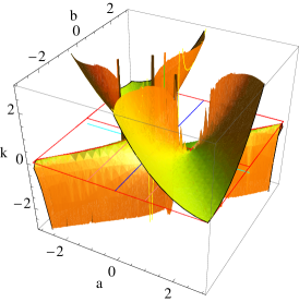
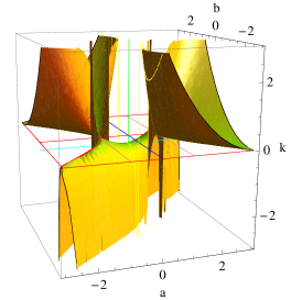
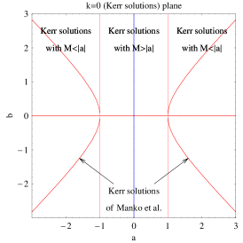
Figure 1: The first two plots show the parameter space $(a,b,k)$ of the two-soliton solution for a specific mass ($M=1$) from two different view points. The 2D surface plotted is the constrain of $k$ which corresponds to the Manko et al. solution [5, 7] used by Berti and Stergioulas [12]. The third plot is the $k=0$ plane of the parameter space which corresponds to all Kerr solutions of the two-soliton solution. The plots clearly show that the Manko et al. solution has no set of parameters that describe the case of $k=0$ which corresponds to the Kerr and the Schwarzschild (for $a=0$) solutions, since there is no intersection between the constrain of $k$ and the Kerr plane within the appropriate range of parameters. The two hyperbola plotted on the plane $k=0$ are the points were the constrain of $k$ touches the plane in a tangent manner. As we can see these hyperbola correspond to $|a|>M$.

As we have mentioned earlier, the Manko et al. solution [5, 7] is obtained if we impose the constrain $M^{2}-a^{2}-b^{2}+2k-2d=0$ to the parameters. This is analogous to having a two dimensional surface in the parameter space. There are two things that could be pointed out about that surface, which is drawn in Fig. 1. The first is that the axis of $b$ (the blue line) that corresponds to the Schwarzschild solution doesn’t cross the surface and the second is that the Kerr solutions with $M>|a|$, that lie in the parameter space on the plane $k=0$ between the two red lines parallel to the $b$ axis, do not intersect the surface either.

Thus, this solution can reduce to Schwarzschild or Kerr only formally. These are important drawbacks and were pointed out by Berti and Stergioulas [12]. Particularly important is the fact that it can only be matched with rapidly rotating models of neutron stars, since in the limit of zero rotation it has a non-vanishing quadrupole moment $Q=-\frac{M}{4}\frac{(M^{2}+b^{2})^{2}}{(M^{2}-b^{2})}$. These problems do not exist for the two-soliton solution, that can represent neutron stars of arbitrary rotation. Another important aspect of the two-soliton is that, as can be seen from the multipole moments (2), the solution can describe spacetimes with an arbitrary quadrupole $M_{2}$ and an arbitrary current octupole $J_{3}$, since every parameter is introduced linearly in the first moment it appears and thus it can always be determined by the first four non-zero moments.

3 Matching and comparison of the analytical to the numerical metric.

3.1 Matching of the analytical to the numerical solution.

In matching the analytical solution to the numerical one it is desirable to find a criterion that will be characteristic of the whole structure of the spacetime and not of a small region of it. That is, the matching conditions should be global and not local. Berti and Stergioulas [12] have argued that these global conditions should be the matching of the multipole moments. We will work under the same assumption. The multipole moments of a stationary axially symmetric spacetime are connected to the Ernst potential on the axis of symmetry and the spectrum of the moments fully specify it. On the other hand, when the Ernst potential on the axis is given, there exists a spacetime which is fully specified by that Ernst potential [14]. Thus, the multipole moments are characteristic of a spacetime and can be used as a global matching condition.

When a numerical spacetime for a neutron star model is constructed from a numerical algorithm, it is possible to evaluate its mass moments $M,\,Q,...$ and angular momentum moments $J,\,S_{3},...$ (for further discussion see Berti and Stergioulas [12]). These numerically evaluated moments can be used to impose the matching conditions to the analytical spacetime. The first four nonzero multipole moments of the two-soliton solution are:

$$M_{0}=M J_{1}=aM,$$ ,

$$M_{2}=-(a^{2}-k)M J_{3}=-(a^{3}-(2a-b)k)M,$$ , (9)

where we can see that once we specify the mass and the angular momentum of the spacetime, the parameter $k$ is uniquely determined by the quadrupole moment $Q=M_{2}$ and the parameter $b$ is uniquely determined by the current octupole $S_{3}=J_{3}$. Thus, having specified the parameters of the two-soliton, we have completely determined the analytical spacetime that can be used to describe the exterior of the neutron star. What remains to be seen is how well do the properties of the analytical spacetime compare to those of the numerical one.

3.2 Criteria for the comparison of the analytical to the numerical spacetime.

To compare the analytical to the numerical spacetime, one should use criteria that are characteristic of the geometric structure of the spacetime. The criteria should also be related to properties of the spacetime that could potentially be measured in astrophysical phenomena. A good fit of such properties would mean that they could be used to identify a spacetime through observational data and then associate it with properties of the compact object that generates it.

The first and more obvious criterion one can use is how well the respective components of the analytical and the numerical metric match. If the relative difference of the analytical metric components

$$g_{tt}=-f,\quad g_{t\phi}=f\omega,\quad g_{\phi\phi}=f^{-1}\rho^{2}-f\omega^{2}$$ (10)

to the corresponding numerical is small, one could consider the former as a good substitute of the latter. The comparison of the $g_{\phi\phi}$ component can be performed through the circumferential radius $R_{circ}=\sqrt{g_{\phi\phi}}$ which is as an indicator of how well the measurements of the circumferences in the corresponding spaces (analytical and numerical) with a specific value of the coordinate $\rho$, compare with each other.

The second criterion is the innermost stable circular orbit (ISCO). Test particles that move on geodesics on the equator follow trajectories that are given by the equation

$$-g_{\rho\rho}\left(\frac{d\rho}{d\tau}\right)^{2}=1-\frac{\tilde{E}^{2}g_{\phi\phi}+2\tilde{E}\tilde{L}g_{t\phi}+\tilde{L}^{2}g_{tt}}{\rho^{2}}\equiv V(\rho)$$ (11)

where $\tilde{E}$ and $\tilde{L}$ are the conserved energy per unit mass and angular momentum (parallel to the axis component) per unit mass and $V(\rho)$ is the effective potential. Since we are interested in circular orbits, the conditions for such orbits are $d\rho/d\tau=0$ and $d^{2}\rho/d\tau^{2}=0$ which are equivalent from (11) to the conditions for the effective potential, $V(\rho)=0,\quad dV(\rho)/d\rho=0$. The ISCO is determined if we additionally impose the condition that the radius $\rho$ of the circular orbit is also a turning point of the potential, that is $d^{2}V(\rho)/d\rho^{2}=0$. The location of the ISCO is of astrophysical importance since it indicates the radius at which matter orbiting a compact object can no longer maintain its orbit and plunges into the object. That radius would be the internal radius of accretion disks formed around such a compact object.

The third criterion is the rotation frequency of circular orbits on the equatorial plane. The rotation frequency $\Omega\equiv\frac{d\phi}{dt}$ is determined from (11) and the conditions for circular orbits, $V(\rho)=0,\quad dV(\rho)/d\rho=0$, and is given by the equation

$$\Omega(\rho)=\frac{-g_{t\phi,\rho}+\sqrt{(g_{t\phi,\rho})^{2}-g_{tt,\rho}g_{\phi\phi,\rho}}}{g_{\phi\phi,\rho}}.$$ (12)

The final criterion are the epicyclic frequencies $\Omega_{\rho},\;\Omega_{z}$. These are the frequencies of precession of the periastron and the orbital plane of a perturbed circular orbit, respectively. They can be evaluated by perturbing the equations of motion around a circular orbit

$$-g_{\rho\rho}\left(\frac{d\rho}{d\tau}\right)^{2}-g_{zz}\left(\frac{dz}{d\tau}\right)^{2}=V(\rho,z)$$ (13)

where $V(\rho,z)$ is the effective potential defined in (11) maintaining its $z$ dependence. The final expressions for the epicyclic frequencies are

$$\Omega_{a} = \Omega-\left\{-\frac{g^{aa}}{2}\left[(g_{tt}+g_{t\phi}\Omega)^{2}\left(\frac{g_{\phi\phi}}{\rho^{2}}\right)_{,aa}\right.\right.$$ (14)

$$-2(g_{tt}+g_{t\phi}\Omega)(g_{t\phi}+g_{\phi\phi}\Omega)\left(\frac{g_{t\phi}}{\rho^{2}}\right)_{,aa}$$

$$\left.\left.(g_{t\phi}+g_{\phi\phi}\Omega)^{2}\left(\frac{g_{tt}}{\rho^{2}}\right)_{,aa}\right]\right\}^{1/2},$$

where $a$ is $\rho$ or $z$ and the expression is evaluated at $z=0$ and around circular orbits of $\rho=\rho_{0}$.

These criteria can be related to astrophysical phenomena and in particular, they can be related to properties and observables of accretion disks. One such observable is the quasi-periodic oscillations (QPOs) with modulations in the range of kHz that have been observed in the X-ray flux from accreting X-ray pulsars [15]. The association of QPOs with the above frequencies could be used to determine the properties of the central object from the values of the various frequencies. These properties such as mass, angular momentum and mass quadrupole, could also be used to gain insight on the structure of the central object. Thus, an analytical spacetime that fits well all these parameters could be practically considered equivalent to the numerical one and a useful tool for doing astrophysics.

3.3 Results of the comparison.

In the comparison of the metric components, we have used the two corresponding Manko et al. solutions that were used by Berti and Stergioulas [12], as a reference. The comparison of the metrics is performed on the equatorial plane and on the axis of rotation. Here we will present only one rotating neutron star model, since these results are typical for all models. The chosen example is the one in table 3 of the Berti and Stergioulas [12] work, that corresponds to the model with the fastest rotation of the sequence of maximum mass in the non-rotating limit, for the FPS equations of state (EOS).

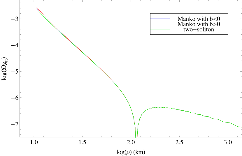
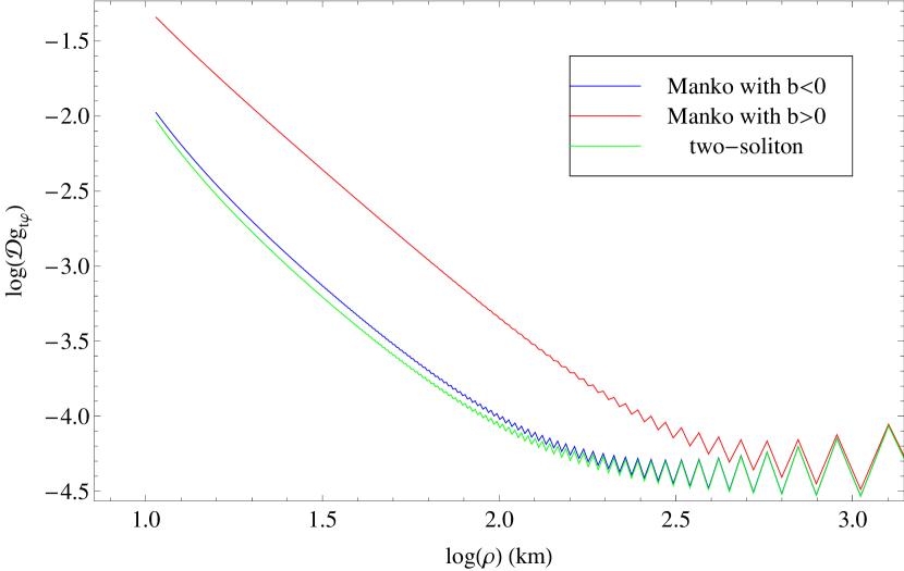
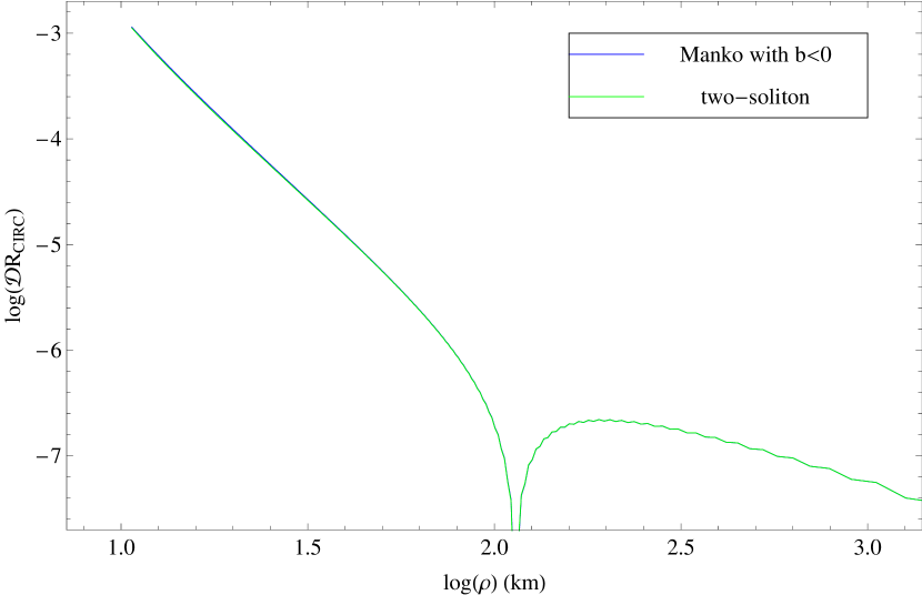
Figure 2: The first two plots show the relative difference of the three analytical metrics with the numerical for the components $g_{tt}$ and $g_{t\phi}$ on the equatorial plane. The analytical metrics used are the two-soliton and the two Manko et al. [5, 7] that correspond to the two values of the parameter $b$ (see Berti and Stergioulas [12]). The third plot shows the relative difference of the circumferential radius on the equatorial plane for the two-soliton and the Manko et al. with the negative value of $b$ (the two solutions almost coincide). As we can see, the errors are well under 1 percent (for the green line) on the surface and fall outwards. The oscillations that appear in the second plot are due to the behavior of the numerical solution.

In Fig. 2 we have plotted the relative difference of the metric components $g_{tt}$ and $g_{t\phi}$ and of the circumferential radius $R_{circ}$ as a function of coordinate radius $\rho$ on the equatorial plane (the $\mathcal{D}$ operator is defined as $\mathcal{D}=$(numerical - analytical)/numerical). In the first two graphs we have used for comparison the Two Soliton solution and the two corresponding solutions of Manko et al. which are distinguished by their value of the parameter $b$ of the Ernst potential. We remind here that the Ernst potential of the Manko et al. solution is given by the expression

$$e(z)=\frac{(z-M-ia)(z+ib)+d-\delta-ab}{(z+M-ia)(z+ib)+d-\delta-ab},$$ (15)

$$\delta=\frac{-M^{2}b^{2}}{M^{2}-(a-b)^{2}},\quad d=\frac{1}{4}\left(M^{2}-(a-b)^{2}\right)$$

where there are only three independent parameters $M,\;a,\;b$ and for a particular quadrupole moment of the numerical solution (with fixed $M,\;a$) there may be no corresponding value of $b$ or there may be two values. For these two values of $b$ we can calculate two metrics which are the ones shown in the graphs. As the second graph shows, the one of the two Manko et al. solutions does not fit well with the numerical metric and thus it describes it poorly [12]. On the other hand, the other solution (corresponding to the negative value of $b$) is as good as the two-soliton metric. Both metrics are better than 1 percent on the equator and the relative difference falls with increasing radial coordinate $\rho$. The relative difference shows a kink at about 100km which is an artifact due to a crossing of the numerical and the analytical solutions and has no further physical meaning. In the third graph of Fig. 2 we have used only the one of the Manko et al. metrics (the one with negative $b$) and the two-soliton. The relative difference for the $R_{circ}$ is under 0.1 percent on the surface and falls with increasing radial coordinate $\rho$.

In Fig. 3 we have plotted the relative difference of $g_{tt}$ on the axis of symmetry. The plot shows the same good behavior of the analytical metric on the axis as on the equatorial plane. The behavior on the axis of the analytical metric was a matter of confusion that has been clarified in [16].

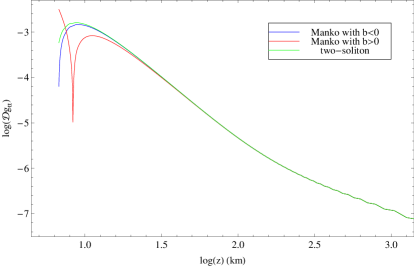
Figure 3: The plot shows the relative difference of the three analytical metrics with the numerical one for the component $g_{tt}$ on the axis of symmetry. The relative difference is under 1 percent on the surface. The behavior is similar to the behavior on the equatorial plane.

As we can see, both the Manko et al. and the two-soliton fit well the numerical metric. But for the Manko et al. there are constrains. If the rotation rate of the neutron star becomes smaller than a critical value (for typical values of the rotation parameter $j=J/M^{2}$ see [12]), there cannot be found any solutions (based on the first four multipole moments) of the type of Manko et al. that could match to the exterior of the neutron star. On the other hand, the two-soliton can describe arbitrary rotations as was pointed out and the good fit to the numerical metric extends to all rotations.

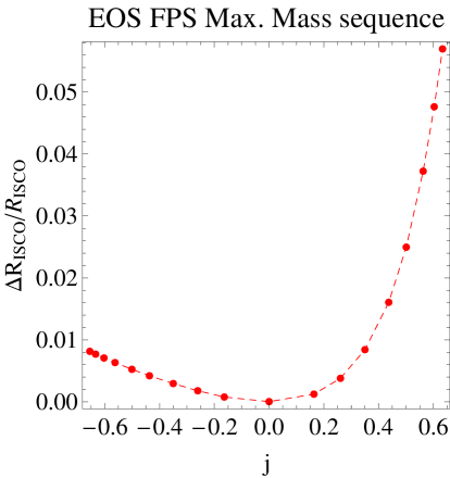
Figure 4: Relative difference of the analytical with the numerical ISCO for the sequence of maximum mass in the non-rotating limit for the equation of state FPS. The maximum difference of the co-rotating ISCO is 5.7 percent for the fastest rotating model that has a co-rotating ISCO and the maximum difference for the counter rotating ISCO is less than 1 percent for the fastest rotating model.

For the comparison of the ISCO we have used a sequence of models of neutron stars with various rotations. The sequence is the one in table 3 of Berti and Stergioulas [12] that corresponds to the model of maximum mass in the non-rotating limit for the FPS equation of state. The comparison of the $R_{ISCO}$ is shown in Fig. 4, where we have plotted the relative difference of the numerical ISCO with the analytical one as a function of the rotation parameter $j\equiv J/M^{2}$. The negative values of $j$ correspond to the counter-rotating ISCOs which are located further from the star surface. In some cases the co-rotating ISCO is under the surface of the star so, there is no numerical value for it, while that never happens for the counter-rotating ISCO. The co-rotating analytical ISCO is systematically less accurate than the counter-rotating one and that is to be expected since the latter is located further from the star. The difference in the ISCOs is less than 5.7 percent for the co-rotating and less than 1 percent for the counter-rotating orbits. The same general results are true for the Manko et al. metric for rotation parameters above the critical value. We should point out that the results of Fig. 4 are different than the ones shown in Fig. 8 of [12]. The difference is on the counter-rotating branch and it is due to a calculation slip that resulted to overestimation of the error in the counter-rotating ISCOs in [12]. For example the fastest rotating model of fig. 7 in [12] is given an error of 10 percent while the true error is of the order of 1.2 percent. Thus the ISCO comparison is more favorable than it was originally estimated.

The next property that we compare is the rotation frequency of the circular orbits. The relative difference of $\Omega$ on the equatorial plane is plotted as a function of the coordinate distance $\rho$ and is shown in Fig. 5. The relative difference is less than 1 percent on the surface of the star and reduces with increasing distance $\rho$. In this model, since the ISCO is located under the surface of the neutron star, there is no problem to evaluate $\Omega$ from the surface outwards. The analytically evaluated $\Omega$, as Fig. 5 shows, fits well the numerical $\Omega$ and that conclusion also holds for all rotations.

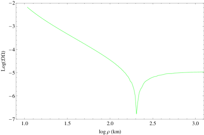
Figure 5: Relative difference in $\Omega$ of the two-soliton with the numerical metric. As in the plots of the various metric components, the relative difference is under 1 percent on the surface and falls outwards.

3.4 Conclusions

That was a brief presentation of our results on comparing the analytical two-soliton metric with numerical metrics describing the exterior of neutron stars. We plan to present a more thorough comparison between the two kinds of metrics in a forthcoming paper [17] where the comparison of the epicyclic frequencies will be demonstrated as well.

The results presented here suggest that the two-soliton metric is a very good candidate for describing the exterior spacetime of a neutron star of arbitrary rotation. Therefore, we could use this metric to gain information about the neutron star through observables related to astrophysical processes in the vicinity of the star.

I would like to thank Theocharis Apostolatos and Nikolaos Stergioulas for many useful discussions. This work was supported by the research funding program “Kapodistrias” with Grant No 70/4/7672.

References

References

- [1] Stergioulas N and Friedman J L 1995 ApJ 444 306.
- [2] Stergioulas N 2003 Rotating Stars in Relativity Living Rev. Relativity 6 3.
- [3] Ernst F J 1968 Phys. Rev. 167 1175, Ernst F J 1968, Phys. Rev. 168 1415.
- [4] Manko V S, Martin J and Ruiz J E 1995 J. Math. Phys. 36 3063.
- [5] Manko V S, Sanabria-Gómez J D and Manko O V 2000 Phys. Rev. D 62 044048.
- [6] Ruiz E, Manko V S and Martin J 1995 Phys. Rev. D 51 4192.
- [7] Manko V S, Mielke E W and Sanabria-Gómez J D 2000 Phys. Rev. D 61 081501.
- [8] Sibgatullin N R 1984 Oscilations and Waves in Strong Gravitational and Electromagnetic Fields (Nauka, Moscow, 1984; English translation: Springer-Verlag, Berlin, 1991).
- [9] Manko V S and Sibgatullin N R 1993 Class. Quantum Grav. 10 1383.
- [10] Papapetrou A 1953 Ann.Phys. 12 309.
- [11] Sotiriou T P and Pappas G 2005 J. Phys.: Conf. Ser. 8 23 (Preprint gr-qc/0504122).
- [12] Berti E and Stergioulas N 2004 MNRAS , 350 1416.
- [13] Stute M and Camenzind M 2002 MNRAS 336 831.
- [14] Hoenselaers C, Kinnersley W and Xanthopoulos B C 1979 Phys. Rev. Lett. 42 481, Hoenselaers C, Kinnersley W and Xanthopoulos B C 1979 J. Math. Phys. 20 2530, Xanthopoulos B C 1979 J. Phys. A: Math. Gen. 12 1025, Xanthopoulos B C 1981 J. Math. Phys. 22 1254, Hauser I and Ernst F J 1981 J. Math. Phys. 22 1051.
- [15] Kluzniak W, Abramowicz M A, Kato S, Lee W H and Stergioulas N 2004 Astrophys. J. 603 L89 (Preprint astro-ph/0308035).
- [16] Pappas G and Apostolatos T A 2008 Class. Quant. Grav. 25 228002 (Preprint 0803.0602 [gr-qc]).
- [17] Pappas G and Apostolatos T A, Work in preperation.