Spontaneous formation of synchronization clusters in homogenous neuronal ensembles induced by noise and interaction delays

Abstract

Spontaneous formation of clusters of synchronized spiking in a structureless ensemble of equal stochastically perturbed excitable neurons with delayed coupling is demonstrated for the first time. The effect is a consequence of a subtle interplay between interaction delays, noise and the excitable character of a single neuron. Dependence of the cluster properties on the time-lag, noise intensity and the synaptic strength is investigated.

Collective behavior in large ensembles of physiological and inorganic systems can be reduced to that of coupled oscillators engaged in various synchronization phenomena. In terms of macroscopic coherent rhythms, it may either be the case where all the units are recruited into a giant component or the case of cluster states characterized by exact or in-phase intra-subset and lag inter-subset synchronization. The spontaneous onset of cluster states is of particular interest to neuroscience clusters for the conjectured role in information encoding, as well as for participating in motor coordination or accompanying some neurological disorders. The approach to clustering has mostly relied on modeling neurons as autonomous oscillators, treating separately the question of whether the proposed mechanisms may be robust under noise us1 and transmission delays PitovskyN . We explore a new mechanism which rests on the excitable character of neuronal dynamics and mutual adjustment between noise and time delay to yield the self-organization into functional modules within an otherwise unstructured network.

For the instantaneous couplings, the research on populations of excitable neurons has covered pattern formation due to local inhomogeneity FHN1 , or has invoked a scenario where noise enacts a control parameter tuning the dynamics of ensemble averages between the three generic global regimes FHN2 . Distinct from the layout with complex connection topologies, here it is demonstrated how coupling delays do alter the latter landscape in a significant fashion, giving rise to an effect one may dub the cluster forming time-delay-induced coherence resonance. In part, the strategy to analyze global dynamics rests on deriving the mean-field (MF) approximation for the exact system. The likely gain from the MF treatment is at least twofold: except for allowing one to extrapolate what occurs in the thermodynamic limit $N\rightarrow\infty$, it may serve as an auxiliary means to discriminate between the effects of noise and time delay. Unexpectedly, the MF model undergoes a global bifurcation at certain parameter values where the exact system shows an onset of cluster states.

Network dynamics and the tools to analyze it– We focus on an $N$-size population of all-to-all diffusively coupled Fitzhugh-Nagumo neurons, whose local dynamics is set by

$$\epsilon dx_{i} =(x_{i}-x_{i}^{3}/3-y+I)dt+\frac{c}{N}\sum_{j=1}^{N}[x_{j}(t-\tau)-x_{i}(t)]dt,$$

$$dy_{i} =(x+b)dt+\sqrt{2D}dW_{i},$$ (1)

where the activator variables $x_{i}$ embody the membrane potentials, while the recovery variables $y_{i}$ mimic the action of the $K^{+}$ membrane gating channels. $c$ denotes the synaptic strength and $\tau$ stands for the coupling delay, both parameters for simplicity assumed homogeneous across the ensemble. The $\sqrt{2D}dW_{i}$ terms represent stochastic increments of the independent Wiener processes, i.e. the white noise. For the external stimulation holds $I=0$, whereas the small parameter $\epsilon=0.01$ warrants a clear separation between the fast and slow time scales. Selecting $b=1.05$, the neurons are poised near the Hopf bifurcation threshold $b=1$, which places them in an excitable regime where each possesses a single equilibrium. An adequate stimulation, be it by the noise or the interaction term, may evoke a large excursion of membrane potential, passing through the spiking and refractory states before it loops back to rest.

To characterize the degree of correlation between the firing events, we use primarily the interneuron spike train coherence coherence $\kappa_{ij}={\sum_{k=1}^{m}X_{i}(k)X_{j}(k)}/{\sqrt{\sum_{k=1}^{m}X_{i}(k)X_{j}(k)}}.$ This requires one to split the simulation period $T$ into bins $k$ of length $\Delta=T/m$, awarding each neuron a variable $X_{i}(k)=1(0)$, contingent on whether a spike was triggered or not within the given time bin, respectively. As with all the quantities below, we have been careful to exclude from calculations the transient behavior. The spike threshold and the time bin are set to $X_{0}=1$ and $\Delta=0.008$, verifying that no change of the results occurred if $X_{0}$ or $\Delta$ were reduced. The distribution of the $\kappa_{ij}$ values may serve to distinguish between the homogeneous and clustered network states. Another aspect we are interested in is whether the clustered states are monostable or coexistent with the homogeneous ones at the given network size. To probe this, we have monitored if the values of the global coherence $\kappa=\frac{1}{N(N-1)}\sum\limits_{i,j=1;i\neq j}^{N}\kappa_{ij}$ for different realizations at the fixed parameters clumped together, expecting bunching into distinct groups as evidence of multistable behavior.

Addressing the temporal structure of the network states, it is useful to look into the distribution of the local neuron jitters $r_{i}$ jitter . They represent the normalized variations of the interspike intervals $T_{k}$ extracted from $x_{i}(t)$, $r_{i}=\sqrt{<T_{k}^{2}>-<T_{k}>^{2}}/<T_{k}>$, with smaller values indicating better regularity. The modality and the width of the $r_{i}$ distribution over the population may serve as rough indices on how the cluster dynamics is mutually adjusted. In the final part, we analyze the behavior of the ensemble averages $X=1/N\sum_{i=1}^{N}x_{i}$ and $Y=1/N\sum_{i=1}^{N}y_{i}$, where the former increases if a larger fraction of neurons fire in synchrony. The results for the exact system are compared to those of the approximate MF model us4 . The latter presents a two-dimensional set of delayed differential equations

$$\epsilon\frac{dX(t)}{dt} =X(t)-X(t)^{3}/3-$$

$$-\frac{X(t)}{2}\left\{1-c-X(t)^{2}+\sqrt{[c-1+X(t)^{2}]^{2}+4D}\right\}$$

$$-Y(t)+c[X(t-\tau)-X(t)],$$

$$\frac{dY(t)}{dt} =X(t)+b,$$ (2)

derived within a cumulant approach by employing the Gaussian approximation.

We note that the results for the exact system refer to a network of $N=200$ neurons, applying independently a method from MG00 to verify no qualitative changes in the clustering behavior for larger $N$.

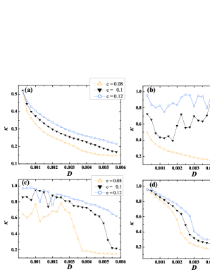
Figure 1: (color online). Profiles of the $\kappa(D)$ families of curves over the synaptic strengths $c=0.08,0.1$ and $0.12$ display strong dependence on the delay, increasing from $\tau=2$ in (a), $\tau=6$ in (b), $\tau=10$ in (c) to $\tau=11$ in (d). The location of ”wells” may point to the emergence of the clustered states.

Results– To get a sense of what may be the parameter ranges to admit the cluster states, we plot the $c$–families of the $\kappa$ curves in dependence of $D$ for different $\tau$. Without the delay, the curves would conform to a stereotype profile, where one distinguishes between the three ”regular” segments for very small, intermediate and large $D$, showing first a reduced $\kappa$ due to incoherent oscillations, then steady high values for the coherent ones and the decaying segment at $D$ where the stochastic dynamics prevails. However, from Fig. 1 we learn how this is upheld for some $\tau$, say $\tau=11$, but is violated manifestly at the ”cluster-resonant” values $\tau=2,6,10$. The ”wells” seen at approximately $D\in(0.001,0.003)$ in Figs. 1(b) and 1(c) may occur for just two reasons, as $\kappa$ decreases either for the incoherent or the clustered states. The latter alternative is supported by the coherence matrices in Fig. 3, which are discussed shortly. The importance of the $D$ - $\tau$ adjustment for the clustering effect is also witnessed by the $c$-dependence within the families in Fig. 1: the stronger the interaction term, the more salient is the picture of ”irregularity” sections immersed into a ”regular” curve profile. Increasing the delay, the cluster states first occur, apparently monostable, around $\tau=2$ for the small $D=0.00025$, whereby the typical phase portrait (PP) projection shows twisted orbits with two clearly discernable segments, see Fig. 2(a). These reflect the two macroscopic fractions of the population firing alternately, such that the homogeneous network dynamically splits into clusters of mutually synchronized neurons, with the clusters locked in antiphase. The frequency entrainment is indicated by the shape of the $r_{i}$ distribution, which peaks sharply around $<r>_{m}=0.01$. We tested the invariance of clustering with $N$ via the asymptotical behavior of the quantity $\chi^{2}_{N}=\frac{\sigma_{X}^{2}}{\frac{1}{N}\sum_{i=1}^{N}\sigma_{x_{i}}^{2}}$, where $\sigma_{X}^{2}=<X(t)^{2}>_{t}-<X(t)>_{t}^{2}$ and $\sigma_{x_{i}}^{2}=<x_{i}(t)^{2}>_{t}-<x_{i}(t)>_{t}^{2}$ holds. If the cluster states endure, there should be a residual component $\chi(\infty)\in(0,1)$ in the large $N$ limit MG00 . For this and the remaining cases, the onset of such a regime is found around $N\approx 200$, implying that no qualitatively novel phenomena occur above this system size. An interesting observation is that the cluster configuration $\left\{N_{1},N_{2}\right\}$, determined by the fractions’ sizes, fluctuates around the ratio $2:1$ for different stochastic realizations and appears to aggregate with enhancing $N$. For certain $\tau$, the $2$-cluster state also emerges outside the $D$-region delimiting the incoherent and coherent global regimes. This holds for $\tau=5$ and $D\in(0.0004,0.0008)$, where the cluster layout is also such that if one is active, the other remains refractory. The $r_{i}$ distribution maintains a narrow form, but its maximum shifts to $<r>_{m}\approx 0.19$. Though one retrieves the general picture from above, a variance is that larger $\tau$ seems to favor the partition $N_{1}/N_{2}\approx 1:1$, see PP in Fig. 2(b). The $1:1$ ratio is preferred both for increasing $N$ and if the delay is set to $\tau=6$.

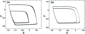
Figure 2: Global PPs for the $2$-cluster states show twisted LCs, whereby the two discernable segments reflect the alternate firing of the neuron subsets. The $N_{1}/N_{2}$ ratio depends on the interplay of $D$ and $\tau$, as seen from the examples $\tau=2,D=0.00025,c=0.1$ in (a) and $\tau=5,D=0.0005,c=0.1$ in (b).

The clustered states so far may be cast as stationary in the sense of stability against neurons switching between the clusters. We also report on the existence of $3$-cluster states that may be considered ”dynamical”, with the neurons able to jump to and from clusters. Such an outcome arises for the stronger noise $D\approx 0.0013$, once the delay is increased to $\tau=10$. To underline the difference between the stationary and dynamical clustered states at $\tau=5$ and $\tau=10$, we plot side-by-side the corresponding pairwise coherence matrices $\left\{\kappa_{ij}\right\}$, see Figs. 3(a) and 3(b), where the network nodes have been rearranged by a hierarchical clustering algorithm according to a form of metric distance that has the most coherent nodes the closest. This makes it explicit how the intercluster coherence for the $2$-cluster state is virtually negligible with respect to the $3$-cluster case. Loosely speaking, within an unstable three-part population division, when a certain fraction is firing, the other is refractory and the neurons in the smallest cluster are at rest (excitable). This less clear separation is also apparent when comparing the nodal degree distributions in cases $\tau=5$ and $\tau=10$, obtained if one assumes $\left\{\kappa_{ij}\right\}$ to provide weights for the network whose links stand for the correlated dynamics between the neurons. For $\tau=5$, the bimodal degree distribution is clearly seen without raising the connectivity threshold, whereas for $\tau=10$ the initially smeared three-modal distribution refines after some thresholding is performed. The rationale of dynamical clustering may best be understood by analyzing the $r_{i}$ distribution in the $3$-cluster state. Apart from being wider than in the $2$-cluster state, it peaks at a much smaller value $<r>_{m}\approx 0.09$, implying the more regular neuron firing. For this to hold, synchrony within the clusters has to be of intermittent nature, such that the neurons once engaged in synchronized spiking are much more likely to do so again.

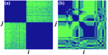
Figure 3: (color online). Rearranged coherence matrices for $\tau=5,D=0.0005,c=0.1$ in (a) and $\tau=10,D=0.0013,c=0.1$ in (b) imply the strong cluster separation in the $2$-cluster states and mixing between the clusters in the $3$-cluster case. Darker shading reflects higher coherence.

Aa understanding of clustering mechanism is revealed by comparing the typical PPs of neurons participant in the homogeneous coherent state and the clustered states, see Figs. 4(a) and 4(b). A striking feature in the latter case is a kink at the refractory branch of the slow manifold. The appearance of a kink is the key manifestation of the $D-\tau$ co-effect, that consists in separating the ensemble into clusters and maintaining the proper phase difference between them. The purpose of the kink is to keep the neurons frustrated long enough at the refractory branch before being allowed to slide down to its left knee. This may be imagined as a form of a lock-and-release behavior, where the delay primarily gives rise to the first, and noise to the second part. If a fraction of the ensemble were to move beyond the left knee and the other were to lag behind, the split should be amplified with each population cycle, eventually becoming resilient to perturbation precisely due to trapping at the refractory branch. For trapping to be successful, the kink has to be placed properly, approximately where the dynamics of the representative point is most susceptible to perturbation along the slow manifold. Then, for a brief period, due to an influence from $x_{i}$, the evolution of $y_{i}$ is locally accelerated, becoming comparable to a speed of change in the direction orthogonal to the slow manifold, driven by the spiking fraction of the population. Note that the trapping interval has to be adjusted so that the entire population is entrained to a single frequency of firing. The latter matches the one in delay-free case, which warrants stability against perturbations. The arguments above and the numerical data seem to indicate how the delays where the coherence resonance is felt the strongest may be approximated by $\tau=T_{0}/2+n*T_{0}$, with $T_{0}$ being the period of coherent oscillations at $\tau=0$. Noise-wise, with increasing $\tau$, $D$ has to be adjusted to higher values to regulate the relaxation from the kink to the slow manifold while maintaining the entrainment to the proper frequency. In parallel, for stronger $D$, the representation cloud of the firing fraction tends to disperse more, requiring a sufficient $\tau$ for this effect to be averaged out.

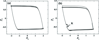
Figure 4: (a) and (b) show typical PPs of neurons participating the homogeneous global oscillations and clustered states, respectively. The latter are distinguished by a kink $K$, which is a signature of the $D-\tau$ co-effect. The parameter sets are $\tau=6,D=0.0005,c=0.1$ in (a) and $\tau=2,D=0.00025,c=0.1$ in (b).

The interplay between $D$ and $\tau$ is further highlighted by exploring the behavior of the MF model (2). Local bifurcation analysis shows that the MF exhibits a succession of super- and subthreshold Hopf bifurcations us4 , which account for the transition from the stochastically stable FP to the stable LC. Still, this scenario is confined to noise higher than here: analytical and numerical means corroborate the Hopf bifurcations to emerge about $D\approx 0.0025$ at relevant $\tau$. Now we argue that the approximate model is in qualitative terms able to capture the clustering effect occurring for small $D,c$ and $\tau$. Focus is on the finding that MF system predicts an onset of cluster states by undergoing a global bifurcation for the parameter values around $\tau=2,D=0.00025$ and $c=0.08$. At the given $\tau$ and $D$, for $c<0.08$ the approximate model has only the equilibrium, whereas around $c\simeq 0.08$ a large and a small LC are born via a fold-cycle scenario. Note how then the PP of the MF acquires the form qualitatively similar to those of the exact system’s in Figs. 2(a) and 2(b). The two sections of the emerging MF orbit mimic the action of the fractions within the full population. This structure of the LC becomes unstable under increasing $c$ or $\tau$, i.e. for the stronger impact of the interaction term. Another interesting aspect to the approximate system is that it shows the complex LC to coexist with the FP, viz. the basins of attraction in Fig. 5(b), which is a feature apparently absent in the exact model. However, the FP is located very close to the basins’ boundary which indicates it to be stochastically unstable in the exact system for an arbitrary small noise.

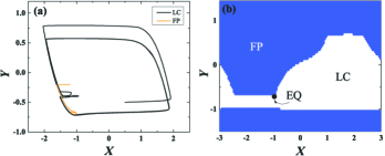
Figure 5: (color online). Bistability in the MF model: (a) shows the trajectories converging either to the FP or the LC, depending on the initial conditions, whereas in (b) are displayed the two basins of attraction for $\tau=2,D=0.00025,c=0.1$.

We have reported on a novel phenomenon where clustering within the homogeneous neural population is induced by an interplay of noise and time delay. This paradigm is distinct from most current explanations on how the clustered states may arise, for it does not treat $D$ and $\tau$ as destabilizing and detrimental, but rather as biased toward the formation of dynamical structure in networks that are unstructured both in terms of topology and local parameters. The analyzed model is minimal yet sufficient to display an interesting type of behavior, possible only as an interplay of excitability, noise and interaction delay. Once the phenomenon is recognized as caused only by these qualitative properties one can study the effects of more realistic assumptions on the distribution of neuronal properties and connection patterns. An interesting point concerns the derived MF model, which can aid in understanding the precise roles played by $D$ and $\tau$. Notably, beneath the surface lies a more stratified phenomenon, where the subtle adjustment between the parameters affects the number of clusters, their configuration, stationary or dynamical character, as well as whether the cluster states occur monostable or coexist with the homogenous solution at the given population size. This framework could find application within the research on neural systems and other excitable media.

- (1) P. A. Tass, Phase Resetting in Medicine and Biology: Stochastic Modelling and Data Analysis, (Springer, Berlin Heidelberg, 2007).
- (2) N. Burić and D. Todorović, Phys.Rev. E, 67, 066222 (2003); M. Dhamala, V. K. Jirsa and M. Ding, Phys. Rev. Lett, 92, 074104 (2004); S. H. Strogatz, Nature 394, 316 (1998); O. V. Popovych, C. Hauptmann and P. A. Tass, Phys. Rev. Lett. 94, 164102 (2005).
- (3) A. Pikovsky, A. Zaikin and M. A. de la Casa, Phys. Rev. Lett. 88 050601 (2002); B. Lindner, J. Garcia-Ojalvo, A. Neiman and L. Schimansky-Geier, Phys. Rep. 392, 321 (2004); N. Burić, K. Todorović and N. Vasović, Phys. Rev E, 75, 026209 (2007); Q. Wang, G. Chen and M. Perc, PLoS ONE 6, e15851 (2011).
- (4) X. Sailer et al., Phys. Rev. E 73, 056209 (2006).
- (5) P. Kalutza, C. Strege and H. Meyer-Ortmanns, Phys. Rev. E 82, 036104 (2010).
- (6) M. Yi and L. Yang, Phys. Rev. E 81, 061924 (2010); X. Sun, M. Perc, Q. Lu and J. Kurths, Chaos 20, 033116 (2010).
- (7) A. Pikovsky, J. Kurths, Phys. Rev. Lett. 78, 775 (1997); Y. Gao and J. Wang, Phys. Rev. E 83, 031909 (2011).
- (8) Neuro-Informatics and Neural Modelling, edited by F. Moss and S. Gielen (Elsevier, Amsterdam, 2000), p. 903.
- (9) N. Burić, K. Todorović and N. Vasović, Phys. Rev. E, 82, 037201 (2010)