How far can minimal models explain the solar cycle?

Abstract

A physically consistent model of magnetic field generation by convection in a rotating spherical shell with a minimum of parameters is applied to the Sun. Despite its unrealistic features the model exhibits a number of properties resembling those observed on the Sun. The model suggests that the large scale solar dynamo is dominated by a non-axisymmetric $m=1$ component of the magnetic field.

1. INTRODUCTION

During the past two decades the understanding of the process of magnetic field generation by motions of an electrically conducting fluid has progressed rapidly and increasingly realistic models of dynamos operating in planetary interiors have been achieved. Models of the geodynamo, of the ancient Martian dynamo or of Mercury’s dynamo are primarily restricted by the lack of knowledge of certain properties of the respective planetary core. The dynamo process operating in the Sun, on the other hand, is still subject to controversies with several competing proposals. The density variations of several orders of magnitude in the solar convection zone and the complications introduced by the compressibility of the fluid have prevented so far a fully convincing model of the solar cycle.

In this situation it can be helpful to consider the properties of a most simple physically consistent model of convection driven dynamos in a rotating spherical shell in order to see which properties might resemble those of the solar cycle. Assuming a given radius ratio of the spherical fluid shell the minimum number of dimensionless parameters is four, namely the Rayleigh number $R$, the rotation parameter $\tau$, the Prandtl number $P$ denoting the ratio of viscous and thermal diffusivity, and the magnetic Prandtl number $P_{m}$ denoting the ratio of viscous and magnetic diffusivity.

The success of numerical simulations of the generation of magnetic fields by turbulent fluid motions relies of the concept of eddy diffusivities which represent the diffusive actions of small scale turbulence that remains unresolved in the numerical schemes. The ratios of those eddy diffusivities are expressed by the values of $P$ and $P_{m}$ used in the numerical computations. Frequently the assumption $P=P_{m}=1$ is made based on the argument that the turbulent diffusion affects the transport of heat, momentum and magnetic flux in the same way. This assumption is not correct, however, since the transports of scalar and vector quantities are affected in different ways (Kays et al.,, 2005; Yousef et al.,, 2003). Moreover, the diffusivities in the absence of any motion often differ by many orders of magnitude, - in particular when the radiative transport is taken into account in the heat diffusivity -, such that even highly turbulent fluids do not fully erase differences in the effective diffusivities.

Even if it is assumed that ratios of the effective diffusivities for heat, momentum and magnetic flux do not differ much from unity in the highly turbulent solar convection zone, it must be realized that numerical simulations of convection driven dynamos depend sensitively on the parameters $P$ and $P_{m}$ near their values of unity. In particular it has been found that a transition between two different types of dynamos occurs which is hysteretic as a function of $P$ and $P_{m}$ (Simitev & Busse, 2009). It thus appears to be of interest to study simple convection driven dynamos in dependence on these two parameters in addition to the Rayleigh number and the rotation parameter. More realistic solar dynamo models involve many more parameters and because of the high demand for numerical resolution the opportunities for comprehensive studies of parameter dependences are restricted.

For the present study a numerical model for convection driven dynamos that previously has been employed for investigations motivated by problems of the geodynamo (see, for example, Simitev & Busse,, 2005) has been modified for solar applications. A much thinner spherical shell is assumed and no-slip conditions at the inner boundary and stress-free conditions at the outer boundary are used. The Boussinesq approximation has been retained even though it is not appropriate for any realistic solar dynamo model and causes an unrealistic dependence of the solar differential rotation on depth. Nevertheless, as we hope to demonstrate, there are properties of the dynamo solutions that resemble those observed on the Sun.

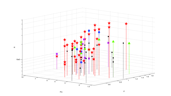
Figure 1.— (Color online) Convection-driven dynamos as a function of $R$, $P$ and $P_{m}$ for $\tau=2000$. Decaying dynamos are indicated by black dots, MD dynamos are indicated by blue diamonds, FD dynamos are indicated by red stars, quadrupolar dynamos are indicated by green triangles, and coexisting MD and FD dynamos are indicated by pink squares.

2. MATHEMATICAL FORMULATION

We consider a spherical fluid shell rotating about a fixed vertical axis. The basic equations permit a static solution with the temperature distribution

$$T_{S}=T_{0}+\Delta T\eta r^{-1}(1-\eta)^{-2},$$

where $r$ denotes the distance from the center of the spherical shell measured in multiples of the shell thickness $d$. The ratio of inner to outer radius of the shell is denoted by $\eta$. $\Delta T$ is thus the temperature difference between the two boundaries. The gravity field is given by ${\bf g}=-d\gamma{\bf r}.$ In addition to $d$, the time $d^{2}/\nu$, the temperature $\nu^{2}/\gamma\alpha d^{4}$, and the magnetic flux density $\nu(\mu\varrho)^{1/2}/d$ are used as scales for the dimensionless description of the problem where $\nu$ denotes the kinematic viscosity of the fluid, $\kappa$ its thermal diffusivity, $\varrho$ its density, and $\mu$ its magnetic permeability. The equations of motion for the velocity vector ${\bf u}$, the heat equation for the deviation $\Theta$ from the static temperature distribution, and the equation of induction for the magnetic flux density ${\bf B}$ are thus given by

$$\partial_{t}{\bf u}+{\bf u}\cdot\nabla{\bf u}+\tau{\bf k}\times{\bf u}=-\nabla\pi+\Theta{\bf r}+\nabla^{2}{\bf u}+{\bf B}\cdot\nabla{\bf B},$$ (1)

$$\nabla\cdot{\bf u}=0,$$ (2)

$$P(\partial_{t}\Theta+{\bf u}\cdot\nabla\Theta)=(R\,\eta r^{-3}(1-\eta)^{-2}){\bf r}\cdot{\bf u}+\nabla^{2}\Theta,$$ (3)

$$\nabla\cdot{\bf B}=0,$$ (4)

$$\nabla^{2}{\bf B}=P_{m}(\partial_{t}{\bf B}+{\bf u}\cdot\nabla{\bf B}-{\bf B}\cdot\nabla{\bf u}),$$ (5)

where $\partial_{t}$ denotes the partial derivative with respect to time $t$ and where all terms in the equation of motion that can be written as gradients have been combined into $\nabla\pi$. The Boussinesq approximation is assumed in that the density $\varrho$ is regarded as constant except in the gravity term where its temperature dependence, given by $\alpha\equiv-(\partial\varrho/\partial T)/\varrho=$const., is taken into account. The Rayleigh numbers $R$, the Coriolis number $\tau$, the Prandtl number $P$ and the magnetic Prandtl number $P_{m}$ are defined by

$$R=\frac{\alpha\gamma\Delta Td^{4}}{\nu\kappa},\enspace\tau=\frac{2\Omega d^{2}}{\nu},\enspace P=\frac{\nu}{\kappa},\enspace P_{m}=\frac{\nu}{\lambda},$$ (6)

where $\lambda$ is the magnetic diffusivity. Because the velocity field ${\bf u}$ as well as the magnetic flux density ${\bf B}$ are solenoidal vector fields, the general representation in terms of poloidal and toroidal components can be used

$${\bf u}=\nabla\times(\nabla v\times{\bf r})+\nabla w\times{\bf r}\enspace,$$ (7)

$${\bf B}=\nabla\times(\nabla h\times{\bf r})+\nabla g\times{\bf r}\enspace.$$ (8)

Equations for $v$ and $w$ are obtained by multiplication of the curl² and of the curl of equation (1) by ${\bf r}$. Analogously equations for $h$ and $g$ are obtained through the multiplication of equation (5) and of its curl by ${\bf r}$.

No-slip boundary conditions will be used at the inner boundary and stress-free conditions are applied at the outer boundary, while the temperature is assumed to be fixed at both boundaries,

$$v=\partial_{r}v=w=\Theta=0\quad\mbox{ at }r=r_{i}\equiv\eta/(1-\eta)$$ (9)

$$v=\partial^{2}_{rr}v=\partial_{r}(w/r)=\Theta=0\quad\mbox{ at }r=r_{o}\equiv 1/(1-\eta).$$ (10)

For the magnetic field, electrically insulating boundaries are assumed such that the poloidal function $h$ must be matched to the function $h^{(e)}$, which describes the potential fields outside the fluid shell

$$g=h-h^{(e)}=\partial_{r}(h-h^{(e)})=0\quad\mbox{ at }r=r_{i}\mbox{ and at}\quad r=r_{o}.$$ (11)

Throughout this paper we shall use $\eta=0.65$.

The numerical integration proceeds with a pseudo-spectral method as described by Tilgner (1999) which is based on an expansion of all dependent variables in spherical harmonics for the $\theta,\varphi$-dependences, i.e.

$$v=\sum\limits_{l,m}V_{l}^{m}(r,t)\,P_{l}^{m}(\cos\theta)\,\exp(im\varphi)$$ (12)

and analogous expressions for $w,\Theta,h$ and $g$. Here $P_{l}^{m}$ denotes the associated Legendre functions. For the $r$-dependence expansions in Chebychev polynomials are used. For the computations to be reported in the following a minimum of 41 collocation points in the radial direction and spherical harmonics up to the order 128 have been used.

The numerical model outlined above is essentially the same as has been used by Gilman & Miller (1981) and Gilman (1983). At that time, 30 years ago, computer resources allowed time integrations only for a few selected parameter values and the phenomenon of bistability (see below) was not yet known. It thus seems appropriate to return to the most simple physically consistent formulation of convection driven dynamos in rotating spherical fluid shells as formulated in this section.

3. DYNAMO SOLUTIONS IN DEPENDENCE ON $P$ AND $P_{m}$

In choosing parameter values in our model we follow Gilman (1983) in selecting a value around $2000$ for $\tau$ which in the case of the Sun corresponds to an eddy viscosity $\nu=1.6\times 10^{8}$ m²/s. Values for $R$ have usually been selected within a range of up three times the value needed for dynamo action. Otherwise the dynamos become too chaotic and regular features disappear. Our study has thus focussed on the variations of dynamos with the parameters $P$ and $P_{m}$.

In figure 1 the existence of solutions for convection driven dynamos in the $(P,P_{m},R)$–space is outlined. In order to achieve dynamo action the Rayleigh number $R$ must be sufficiently high such that the magnetic Reynolds number $R_{m}$ exceeds a critical value. The latter is inversely proportional to the magnetic Prandtl number $P_{m}$. Since our study focusses on reasonably regular dynamos we have found it difficult to obtain dynamos for small values of $P_{m}$ since dynamos will become highly chaotic in this case or even decay. As indicated in figure 1 there exist a large variety of dynamos ranging from dipolar to quadrupolar ones. At higher Rayleigh numbers the dynamos are often of mixed polarity. While most of the dynamo solutions have been obtained for the radius ratio $\eta=0.65$, some cases obtained for $\eta=0.6$ have been added in the figure since it was found that the dynamos depend only weakly on this parameter.

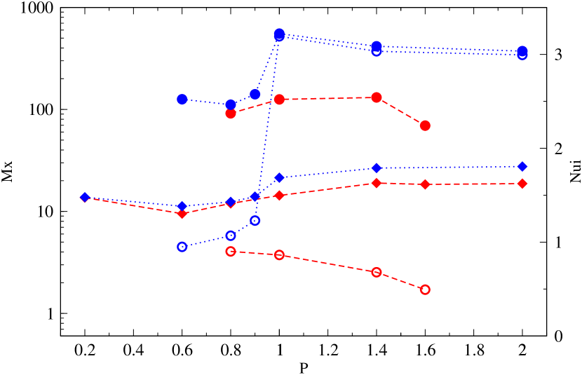
Figure 2.— (Color online) Coexisting nonlinear dynamo solutions at identical parameter values in the case $\eta=0.65$ $\tau=2000$, $R=150000$ and $P/P_{m}=0.2$. The fluctuating poloidal magnetic energy component $\check{M}_{p}$ (solid circles) and the mean poloidal magnetic energy component $\overline{M}_{p}$ (empty circles) are scaled on the left ordinate, while the Nusselt number at $r=r_{i}$ (solid diamonds) is scaled on the right ordinate. Cases started from initial conditions on the FD branch are shown in red and connected by dashed lines, and those started from initial conditions on the MD branch are shown in blue and connected by dotted lines.

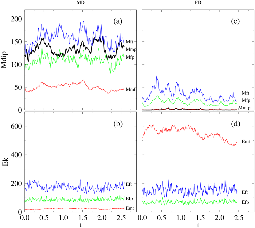
Figure 3.— (Color online) Coexisting distinct nonlinear dynamo solutions at identical parameter values – a MD (left column (a,b)) and a FD dynamo (right column (c,d)) both at $R=1.5\times 10^{6}$, $\tau=2\times 10^{4}$, $P=1$ and $P_{m}=5$. Panels (a,c) and (b,d) show time series of magnetic dipolar energy densities and kinetic energy densities, respectively. The component $\overline{X}_{p}$ is shown by thick solid black line, while $\overline{X}_{t}$, $\check{X}_{p}$, and $\check{X}_{t}$ are shown by red, green and blue lines, respectively, and labeled. $X$ stands for either $M$ or $E$.

Of particular interest is the distinction between MD-dynamos which are dominated by a strong and nearly steady axisymmetric dipolar magnetic field and the FD-dynamos for which magnetic energies of the axisymmetric components are far less than those of the non-axisymmetric components and which exhibit a cyclic behavior. Over a considerable extent of the parameter range these two types of dynamos exist simultaneously at the same values of the external parameters as demonstrated by the example of figure 2. It is remarkable that the two types of dynamos exhibit nearly the same Nusselt number. This property indicates that both types are similarly efficient in the use of the available buoyancy. For more details on the phenomenon of bistability we refer to the paper by Simitev & Busse (2009). A comparison of the magnetic and kinetic energy densities for the two types of dynamos is shown in figure 3. Here the definitions

$$\bar{M}_{p}=\langle\mid\nabla\times(\nabla\bar{h}\times{\bf r})\mid^{2}\rangle/2,\quad \bar{M}_{t}=\langle\mid\nabla\bar{g}\times{\bf r}\mid^{2}\rangle/2$$ (13)

$$\check{M}_{p}=\langle\mid\nabla\times(\nabla\check{h}\times{\bf r})\mid^{2}\rangle/2,\quad \check{M}_{t}=\langle\mid\nabla\check{g}\times{\bf r}\mid^{2}\rangle/2$$ (14)

have been used where the angular brackets indicate the average over the fluid shell and where $\bar{h}$ refers to the azimuthally averaged component of $h$ and $\check{h}$ is given by $\check{h}=h-\bar{h}$. Analogous relationships hold for the kinetic energy densities for which $M,h,g$ are replaced by $E,v,w$.

Near the end points of the bistability regions transitions from MD- to FD-dynamos and vice versa may, of course, occur owing to exceptionally large fluctuations. Such a transition was observed in the long-time dynamo integration of Goudard & Dormy (2008). As their convection driven dynamo changed from the MD-state to the FD-state these authors noted a solar like behavior in butterfly-like diagrams in which they had plotted the axisymmetric $\varphi$-component of the magnetic field, $\overline{B}_{\varphi}$, as a function of latitude and time. As must be expected from the decrease with depth of their differential rotation (Yoshimura,, 1975), the waves of the butterfly diagram propagated to higher latitudes instead of lower ones. It turns out, however, that non-axisymmetric components of the azimuthal magnetic field are comparable in amplitude to the axisymmetric component $\overline{B}_{\varphi}$. It thus appears to be appropriate to study these dynamos in more detail.

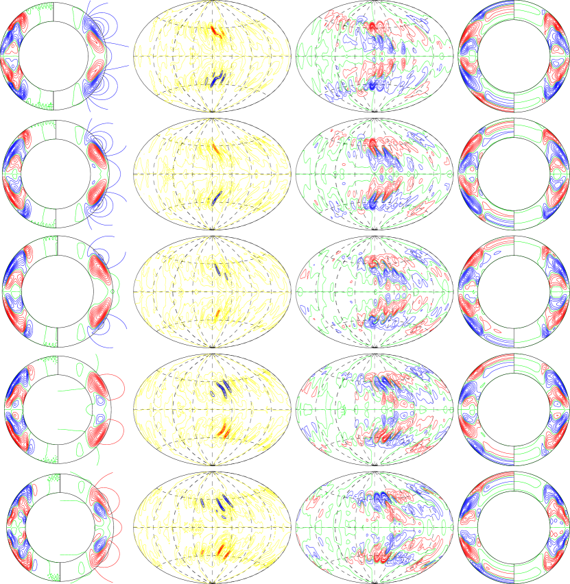
Figure 4.— (Color online) Approximately half a period of a dynamo oscillation in the case $\tau=2000$, $R=120000$, $P=1.2$, $P_{m}=4.5$. The first column shows meridional lines of constant $\overline{B_{\varphi}}$ on the left and poloidal fieldlines, $r\sin\theta\partial\overline{h}/\partial\theta$ on the right. The second column shows lines of constant horizontal magnetic field $(B_{\varphi}^{2}+B_{\theta}^{2})^{1/2}$ at $r=0.9$ corresponding to $-0.9$, $-0.8$, $-0.7$, $0.7$, $0.8$, $0.9$ of its maximum absolute value with the sign determined by the sign of $B_{\varphi}$, and the third column shows lines of constant $B_{r}$ at $r=r_{o}$. The last column shows $\mathrm{Re}(\partial g^{m=1}/\partial\theta)$ to the left and $\mathrm{Im}(\partial g^{m=1}/\partial\theta)$ to the right. The five rows are separated equidistantly in time by $\Delta t=0.0224$.

In figure 4 a typical example of a nearly periodic FD-dynamo is shown. In the four columns of plots the development of various components of the magnetic field is shown in five equidistant steps in time covering about half a period of the magnetic cycle. As is evident from the radial component $B_{r}$ displayed in the third column, the dynamo appears to operate mainly in one of two meridional hemispheres. In the second column maxima of the horizontal magnetic field at the depth of 0.1 from the surface have been indicated as a measure of the likelihood of the appearance of sunspots. Since the underlying hemispherical structure hardly moves the pattern of the second column seems to reflect the phenomenon of the active longitude of sunspots see, for example, Usoskin et al., (2007) and references therein or of solar X-ray flares (Zhang et al.,, 2007). Since sometimes the $m=2$-component of the magnetic field dominates instead of the $m=1$-component the phenomenon of two active longitudes 180 degrees apart can also be observed in the dynamo simulations. Persistent active longitudes have been detected in various types of active stars as well (Usoskin et al.,, 2007).

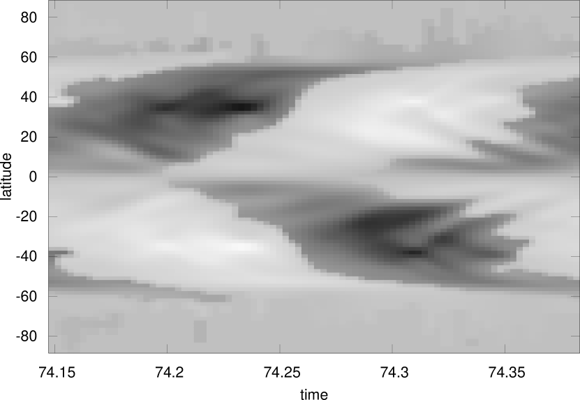
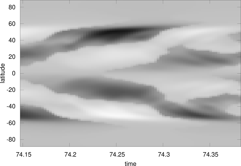
Figure 5.— ”Butterfly” diagrams: $B_{\varphi}^{m=0}+|B_{\varphi}^{m=1}|\mathrm{sgn}(B_{\varphi}^{m=0})$ (top) and $B_{r}^{m=0}+|B_{r}^{m=1}|\mathrm{sgn}(B_{r}^{m=0})$ (bottom) are plotted as functions of latitude and time in the case $P=1.2$, $\tau=2000$, $R=120000$, $P_{m}=4.5$.

In figure 5 two ”butterfly” diagrams have been plotted. Because the strength of the axisymmetric component of $B_{\varphi}$ alone is not representative of the horizontal magnetic field that may give rise to sunspots we have added in the upper plot the main non-axisymmetric component characterized by the azimuthal wavenumber $m=1$. While there is some wave-like movement towards lower latitudes, the main pattern moves towards high latitudes. This must be expected since the differential rotation decreases with depth Yoshimura, (1975). The movement toward higher latitudes is even more pronounced in the pattern of the radial component $B_{r}$ of the magnetic field as shown in the lower plot of figure 5. A phase shift between the patterns of the upper and the lower plot can also be noticed in that the sign change of $B_{r}$ occurs after that of $B_{\varphi}$. This feature agrees with the well known solar phenomenon that the change in the sign of $B_{r}$ occurs near the maximum of the sunspot cycle.

4. CONCLUSION

Most models of the solar cycle are based on essentially axisymmetric dynamos, but there are exceptions such as the dynamo proposed by Ruzmaikin et al., (1988) based on a mean field approach. It is not quite clear how strong the non-axisymmetric components of the solar toroidal magnetic field with wavenumbers $m=1$ or $m=2$ are in relation to the axisymmetric component. Estimates range from $0.1$ based on sunspot numbers (Usoskin et al.,, 2007) to $0.43$ based on powerful X-ray flares (Zhang et al.,, 2007). A main conclusion to be derived from the dynamo model outlined in this paper is that the large scale non-axisymmetric components are likely to be an important ingredient of solar magnetism. The well documented existence of active longitudes certainly supports this conclusion.

There are, of course, also major differences between solar phenomena and certain features of the present Boussinesq model. Some of these are well understood as for example the difference in the propagation of dynamo waves. This is most probably caused by the fact that the model always exhibits a differential rotation decreasing with depth for FD-type dynamos, while the Sun possesses a differential rotation that increases with depth in the uppermost $15\%$ of the convection zone. For a preliminary attempt to take this effect into account we refer to a recent companion paper by Simitev & Busse (2012).

References

- Gilman (1983) Gilman, P. A., 1983, Astrophys. J. Suppl., 53, 243
- Gilman & Miller (1981) Gilman, P. A., And Miller, J., 1981, Astrophys. J. Suppl., 45, 351.
- Goudard & Dormy (2008) Goudard, L., & Dormy, E. 2008, Europ. Phys. Letts., 83, 59001
- Kays et al., (2005) Kays, W., Crawford, M., and Weigand, B., Convective Heat and Mass Transfer, 2005 (McGraw-Hill, 4th edn)
- Ruzmaikin et al., (1988) Ruzmaikin, A.A., Sokoloff, D.D., & Starchenko, S.V., 1988, Solar Physics, 115, 5-15
- Simitev & Busse, (2005) Simitev R., & Busse F. H., 2005, J. Fluid Mech., 532, 365
- Simitev & Busse (2009) Simitev R., & Busse F. H., 2010, Europ. Phys. Letts., 85, 19001
- Simitev & Busse (2012) Simitev R., & Busse F. H., 2012, Physica Scripta, (in press)
- Tilgner (1999) Tilgner A., 1999, Int. J. Num. Meth. Fluids, 30, 713
- Usoskin et al., (2007) Usoskin, I. G., Berdyugina, S. V., Moss, D., & Sokoloff, D. D., 2007, Adv. Space Res. 40, 951-958
- Yousef et al., (2003) Yousef, T.A., Brandenburg, A., and Rüdiger, G., 2003, Astron. & Astrophys., 411, 321–327
- Yoshimura, (1975) Yoshimura, H., 1975, Astrophys. J., 201, 740
- Zhang et al., (2007) Zhang, L.Y., Wang, H.N., Du, Z.L., Cui, J.M., and He, H., 2007, Astron. & Astrophys., 411, 321–327